A Quest for PMS candidate stars at low metallicity: Variable HAe/Be and Be stars in the Small Magellanic Cloud

We report the discovery of 5 new Herbig Ae/Be candidate stars in the Small Magellanic Cloud in addition to the 2 reported in Beaulieu et al. (2001). We discuss these 7 HAeBe candidate stars in terms of (1) their irregular photometric variability, (2) their near infrared emission, (3) their H$\alpha$ emission and (4) their spectral type. One star has the typical photometric behaviour that is observed only among Pre-Main Sequence UX Orionis type stars. The objects are more luminous than Galactic HAeBe stars and Large Magellanic Cloud HAeBe candidates of the same spectral type.
The stars were discovered in a systematic search for variable stars in a subset of the EROS2 database consisting of 115 612 stars in a field of 24x24 arcmin in the Small Magellanic Cloud. In total we discovered 504 variable stars. After classifying the different objects according to their type of variability, we concentrate on 7 blue objects with irregular photometric behaviour. We cross-identified these objects with emission line catalogues from Simbad and JHK photometry from 2MASS. The analysis is supplemented with obtained narrow and broad band imaging. We discuss their variability in terms of dust obscuration and bound-free and free-free emission. We estimate the influence of metallicity on the circumstellar dust emission from pre-main sequence stars.

1 Introduction

Can pre-main sequence stars in a low metallicity environment be of a higher luminosity?

This question forms the basis of a study involving blue variable stars in the Large Magellanic Cloud (LMC) by Lamers et al. (1999). These stars were initially identified as intermediate mass pre-main sequence (PMS) candidates in Beaulieu et al. (1996) due to their brightness variability. This variability resembles most closely the irregular variability observed among Herbig Ae/Be (HAeBe) stars (Herbig 1960, Thé 1994, Waters & Waelkens 1998, Herbst & Shevchenko 1999). In Lamers et al. (1999) it is shown that there are more common properties between these stars and HAeBes than just their variability. To summarize: the stars are (1) B or A type stars with Balmer line emission (2) of luminosity class III-V (3) associated with H ii regions (4) located to the right of the Main Sequence in the HR-diagram. The authors subsequently argue for a possible PMS nature, and as such, these objects would be the first PMS stars identified in the Magellanic Clouds (but see also Keller et al. 2002). Interestingly, it was shown that these stars are intrinsically brighter than most of the Galactic HAeBe stars (see e.g. van Duuren et al. 1994, Testi 1998). Under the PMS assumption, comparison with the upper luminosity limit in the HR-diagram (i.e. the birthline, see Palla & Stahler 1993) for Galactic PMS stars is readily made. Then these LMC PMS candidates are ten times more luminous than the generally adopted Galactic birthline. The sample of the Eros LMC HAeBe Candidates (ELHCs) was extended in De Wit et al. (2002) by 14 objects. In total the group consists of 21 members of which the large majority is located above the Galactic birthline in the HR-diagram. This result implies that in the LMC, we might observe more massive stars in an earlier evolutionary stage than in the Galaxy.

The birthline in the HR-diagram is determined by the proto-stellar mass accretion rate. Therefore the Magellanic Cloud’s PMS population will provide important clues to the physics of proto-stellar mass accretion with respect to its dependence on metallicity. An observable metallicity effect will only be detected by doing an inter-comparison between genuine PMS stars in the Galaxy, LMC, and SMC.

The discovery of the first two Eros SMC HAeBe Candidates (ESHCs) was presented by Beaulieu et al. (2001). The characteristics of these stars are similar to their counterparts in the LMC, and to features observed among galactic HAeBe stars. Importantly, the luminosities of these two stars are comparable to those of the PMS candidates in the LMC.

In this paper we will present a systematic search for variables in the SMC using the EROS2 light curve database, with first objective to identify blue irregular variables. The search resulted in 5 objects in addition to the 2 objects (ESHC 1 and 2) discussed by Beaulieu et al. (2001). Many other types of variables were also found. These will be presented in a forthcoming paper. We will describe the EROS2 data in Sect. 2. In the same section additional photometric observations will be presented. The subject of Sect. 3 is the compilation of our sample of SMC PMS candidates. The light and colour behaviour of these stars will be analysed in Sect. 4. The following two sections treat the H$\alpha$ emission and the cross identifications with existing archival observations and catalogues. Then in Sect. 7 we will analyse the Spectral Energy Distribution of the SMC PMS candidates for which we obtained BVRI broad band photometry. In Sect. 8 we will discuss extensively the resulting properties of the SMC PMS candidates and compare them with different models and predictions for stars in a Pre Main-Sequence stage as well as for stars in a Post Main-Sequence stage. We will evaluate the nature of this sample of irregular variable stars in Sect. 9 and present our conclusions in Sect. 10.

2 Observations

2.1 The EROS2 catalogue

The photometric observations, which form the basis of our search for variable stars are the product of the EROS2 microlensing survey. The set-up consists of a 1m F/5 Ritchey Chrétien telescope at ESO La Silla with two 4k x 8k CCD mosaic in different focal planes. Observations are simultaneously done with two broad band filters called $V_{\rm E}$ and $R_{\rm E}$. The definition of the EROS2 system is that the intrinsic colour of an A0 star has $V_{\rm E}-R_{\rm E}=0$, while the zero-points are such that a star of zero colour will have a value for its $V_{\rm E}$ magnitude that will equal its Johnson $V_{\rm J}$ magnitude. The EROS2 SMC data in this paper consists of about 330 images per filter, covering 0.45 x 0.45 degrees on the sky. The covered area is split in four fields, which have the following EROS2 identifications: sm00101l, sm00101n, sm00103k, sm00103m. The coordinates of the fields are given in Table 1. The observations stretch a period of 1000 days, from February 1996 to April 1999.

Table 1: Coordinates of the centres of the 4 SMC fields.

Name	RA(2000)	Dec(2000)
	(h,m,s)	(${}^{0},^{\prime},^{\prime\prime}$)
sm00101l	00:52:52	-73:10:24
sm00101n	00:54:56	-73:10:34
sm00103k	00:52:50	-73:22:30
sm00103m	00:55:00	-73:22:20

2.1.1 EROS2 calibration using OGLE data

The EROS2 experiment observes in a particular filter system. In order to calibrate this system to the standard passbands, we cross identified all the EROS2 sources with the publically available SMC BVI catalogues from OGLE (Udalski et al. 1998). The available OGLE measurements are an average over the period June 26, 1997 (JD 2450625.5) through March 4, 1998 (JD 2450876.5). We used stars with reliable measurements (ie, $\sigma(V_{\rm OGLE})<0.02$ and $\sigma(V_{\rm E})<0.02$) and excluded stars with deviant magnitudes. Predominantly these were long period red variable stars, for which the average magnitude between OGLE and EROS2 do not agree. We derived second order transformation equations from the EROS2 system to the standard Johnson-Cousins system for each EROS2 field. For field sm00101l:

$$(V-I)=0.00+1.26*(V_{E}-R_{\rm E})+0.19*(V_{\rm E}-R_{\rm E})^{2}$$ (1)

$$(V_{\rm E}-V)=0.00-0.17(V-I)-0.08(V-I)^{2}$$ (2)

For field sm00101n:

$$(V-I)=0.00+1.25(V_{\rm E}-R_{\rm E})+0.18*(V_{\rm E}-R_{\rm E})^{2}$$ (3)

$$(V_{\rm E}-V)=0.03-0.17(V-I)-0.07(V-I)^{2}$$ (4)

For field sm00103k:

$$(V-I)=0.04+1.29(V_{\rm E}-R_{\rm E})+0.21*(V_{\rm E}-R_{\rm E})^{2}$$ (5)

$$(V_{\rm E}-V)=0.00-0.17(V-I)-0.08(V-I)^{2}$$ (6)

For field sm00103m:

$$(V-I)=0.02+1.28(V_{\rm E}-R_{\rm E})+0.22*(V_{\rm E}-R_{\rm E})^{2}$$ (7)

$$(V_{\rm E}-V)=0.02-0.17(V-I)-0.08(V-I)^{2}$$ (8)

As an example we give in Figs. 1 and 2 the resulting relation for one field, viz. sm00101l. For this particular field we use 925 stars for the calibration.

Figure 1: Colour calibration for EROS2 passbands of CCD sm00101l, using OGLE data. Plotted are the residuals ($(V-I)_{OGLE}-(V-R)_{EROS})$) as function of $(V-R)_{EROS})$.

Figure 2: Magnitude calibration for EROS2 passbands of CCD sm00101, using OGLE data. The figure shows the dependence of the transformation from $V_{\rm E}$ to $V$ on the colour of the star.

The EROS2 filters are so wide that a colour transformation equation can be derived only to an uncertainty of $\sigma=0.05$. We stress that the EROS2 photometry should be used with caution, when deriving stellar parameters from the observed EROS2 colours alone.

2.2 ESO BVRIH$\alpha$H$\alpha_{cont}$ Photometry

On January 7, 1998 (JD 2450821.4) we obtained broad and narrow band photometry at ESO La Silla with DFOSC on the Danish 1.5m for three selected SMC fields. One field contained three of the seven ESHCs. We used BVRI and H$\alpha$H$\alpha_{cont}$ filters with exposure times of 60s, 30s, 30s, 30s, 600s and 600s, respectively. The filters are the so-called ESO filters numbered 450, 451, 452, 425, 693, 697, respectively. The CCD is a LORAL 2048x2048 CCD with a pixel scale of 0.39 arcsec/pixel. The data have been reduced using QUYLLURWASI, the pipeline developed by one of us (JPB) around DoPhot for the PLANET (Albrow et al. 1998) collaboration. The absolute calibration has been done using Landolt standards taken during the observations. This leads to an absolute calibration accuracy of 2 % for stars brighter than $V=17^{m}$, and of the order of 5 % for stars of $V=18^{m}$. The field is so crowded that incompleteness starts to be severe at $V=18^{m}$. This was determined from the observed distribution of stars on the main sequence. Details on the data and data reduction can be found in Stegeman et al. (2003).

3 HAeBe candidates in the EROS2 catalogue

3.1 Selection and a first classification of variable stars

We conducted a systematic search for photometric variability in the EROS2 dataset. We used the one way Analysis of Variance (AoV) method of Schwarzenberg-Czerny (1989) as the variability search method, following De Wit et al. (2002). We searched for variable signals in the period range 0.2 to 1000 days with a frequency step of $\rm 0.00025\,day^{-1}$. If the peak of the AoV periodogram is greater than a certain level ($>25$), a finer frequency mesh with an oversampling factor of 50 is adopted around the main peak. In total 115 612 stars were examined for variability in this way.

The AoV method can detect irregular variations or long term modulation more efficient than other period search methods. In De Wit et al. (2002) it was shown that, depending on the characteristics (amplitude, time scale) of the variation, AoV can produce peaks in the periodogram at the typical time scale of variation, indicating a significant photometric variation. This is important, considering the irregular photometric behaviour of pre-main sequence stars, semi-regular and irregular type red variables.

Variable stars with a maximum power produced by AoV higher than a certain threshold level were used for further investigation. The threshold level was determined empirically from the maximum power distribution as function of the $R_{\rm E}$ magnitude of all available stars in the EROS2 database. Basically, fainter stars should produce higher values of their maximum power than brighter stars in order to be considered a variable object. This takes into account the larger probability of obtaining a higher maximum power, when the noise level is higher. A resulting sample of 844 stars was compiled. The light curves of the stars in this sample were inspected visually. This enabled us to distinguish between the different types of variable stars, depending on the period, colour and shape of their light curve. We initially classify them as Cepheid-RR Lyrae-popII pulsators, Eclipsing Binaries, Long Period Variables (LPVs), Blue Variables and HAeBe candidates. The total number of each type of variable in every CCD is listed in Table  2.

Table 2: Number of variables in the examined SMC fields.

EROS2 Fields	101l	101n	103k	103m
Type of objects:
Pulsators	83	41	67	59
Eclipsing binaries	14	14	16	7
LPVs	53	41	38	44
Blue variables	8	7	5	0
HAeBe candidates	2	2	3	0

In Fig. 3 we show a Hess diagram (Hess 1924), which describes the density distribution of stars in the colour-magnitude plane of the approximately 115 000 stars within the examined field. We included the identified variable stars, which are represented by different symbols. All presented variables have been inspected visually. Magnitude and colours are in the Johnson-Cousins system, calibrated with the OGLE SMC data. The different types of variables have their own symbol.

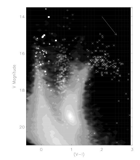
Figure 3: Combined colour magnitude diagram of the 4 target EROS2 SMC fields consisting of 115 000 stars. The grey scale represents number of stars. The HAeBe candidates are indicated by filled squares, the eclipsing binaries by triangles, pulsators by circles, blue variables by asterisks and crosses are both the long period variables and the red irregular variables. The arrow indicates the extinction vector for an extinction of 1 magnitude.

3.2 Selection of blue irregular variable stars

The combined number of 27 blue variable stars and HAeBe candidates listed in Table 2 are objects with average colour of $(V_{\rm E}-R_{\rm E})<0.35$. This colour corresponds to unreddened Galactic main-sequence (MS) stars of type F2 and earlier. In the SMC the colour criterion corresponds to MS star of type A8 and earlier, applying the known foreground extinction towards the SMC of $E(B-V)=0.07$ (Larsen et al. 2000). Among these blue objects a variety of light curves is present (see also Mennickent et al. 2002). We will group these stars on the basis of the observed time scale and amplitude of variations: (A) modulations with distinct periodicity (2 objects); (B) long term ($\mathrel{\hbox to0.0pt{\lower 3.5pt\hbox{$\sim$}\hss}\raise 1.5pt\hbox{$>$}}100$ days) modulations (7 objects); (C) intermediate term ($\rm 3\mathrel{\hbox to0.0pt{\lower 3.5pt\hbox{$\sim$}\hss}\raise 1.5pt\hbox{$<$}}days\mathrel{\hbox to0.0pt{\lower 3.5pt\hbox{$\sim$}\hss}\raise 1.5pt\hbox{$<$}}50$) irregular variations with or without long term modulations with amplitude $\Delta V_{\rm E}>0.2$ (7 objects); (D) intermediate time scale variation with small amplitude $\Delta V_{\rm E}<0.1$ (11 objects).

The expected time scale of brightness changes of the Galactic intermediate mass PMS stars complies with group (C). These seven stars we have termed therefore HAeBe candidates and will be analysed in this paper. The coordinates, magnitude and colour of these 7 HAeBe candidates are given in Table  3. The other 20 blue variables will be discussed in a forthcoming paper.

Table 3: HAeBe candidates discussed in this paper.

Name	EROS2-name	Other design.	RA(2000)	Dec(2000)	$\rm<V>$	$\rm<V-I>$
			(h,m,s)	(${}^{0},^{\prime},^{\prime\prime}$)
ESHC 1	sm00103k-4755	LIN 232	00 53 02.89	-73 17 59.0	15.05	0.06
ESHC 2	sm00103k-2210		00 52 32.73	-73 17 06.9	16.97	0.14
ESHC 3	sm00101l-15299	[MA93] 563	00 52 21.59	-73 13 32.1	16.61	-0.02
ESHC 4	sm00101n-14763		00 53 56.77	-73 10 30.0	14.97	0.09
ESHC 5	sm00101l-3359	[MA93] 535	00 52 06.55	-73 06 29.3	14.02	0.24
ESHC 6	sm00101n-2402	LIN 264	00 54 37.64	-73 04 56.4	15.09	0.04
ESHC 7	sm00103k-6329	[MA93] 619	00 52 52.60	-73 18 33.4	15.27	0.50

Two stars of group (C) were studied photometrically and spectroscopically by Beaulieu et al. (2001). Following their nomenclature we will classify these stars as Eros SMC HAe/Be Candidates, or ESHCs.

We would like to stress that the terminology used, is based on the variability similarities with stars discovered in the LMC (the ELHCs) in Lamers et al. (1999) and De Wit et al. (2002). Some ELHCs have been studied in more detail in LBD. Considering that these are their SMC counterparts, we will use the name ESHC, emphasizing that at present these stars are candidate PMS stars.

4 Description of brightness and colour variations of the ESHCs

The light curves of the ESHCs form the first criterion to identify these objects as such. They are presented in Figs. 4, 5, and 6. Also presented is the corresponding behaviour of the stars in colour-magnitude diagram (CMD). The observations span more than 3 years. On average there are 330 measurements per star. The mean time-interval between observations during an observing season is $\mathrel{\hbox to0.0pt{\lower 3.5pt\hbox{$\sim$}\hss}\raise 1.5pt\hbox{$<$}}2$ days. The error bars are indicated in the CMDs. The EROS2 photometric accuracy for a star of $R_{\rm E}=15^{m}$ is $\sigma(R_{\rm E})\sim 0.02$. The filled circles in the CMDs are the average colours in magnitude bins of 0.02m, provided there are more than 4 measurements in each magnitude bin. The dashed line is a linear fit to these points and the value of the slopes is given in Table 4. These fits have been put to make clear the observed general trend. In the next subsections, we will give a short description of the light curves.

Figure 4: The light curves and corresponding CMDs of ESHC 1 to 4. The time is given as JD-2447892.5 (the time axis runs from 19apr 1996 through 24apr 1999).

Figure 5: The light curves and corresponding CMDs of ESHC 5 and 6. The time is given as JD-2447892.5 (the time axis runs from 19apr 1996 through 24apr 1999).

4.1 The variability of ESHC 1 to 6

In general the light curves do not show any sign of periodicities in their signal, but irregular photometric variations on intermediate time scales ($3\mathrel{\hbox to0.0pt{\lower 3.5pt\hbox{$\sim$}\hss}\raise 1.5pt\hbox{$<$}}\rm days\mathrel{\hbox to0.0pt{\lower 3.5pt\hbox{$\sim$}\hss}\raise 1.5pt\hbox{$<$}}50\,$). Some show long term modulations, e.g. ESHC 1, 2, 3, 4. The maximum difference in brightness over the whole time-span of observations ranges between 0.2 and 0.45 magnitudes in $V_{E}$ (see Table 4). Some ESHCs show features in their light curve which maybe best termed by outbursts: an increase in brightness is followed by a slow relaxation to the original flux level. In particular, the observations of ESHC 4 indicate (possibly) four outbursts. Two outbursts (at days 2485 and 2935) seem to be well covered by the observations. They last for 90 and 45 days respectively. In both cases the decrease towards the initial flux level takes twice as long as the rising part. During the rise, the colour of the object becomes increasingly redder (see Sect. 8 for a discussion of the possible causes for the observed brightness and colour behaviour). The same holds for a large outburst at day 2503 of ESHC 6. The brightness increase of ESHC 3 at day 2921 seems to be symmetric. The amplitude of the observed outbursts varies between $0.1^{m}$ and $0.2^{m}$. The range in time-span of the observed outbursts in the different ESHCs varies between 45 and 90 days. The outbursts with the largest brightness increases seem to persist the longest.

In contrast, star ESHC 5 seems to preferentially decrease in brightness from the average flux level. This star displays variations on a somewhat shorter time scale than the other ESHCs. The colour of the object hardly changed during the observations, while its brightness varied with $\Delta V_{\rm E}=0.25^{m}$. Although to a lesser extent, ESHC 6 might display decreases in brightness. This is particularly observable from day 2800 onward.

During its first season of observation star ESHC 1 shows quasi-regular brightness variations on a $\rm\sim\,30day$ time scale, superposed on a longer time scale increase. In the second and third season it is mainly at brightness minimum. Star ESHC 2 exhibits more pronounced long term modulation (see also Beaulieu et al. 2001).

Examining the CMDs, one notices that for ESHC 1, 2, 3, 4 and 6 the variations are anti-correlated with the brightness of the star, i.e. it is ‘redder-when-brighter’. ESHC 5 is an exception. Quantitatively, the slope of $d(V_{\rm E}-R_{\rm E})/dV_{\rm E}$ in a CMD should then have a negative value. We have measured these slopes using a linear least-squares fit to the average colour in a magnitude bin of 0.02m containing at least 4 measurements (filled symbols in the CMDs). The values of this slope for ESHC 1 to 6 are tabulated in Table 4. Only the slope of ESHC 5 is compatible with grey variation.

4.2 The variability of ESHC 7

ESHC 7 (Fig. 6) has the largest amplitude of brightness variations compared to the other 6 ESHCs. The variations exhibit the same trend, viz. a slow decrease followed by a sharp rise. Peculiarly, the deeper the brightness minimum, the faster the subsequent increase is (for the deepest minimum $\rm-0.018^{m}\,day^{-1}$ for the shallowest $\rm-0.008^{m}\,day^{-1}$). Part of the CMD of ESHC 7 the faint part is anti-correlated with its brightness (i.e. ‘bluer-when-fainter’), similar to ESHC 1, 2, 3, 4 and 6. However this is only the case when the star is in a brightness minimum. The colour behaviour is different when the star is at brightness maximum ($V_{\rm E}<15.2$). Then the colour variations show the opposite (i.e. ‘redder-when-fainter’).

This behaviour is made more clear in the CMD. The dashed line connects the consecutive measurements between day 2380 and 2480. During this phase the star faded to its deepest observed brightness minimum. Notice that during the initial fading phase the star follows a ‘redder-when-fainter’ branch. Remarkably the slope of the measurements follow the expected slope arising from extinction by normal IS dust (with $\rm R_{V}=3.3$). When the star has decreased its brightness to $V_{\rm E}\sim 15.20$, a colour reversal occurs and the star follows a ‘bluer-when-fainter’ branch.

Figure 6: The light curve and CMD of ESHC 7. The star first becomes redder when it fades according to IS extinction by normal dust (indicated by the arrow for an $E(B-V)=0.10$). Then it reverses its trend and becomes ‘bluer-when-fainter’. The dashed and full lines indicate consecutive measurements. For a description of the brightness-colour cycle see text.

This reversal in colour behaviour (from redder to bluer) during the fading of the star, is a well known and well studied behaviour of the UX Orionis subgroup (UXOrs) of PMS stars. It is understood in terms of obscuration by circumstellar dust clouds, which causes the star to become redder when it fades initially. The growing relative contribution of blue scattered radiation to the total observed radiation due to the (unobscured) proto-planetary disk halts the reddening colour trend, and makes it again bluer (Zaitseva 1987, Voshchinnikov et al. 1988, Eaton & Herbst 1995, Grady et al. 2000, Natta et al. 2000 and references therein).

However, contrary to what has been observed among UXOrs, during its rise out of the first observed deep minimum, ESHC 7 follows a third and different branch. The star brightens at day 2463, but the colour does not change. The corresponding measurements are connected by the full line in Fig. 6. It follows a track almost straight up, nearly reaching its initial brightness. This cycle is partly repeated during the second minimum at day 2535. The time the star spends in this minimum is shorter than during the first minimum. After this second brightness minimum, the observed flux increases at about constant colour, but in this case it does not reach its maximum value. Consequently the star will join the colours corresponding to the fading track, close to the position of the colour reversal. In Fig. 6 these are the measurements between $V_{\rm E}\sim 15.35$ and $V_{\rm E}\sim 15.20$ and colour $V_{\rm E}-R_{\rm E}\sim 0.33$ and $V_{\rm E}-R_{\rm E}\sim 0.35$ (see also Fig. 15).

Summarizing, the brightness-colour cycle for ESHC 7 consists of three parts. Starting at brightness maximum: (1) a ‘redder-when-fainter’ portion when $V_{\rm E}\mathrel{\hbox to0.0pt{\lower 3.5pt\hbox{$\sim$}\hss}\raise 1.5pt\hbox{$<$}}15.2$, (2) a ‘bluer-when-fainter’ portion when $V_{\rm E}\mathrel{\hbox to0.0pt{\lower 3.5pt\hbox{$\sim$}\hss}\raise 1.5pt\hbox{$>$}}15.2$ and (3) a grey portion, to return to the initial brightness. We will discuss this behaviour in Sect. 8.1.4.

Table 4: The photometric measurements of the ESHCs.

	EROS2				ESO				2MASS
Name	$<V_{\rm E}>$	$<V_{\rm E}-R_{\rm E}>$	$\Delta V_{\rm E}$	$d(V_{\rm E}-R_{\rm E})/dV_{\rm E}$	V	B-V	V-R	V-I	J	J-H	H-K
(1)	(2)	(3)	(4)	(5)	(6)	(7)	(8)	(9)	(10)	(11)	(12)
ESHC 1	15.04	0.03	0.25	$-0.24\pm 0.02$	15.06	0.00	0.00	0.04	15.05	0.09	0.13
ESHC 2	16.95	0.08	0.40	$-0.33\pm 0.03$	17.00	-0.06	-0.01	0.03	-	-	-
ESHC 3	16.61	-0.01	0.20	$-0.33\pm 0.07$	-	-	-	-	-	-	-
ESHC 4	14.99	0.07	0.20	$-0.16\pm 0.04$	-	-	-	-	15.02	0.06	0.13
ESHC 5	13.98	0.19	0.25	$0.04\pm 0.07$	-	-	-	-	13.48	0.12	0.09
ESHC 6	15.11	0.03	0.30	$-0.08\pm 0.03$	-	-	-	-	15.02	0.07	0.34
ESHC 7	15.17	0.34	0.45	–	15.12	0.31	0.25	0.57	14.36	0.16	0.25

5 H$\alpha$ emission and cross identification with SIMBAD

Herbig Ae/Be stars are (partially) defined as having emission line spectra. Therefore we systematically searched for cross identifications of the target stars with archive catalogues using the SIMBAD database operated at Strasbourg, France. Some ESHCs are reported as emission line stars in different SMC objective prism surveys (Lindsay 1961, Meyssonnier & Azzopardi 1993 (MA)). MA classifies the observed H$\alpha$ profile and the observed continuum around the line. The H$\alpha$ emission of ESHC 5 is classified as “moderate strength and peaked”. The H$\alpha$ line of ESHC 7 is classified as “moderate strength and appreciably widened”. For ESHC 3 the detection of H$\alpha$ emission is given as “doubtful”.

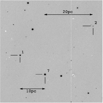
Figure 7: A subtracted $\rm H\alpha-H\alpha_{cont}$ image. The panel shows ESHC 1, 2 and 7. Note that the stars are located within 35pc of each other.

The existence of H$\alpha$ emission is verified for 3 stars with the narrow band imaging we obtained in 1998 (see Sect. 2.2). We have built a subtracted image of ($\rm H\alpha-H\alpha_{cont}$) using ISIS, the image subtraction package with non constant kernel (Alard 2000). The resulting subtracted image is at 30% of the photon noise. We show the resulting image in Fig. 7. All the objects in the image are H$\alpha$ emitters, the brightest of which have been published before by Lindsay (1962) and Meyssonnier & Azzopardi (1993). The nature of these objects remains to be investigated, but they can be such objects as PMS stars, PNe, H ii regions, classical Be stars, symbiotic systems, massive stars with winds. We have indicated stars ESHC 1, 2, 7. These stars are clearly visible as H$\alpha$ emitters and are located within 35pc of each other.

6 The location of ESHCs in the SMC and their correlation with Far-IR emission

Regions with far IR (FIR) emission can be used as a tracer of massive star formation. This was shown by Mead et al. (1990). In Fig. 8 we present a $\rm 60\mu m$ image taken with IRAS. It shows the positions of the ESHCs (filled dots) in the bar of the SMC. The contours represent stellar densities, which were determined from a Digital Sky Survey image. Within the central contour (thickest line) the highest stellar density is present. Note that the FIR emission does not follow the distribution of stars. The maximum level of FIR emission (in MJy/sr) is visible at the far west in the image. Fig. 8 shows an enhancement of FIR emission in the central part. There are 3 ESHCs (1, 2, 7) grouped on the south edge of the enhancement and ESHC 4 is on the east edge. ESHC 3 is located within the FIR emission region. The other 2 stars are located outside the region. Its emission level is at 25% of the maximum of 65 MJy/sr. The lowest level of the IRAS image is at 5% of the maximum. The four rectangles represent the EROS2 fields from Table 1.

Fig. 8 shows that both the HAeBe candidates and the blue variables are generally (but not specifically) associated with the $\rm 60\mu m$ excess emission, i.e. a region which is likely to have a young stellar population. The lack of any detection of blue variables in the lower right rectangle (which is EROS2 field sm00103m) is noticeable, the more so, as the numbers of LPVs and pulsating stars in this particular field are comparable to the other three EROS2 fields. Field sm00103m is the furthest from the central $\rm 60\mu m$ emission region compared to the other three examined EROS2 fields.

A correlation between FIR emission and location of HAeBe candidates in the LMC was found by De Wit et al. (2002). These stars were shown to be associated with a $\rm 60\mu m$ excess emission region in the bar of the LMC.

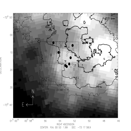
Figure 8: An IRAS image of the SMC at $\rm 60\mu m$. The FIR emission is presented on a linear grey scale and is in units of MJy/sr. Indicated are the ESHCs (filled dotes), the blue variables (open circles). Overlaid are the fields corresponding to the EROS2 CCDs (large squares) and isophots of the SMC. Increasing thickness of the isophots means increasing stellar densities. Notice that 5 ESHCs are associated with a slight enhancement of the $\rm 60\mu m$ emission.

7 Deriving stellar parameters from SED fitting

In Sect. 2.2 we described $BVRI$ and H$\alpha$H$\alpha_{cont}$ photometry for three fields in the SMC. These observations were not specifically done on the fields in which the ESHCs are located. However three ESHCs were within the field of view of these observations.

In order to analyse the SED from visual to NIR, we performed a cross identification with the 2MASS (2 Micron All Sky Survey) second incremental data release (via http://irsa.ipac.caltech.edu). The limiting magnitudes of 2MASS data for the detection of point sources with an $\rm S/N\mathrel{\hbox to0.0pt{\lower 3.5pt\hbox{$\sim$}\hss}\raise 1.5pt\hbox{$>$}}10$ are $J\leq 15.8^{m}$, $H\leq 15.1^{m}$ and $K_{s}\leq 14.3^{m}$. We searched for sources within 10” of the target position. We checked the positions of the resulting sources with the astrometrically calibrated optical images described in Sect. 2.2. Available $\rm JHK_{s}$ measurements were found for the 5 brightest ESHCs. Thus, we have coverage of the SED from the visual to the NIR for 3 ESHCs c.f. 1, 2 and 7. All photometric measurements are listed in Table 4.

We compared the $(B-V)$, $(V-I)$ and $(V-R)$ colours of the ESHCs with model predictions to derive the effective temperature and/or the CS extinction. We chose not to use the $\rm JHK_{s}$ measurements in the fitting procedures. We used Kurucz models calculated for the appropriate metallicity for the SMC, $\rm[Fe/H]=-1.0$. A minimal foreground extinction of 0.07 in $E(B-V)$ was applied, using the extinction law with $R_{v}=3.3$ from Cardelli, Clayton & Mathis (1989). In case of ESHC 1 and 2 the stellar parameters have been derived from spectroscopy by Beaulieu et al. (2001), viz. ESHC 1: $\rm log(T_{\rm eff})=4.20$, $\rm log(L/L_{\odot})=4.23$, ESHC 2: $\rm log(T_{\rm eff})=4.34$, $\rm log(L/L_{\odot})=3.84$. We used the constraints from their intrinsic colours to derive the CS extinction by fitting for a minimum $\chi^{2}$. For ESHC 1 the atmosphere models corresponding to their effective temperature did not give a satisfactory fit to the data. We obtained $\chi^{2}=4.9$ for the best fitting model with an $E(B-V)_{cs}=0.06$. For ESHC 2 we obtained a $\chi^{2}=2.4$ for an extinction $E(B-V)_{cs}=0.09$. In case of ESHC 7, we do not have an independent determination of $T_{\rm eff}$ and $\rm log(L/L_{\odot}$). Therefore we fitted for both the temperature and circumstellar extinction. The SED of ESHC 7 fits a model atmosphere of $\rm log(T_{\rm eff})=3.94^{+0.06}_{-0.06}$ with a $\chi^{2}=1.7$. The corresponding CS extinction is $E(B-V)_{cs}=0.19\pm 0.07$. The derived temperature of ESHC 7 indicates an A-type star. We calculated its absolute visual magnitude, i.e. $M_{V}=-4.74^{+0.20}_{-0.20}$ with the SMC distance modulus of 18.94 (Laney & Stobie 1994).

We adopt the bolometric correction of -0.184 which follows from the best fitting Kurucz model. This results in a $\rm log(L/L_{\odot})=3.87^{+0.14}_{-0.18}$. The uncertainty in the derived luminosity of ESHC 7 is estimated from the uncertainty in the effective temperature (bolometric correction) and extinction from the model fit, allowing all models which are within the internal error ($\sum_{i=1}^{N}1/\sigma_{i}^{2}$) of the photometric measurements.

With respect to the EROS coverage of the light curves of the ESHCs, the optical photometric measurements were obtained at day 2929 of Figs. 4, 5, and 6, whereas 2MASS observed the ESHCs on 9sep 1998, corresponding to JD 2451034.5 or day 3142 in the same figures. Hence we see that for ESHC 1, 2 and 7 the optical and NIR photometric data for each object were taken during nearly equal brightness states. Obviously, there is a dependence of the determined parameters on the variability. For ESHC 1 and 2, the derived extinction will be larger when the stars are in a brighter state. For ESHC 7, the photometric measurement correspond to a high brightness state, in which the colour of the star is most blue. The derived stellar parameters for ESHC 7 may change when fitting broad-band UBVI measurements taken at a different epoch, depending on the physical mechanism causing the variability.

The SEDs from B-filter to $\rm K_{s}$-filter of ESHC 1, 2 and 7, with the atmosphere models corresponding to the temperatures derived from spectroscopy (ESHC 1 and 2) and the SED fit (ESHC 7) are presented in Figs. 9 to 11. The measurements of the stars are corrected for extinction using the found values of $E(B-V)$, as described. We conclude from these figures that ESHC 1 and 7 are brighter in $\rm JHK_{s}$ filters than expected from stellar atmosphere models.

We will discuss the NIR excess in Sect 8.2.

Figure 9: Spectral energy distribution for ESHC 1. The NIR points are 2MASS data. The full lines are Kurucz atmosphere models for a metallicity $\rm[Fe/H]=-1$.

Figure 10: Spectral energy distribution for ESHC 2. Upper limits for a S/N=10 from 2MASS are indicated.

Figure 11: Spectral energy distribution for ESHC 7. The NIR points are 2MASS data.

8 Discussion of ESHC properties

We have discussed 7 blue irregular variables in the SMC. The purpose was to identify PMS stars at a lower than solar metallicity. Some of these stars (see Sect. 6) are located near or on the edge of a region where an increase in $60\mu$ emission has been detected by IRAS. FIR emission has been shown to be a tracer of massive star formation (Mead et al. 1990). We have labeled them HAeBe candidates primarily on the basis of their brightness variations, as an initial working definition. A number of criteria exist to determine whether a star is a genuine member of the PMS HAeBe group. Some criteria are degenerate with the characteristics of classical Be stars, viz. H$\alpha$ emission, irregular variability and near IR excess. In the next subsections we will discuss and compare these properties of ESHCs with the known properties of HAeBe stars and classical Be stars.

8.1 Causes of ESHC brightness variability

Post-Main Sequence classical Be stars (B type stars of luminosity class III to V, which show or have shown in the past the Balmer series in emission) tend to be variable on several time scales and with a range of amplitudes. A summary of light curves of Be stars over a 20 year period have been published by Pavlovski et al. (1997). Random brightness outbursts among early-type Be stars have been measured by Hipparcos and discussed by Hubert & Floquet (1998). These occur on time scales between 20 to 500 days with $\Delta Hp\mathrel{\hbox to0.0pt{\lower 3.5pt\hbox{$\sim$}\hss}\raise 1.5pt\hbox{$<$}}0.3^{m}$. The time scale of the outbursts depends on the amplitude. On short-term time scales ($\rm\mathrel{\hbox to0.0pt{\lower 3.5pt\hbox{$\sim$}\hss}\raise 1.5pt\hbox{$<$}}days$) Be stars vary predominantly periodically with moderate amplitudes, $\Delta V<0.1^{m}$ (Feinstein & Marraco 1979). These short-term time scales could either be caused by non-radial pulsations or by rotation modulations (see Baade & Balona 1994). The large amplitude, long-term outbursts can be interpreted as variable emission from the hot gaseous circumstellar environment (Waters et al. 1987, Dachs et al. 1988). In this case, the additional red flux from the disk will cause the brightness to increase, and at the same time the observed SED to become flatter. The combined flux of star and disk will increase but will have a redder colour (e.g. Dachs 1982).

Pre-main sequence Herbig Ae/Be stars exhibit a large range of types in photometric and spectroscopic variability. Generally, brightness levels of HAeBe stars seem to be quasi-periodic, on time scales of $\rm\sim year$ with $\Delta V\sim 0.1^{m}$ (Herbst & Shevchenko 1999). Superposed are random brightness decreases, which can have large amplitude $\Delta V\mathrel{\hbox to0.0pt{\lower 3.5pt\hbox{$\sim$}\hss}\raise 1.5pt\hbox{$>$}}1^{m}$. The early type Herbig Be stars ($\rm<B8$) however, tend to be low amplitude irregular variables with $\Delta V<0.2^{m}$ (Finkenzeller & Mundt 1984, Van den Ancker et al. 1998, Herbst & Shevchenko 1999). Obscuration of the central stars by a varying amount of circumstellar dust is the most quoted mechanism to explain these variations (see Wenzel 1969, Thé 1994). Although unsteady mass accretion as the dominant cause has also been proposed by Herbst & Shevchenko (1999).

We will explore the brightness and colour variations exhibited by the ESHC stars in terms of the two physical processes quoted for Pre-MS and Post-MS Be star variability: (1) bound-free and free-free (bf-ff) gas emission, (2) variable dust obscuration. Both mechanisms are capable of causing a ‘redder-when-brighter’ behaviour. In case (1) this is caused be an increase in the total flux, while in case (2) it is required that an extensive blue scattering source is present, which will dominate when the total stellar flux decreases (and thus in fact ‘bluer-when-fainter’).

In the next subsection we will first determine the sensitivity of variable H$\alpha$ emission on the EROS2 broad filters. This is important as both HAeBe stars (e.g. Catala 1999, Pogodin et al. 2000) as well as classical Be stars (inherent to their definition) are known to exhibit variations in the equivalent width (EW) of H$\alpha$. For Be stars an H$\alpha$  variability of 50A seems to be maximum (see Dachs 1988, Banerjee et al. 2000). Whereas an HAeBe star like HD 200775 can increase its EW(H$\alpha)$ from 55Å to 105Å (Pogodin et al. 2000).

8.1.1 The influence of H$\alpha$

A variable EW of the H$\alpha$ line influences $V_{\rm E}$ and $R_{\rm E}$ passbands differently and hence the colour will change as a function of the H$\alpha$ EW. We will determine the qualitative contribution of H$\alpha$ to the EROS2 photometry. An increasing amount of flux was added to the H$\alpha$ line of a synthetic B type spectrum of $T_{\rm eff}=23\,000{\rm K}$. At each increase we folded the $V_{\rm E}$ and $R_{\rm E}$ response curves with the spectrum in order to calculate the subsequent altered magnitudes and colour. In Fig. 12 we illustrate the dependence of $V_{\rm E}$ on H$\alpha$ EW and the subsequent change in $V_{\rm E}-R_{\rm E}$.

Figure 12: The correlation between colour as function of $V_{\rm E}$ magnitude. The corresponding $\rm H\alpha$ equivalent widths (in Å) are indicated.

We note that the influence of variable H$\alpha$ emission on the magnitudes is small. Its influence on the total flux in the $V_{\rm E}$ filter is 4.4% at an EW level of 180Å, while it is 7.0% on $R_{\rm E}$. This leads to a minor increase of $\sim 0.05^{m}$ and $\sim 0.08^{m}$ in magnitude, respectively. The observed maximum amplitude of variation of the ESHCs, listed in Table 4, is much larger. However their small amplitude variations are of the same value as predicted for strong H$\alpha$ variation.

We can calculate the necessary EW variations in the case of ESHC 1 and 2, if all the observed variations were caused by H$\alpha$ variations. Beaulieu et al. (2001) measured an H$\alpha$ EW of $\rm 2.6\AA$ and $\rm 16.5\AA$, respectively. ESHC 1 has an amplitude of variation of $0.33^{m}$ in $V_{\rm E}$. Then the EW should increase to $\rm 1300\,\AA$ to cause $\Delta V_{\rm E}=0.33^{m}$, hence an increase of almost 500 times. For ESHC 2 the required H$\alpha$ variation is less, a factor 100.

Because the influence on $R_{\rm E}$ is larger than on $V_{\rm E}$, a change in the EW of the H$\alpha$ line will cause the star to become bluer when it fades. The subsequent slope of $d(V_{\rm E}-R_{\rm E})/dR_{\rm E}$ in Fig. 12 equals $-0.58$. None of the measured slopes of the ESHCs have this value. Therefore we conclude that the photometric variations are not solely due to a variation of the H$\alpha$ equivalent width.

8.1.2 The influence of variable bound-free and free-free emission

In this section we present a comparison of the observed brightness and colour variations of the program stars with an outflowing disk surrounding a classical Be star. The method was presented by Lamers & Waters (1984) for spherically symmetric stellar winds and adapted by Waters (1986) for a non-spherically symmetric configuration to explain the observed infrared (IR) excess emission of Be stars in terms of mass loss. It assumes bf-ff radiation from an isothermal, equatorial, gaseous outflowing disk, which is viewed at most pole-on (henceforth to be called ff-disk). In a subsequent paper Waters et al. (1987) showed that the observed ‘redder-when-brighter’ behaviour in a (B-V)-V diagram of the Be star $κ$ CMa (Dachs et al. 1986) can be explained by an increase of the ff-bf radiation of the equatorial ff-disk. When the number density of charged particles (parameterized by the emission measure $\rm EM=\int n_{\rm E}^{2}dV$) in the ff-disk increases, the total flux radiated by the ff-disk will increase more in the lower energy part of the spectrum than in the higher energy part.

Lamers & Waters (1984) derived an analytical expression for the monochromatic excess flux ratio ($\Delta F_{\nu}^{tot}/F^{*}_{\nu}$) as a function of the temperature of the outflowing material, the stellar radius, and the EM. We will use the expression as it was presented in Eq. 15 in Waters (1986). This equation is valid in the optically thin case. It can be applied if the stellar parameters are known, viz. for ESHC 1, 2 and 7. We can calculate the increase in flux in the $V_{\rm E}$ and $R_{\rm E}$ filters due to an increase of bf-ff emission and compare this to the observed photometric measurements of ESHC 1 and 2. For the calculation of the monochromatic excess flux we first determined the effective wavelengths of the EROS2 filters as a function of spectral type. We used blackbody spectra with the effective temperatures of ESHC 1 an 2. For a B4 star (ESHC 1) $\lambda_{\rm eff}$ is $\rm 5880\AA$ and $\rm 7380\AA$, for $V_{\rm E}$ and $R_{\rm E}$ respectively. The difference in $\lambda_{\rm eff}$ for a B2 star (ESHC 2) is marginal.

In Figs. 13 and 14 we show the CMDs of ESHC 1 and 2. The solid lines with tick marks represents the optically thin ff-disk model. Following Waters (1987), we assumed that the temperature of the ff-disk is 0.8 times the effective temperature of the star. We assumed that at brightness minimum the EM of the ff-disk is negligible and we set its value to 0. The figures show that the observed relationship for ESHC 1 between visual brightness and colour is compatible with an outflowing isothermal ff-disk, which increases its EM to $\rm 1.6x10^{61}\,cm^{-3}$, although the scatter is large. The maximum EM for ESHC 2 is less, $\rm 7x10^{60}\,cm^{-3}$.

The model translates into an excess emission due to the contribution of the ff-disk. Therefore, the magnitude and colour of the B star itself is assumed to be observed when the stars are at their faintest. These colours should correspond to the intrinsic colours inferred from the spectral types derived by Beaulieu et al. (2001). From Figs. 13 and 14 we read that ESHC 1 at brightness minimum has $V_{\rm E}\sim 15.15^{m}$ and $V_{\rm E}-R_{\rm E}\sim-0.03$, while ESHC 2 has $V_{\rm E}\sim 17.1^{m}$ and $V_{\rm E}-R_{\rm E}\sim 0.00$.

We converted the spectral types to the $V_{\rm E}-R_{\rm E}$ colour. We adopted the $T_{\rm eff}$-$(V-I)_{0}$ conversion for SMC metallicity from Kurucz models. We applied the transformation equations from Sect. 2.1.1 and corrected for the IS extinction towards the SMC. Then we derive a $V_{\rm E}-R_{\rm E}=-0.04$ for ESHC 1 and $V_{\rm E}-R_{\rm E}=-0.10$ for ESHC 2.

There is a very good agreement between the derived spectroscopic colour of ESHC 1 and its observed colour at its faintest state. The assumption of a ff-disk causing the emission excess holds for ESHC 1.

The derived spectroscopic colour and the observed colour in the faint state do not agree for ESHC 2. The spectroscopic colour is bluer. The discrepancy can be resolved in two ways. Either (1) at its faintest phase the EM is non-zero, i.e. substantial emission from the ff-disk is still present, causing the colour to be redder than the colour derived from spectroscopy or (2) there is an additional CS extinction.

Case (1) implies that the underlying star is intrinsically much fainter than the minimal observed brightness of the EROS2 light curve. We calculated a ff-disk model using the spectroscopic colour of -0.10. It is represented by the dashed-dotted line in Fig. 14. In its faintest observed state, a ff-disk is present. An EM of zero (no ff-disk) is found at a $V_{\rm E}$ magnitude of 17.6. This model does not agree with the observed photometric measurements. The full line in Fig. 14 represent a star+ff-disk system which is subject to a CS extinction of $E(B-V)_{CS}=0.12$. In this model it is assumed that no ff-disk is present in the faintest observed state. This model is compatible with the EROS2 observations. The resulting dereddened magnitude of the underlying B star in this case is $V_{\rm E}=16.8^{m}$.

We conclude that in the case of ESHC 1 the ‘bluer-when-fainter’ behaviour can fairly well be explained by an increase in the EM of the ff-disk. During some epochs, the ff-disk contribution is marginal and the intrinsic colours of the star is observed. These colours correspond to the colours derived from the spectral type, corrected for interstellar extinction. This is compatible with the notion of the ’Be-phenomenon’, i.e. stars temporarily go through a Be phase. However the required maximum EM is high. Galactic stars of the same spectral type have a typical EM which is an order of magnitude less (Waters et al. 1987). Their detailed calculations give a maximum EM of $7.9\rm{x}10^{59}\,cm^{-3}$ for a B4e type star, whereas a value of about $1.2\rm{x}10^{61}\,cm^{-3}$ is required to explain the excess emission observed in ESHC 1.

The case of ESHC 2 is more complicated. A CS extinction of $E(B-V)_{CS}\sim 0.12$ is needed in order to let the ff-disk model fit. The same extinction value was found in the best fit of the SED (Sect. 7). The extinction should originate in a region outside the ff-disk. Furthermore, at the blue end of the CMD, the $V_{\rm E}$ magnitude of ESHC 2 seems to be constant while the colour gets bluer. This cannot be explained by the ff-disk model. Comparing the derived EM for ESHC 2 with Galactic Be stars, we find that the maximum EM is higher than Be stars of similar spectral type. Waters et al. (1987) derive a maximum EM (model inferred, based on IRAS measurements) of $2.5\rm{x}10^{60}\,cm^{-3}$ for a B2e type star, whereas a value of about $6\rm{x}10^{60}\,cm^{-3}$ is required to explain the excess emission observed in ESHC 2. The derived large EM could just be a selection bias due to our variability criterion. We selected Be stars displaying the largest variability amplitude.

The exhibited brightness colour relation of ESHC 7 cannot be explained by a ff-disk model only. The increase in flux originating in the ff-disk will always make the star ‘redder-when-brighter’, whereas we observe ‘redder-when-fainter’ and peculiar ‘grey’ phases. Therefore we conclude that it is unlikely that the variability of ESHC 7 is caused by variable ff-disk emission. We did not specifically fit this star with the Be ff-disk model.

For the objects for which we did not fit with the ff-disk model (i.e. ESHC 3, 4, 5 and 6), the analysis of the light curves presented in Sect. 4, shows that three of them (ESHC 3, 4, 6) exhibit bursts of emission. This phenomenon is preferentially observed among the early type classical Be stars. During the outbursts the colour of the Be star gets redder with a colour gradient of $\Delta(B-V)/\Delta V\sim-0.1$ to $-0.3$ (Dachs 1982). The measured $d(V_{\rm E}-R_{\rm E})/dV_{\rm E}$ is tabulated in Table 4. ESHC 3 and 4 have a gradient which is similar to the gradient of classical Be stars. The gradient of ESHC 6 is smaller, but still compatible with a Be ff-disk. The brightest star in the sample (ESHC 5) displays a different light curve than stars 3, 4 and 6, moreover its colour gradient is compatible with grey extinction. Therefore the photometric properties of this star will not be accurately described by a ff-disk.

Figure 13: Colour-Magnitude diagram of ESHC 1. The solid line represents the optically thin ff-disk model (Sect. 8.1.2). The tick marks on the model fit indicates the increase in EM (to upper right corner) in steps of $\rm 0.2\,x\,10^{60}\,cm^{-3}$ to a maximum of $\rm 1.4\,x\,10^{61}\,cm^{-3}$. The dashed lines represent obscuration model fits with an CS $R_{V}$ of 3.3 (right one), the dot-dashed line has a CS $R_{V}$ of 5.0 (left one). Average error bar is indicated in the lower right corner and a reddening vector (corresponding to value of $E(B-V)=0.1$) in the upper left corner.

Figure 14: Same as Fig. 13, but for ESHC 2. The tick marks on the ff-disk model fit (solid line) indicates the increase in EM in steps of $\rm 1\,x\,10^{60}\,cm^{-3}$ to a maximum of $\rm 5\,x\,10^{60}\,cm^{-3}$ This model fits if a CS extinction of $E(B-V)=0.12$ is applied. The extinction vector is indicated by the arrow and corresponds to a value of $E(B-V)=0.1$. The dotted line is an ff-disk model assuming that the total colour excess with respect to the intrinsic colour is only due to ff-disk emission. The dashed lines represent obscuration models for $R_{V}$ of 5.0 (left one) and 3.0. The colour of the applied scattering nebula is 0.04. An IS extinction was applied of $E(B-V)_{IS}=0.05$. A reddening vector corresponding to $E(B-V)=0.1$ is given. The figure is truncated on the $V_{\rm E}$-axis.

8.1.3 The influence of variable dust obscuration

Obscuration by a variable optical depth of an inhomogeneous circumstellar dust distribution has been successful in explaining the observed photometric and polarimetric behaviour of UXOrs (recently reviewed by Natta et al. 2000). The stars in question are mostly Herbig Ae or T Tauri stars with large $\Delta V>2^{m}$ amplitude variations. These occur randomly in time by screening of the stellar flux by circumstellar dust clouds. During these deep brightness minima they show the ‘bluer-when-fainter’ effect (e.g. Gahm et al. 1993, Grinin et al. 1994, Eaton & Herbst 1995). The blue flux is ascribed to scattering by small dust particles of the unobscured part of the dusty CS-disk/envelope of the HAeBe (Grinin 1988, Natta & Whitney 2000).

Lamers et al. (1999) and De Wit et al. (2002) analysed the observed ‘bluer-when-fainter’ behaviour of Large Magellanic Cloud HAeBe candidates (ELHCs). In contrast to Galactic UXOrs the colour of about $50\%$ of these stars always becomes bluer when the star dims. They argue that this is a resolution effect. An unresolved blue scattering nebula is present around the ELHCs (which was one of the original criteria of Herbig 1960). The nebula is much larger than the star. In this case when the central star fades, the relative contribution to the total flux of the scattering nebula will increase and the colour of the star+nebula system will become bluer. This is strongly suggested by the derived negative extinction for some ELHCs, as determined by Lamers et al. (1999). They compared the intrinsic colours determined from the spectral type with the observed colours at maximum brightness. The observed colours were bluer than the intrinsic colours. This produces a negative extinction correction, indicating the presence of an additional source of blue flux.

It is important to note that there exists a difference between the scattering regions as interpreted for galactic HAeBes and ELHCs. For HAeBes the scattering region is in the direct vicinity of the star-disk system (i.e. a dusty disk atmosphere). In the case of ELHCs the scattering region is assumed to be located relatively far away. The blue flux is interpreted coming from an extended scattering circumstellar cocoon comparable to the one existing around the Galactic HAeBe star V380 Ori.

Following the arguments of Lamers et al. (1999) and De Wit et al. (2002), we can infer blue scattering nebulae surrounding the ESHCs from the observed ‘bluer-when-fainter’ behaviour. These nebulae are not resolved due to the resolution limitations of our ground based observations, where 1 arcsecond corresponds to 0.3 pc in the SMC.

A full description of a star-nebula system using broad band photometry is tentative. Using the analytical model described in De Wit et al. (2002) we can calculate zeroth order estimates of the brightness and colour of the scattering nebula. In the following the term extinction covers all processes which contribute to both true absorption and scattering. The model consists of three components (1) the star, (2) the occulting dust cloud and (3) the scattering nebula which is assumed to be spherically symmetric. The dust cloud is approximately of stellar size, and varies only in optical depth. The scattering nebula is much larger than the obscuring cloud. During an observed brightness decrease, only the star is obscured by the dust cloud. There is no contribution to the flux by the occulting cloud itself. The scattering nebula does contribute to the absorption of the stellar flux in the line of sight, because the nebula is assumed to be circumstellar. In this way, the total extinction of the stellar flux is then determined by the interstellar extinction, the nebular extinction and the extinction due to the occulting dust cloud. Then, the difference with the observed flux is due to the constant (scattered) flux contribution of the nebula. The basic principle is that both the amount of scattered nebular flux and the amount of extincted stellar flux by the obscuring dust cloud will determine the observed amplitude of variation.

As input observables for our model we use (1) the intrinsic colours determined from the spectral type, (2) the amplitude of variation, and (3) the magnitudes at maximum brightness. We assume that at minimum brightness the obscuring cloud is optically thick, i.e. completely blocking the stellar radiation. In this way, we obtain the monochromatic scattering optical depth of the inferred nebula, using the observed amplitude of variation. This is expressed in Eq. (5) of De Wit et al. (2002). We assume that at maximum brightness the stellar radiation is attenuated only by nebular absorption and not by the obscuring dust cloud. In this way, we obtain the monochromatic absorption optical depth of the inferred nebula, using the spectral type. Now we can determine the (constant) nebular flux in $V_{\rm E}$ and $R_{\rm E}$. Using the optical depth of the obscuring dust cloud as a free parameter, we can calculate the resulting colour variation as a function of brightness of the star+nebula system.

Dust surrounding young stars can be of an anomalous nature. This affects the selective to total extinction. Therefore in our calculation we treated interstellar (IS) grains and the circumstellar grain composition (both obscuring dust cloud and the scattering nebula) separately. For IS dust we used $R_{V}=3.3$, while we fitted the CS $R_{V}$ as a free parameter. Moreover, we tried to find the best solution by varying the amount of IS extinction. This is of importance because the applied amount of IS extinction affects the determination of the nebular absorption optical depth, and hence the final nebular flux.

As illustration we present the case of ESHC 1 and 2 in Figs. 13 and 14 to facilitate comparison with the Be star ff-disk model. In both figures we plotted models with different $R_{V}$ for the CS dust, namely 5 and 3.3. The model fits are indicated by the dashed lines. The optical depth of the obscuration cloud ranges from 0.2-7.5 for ESHC 1 and from 0.3-4.9 for ESHC 2. The characteristics of the nebula and the model parameters are given in Table 5

Table 5: Model parameters and nebula characteristics calculated with the obscuration model. Quoted values are for $R_{V}=3.3$ (see text).

Name	$V_{\rm E}^{neb}$	$(V_{\rm E}-R_{\rm E})^{neb}$	$E(B-V)_{IS}$	$E(B-V)_{CS}$	$\tau_{scat}^{Ve}$	$\tau_{abs}^{Ve}$	$\tau_{scat}^{Re}$	$\tau_{abs}^{Re}$
ESHC 1	15.23	0.031	0.04	0.2-7.5	1.45	0.40	1.03	0.24
ESHC 2	17.19	0.042	0.05	0.3-4.9	1.03	0.79	0.84	0.47
ESHC 7	15.45	0.32	0.02	0.2-6.5	1.03	0.57	1.06	0.34

The obscuration model is compatible with the observed colour variations. Especially, in the case of ESHC 1, the cluster of points at the brightest phase corresponds to the predicted point at which the blue nebular flux starts dominating the total flux. However the ff-disk model seems a better fit to the measurements of ESHC 1. Calculating a formal $\chi^{2}$ value for the fits, we find that with a value of 18.2 for the ff-disk and a 21.7 for the obscuration model with $\rm R_{v}=5.0$, the ff-disk fits better.

The near constant brightness of ESHC 2 at its faint phase while the colour becomes bluer can be explained with this model as the nebular flux dominating at this epoch (although the scatter of the measurements is large). Such a behaviour can not be explained by the Be ff-disk model. Quantitative comparison using $\chi^{2}$, shows a formally better fit of the obscuration model with $\rm R_{v}=5.0$ then the ff-disk fits, 18.8 against 19.8. We emphasize that the derived values for $\chi^{2}$ in case of ESHC 1 and 2 are statistically insignificant, however we want to show the trends of the colour-magnitude behaviour of the ESHCs in direct comparison to two possible models.

8.1.4 The case of ESHC 7

Figure 15: Dust Obscuration model fit for ESHC 7. The colour of the nebula is 0.32. An IS extinction was applied of $E(B-V)_{IS}=0.02$. The thick line represents a model with an CS $R_{V}$ of 3.3. The dotted line has an $R_{V}$ of 5.0. For clarity purposes we omitted in the figure the measurements corresponding to the grey part of the brightness behaviour of ESHC 7. The reddening vector corresponds to an $E(B-V)=0.1$.

ESHC 7 is most likely an Ae type star, which displays distinct colour variability. As mentioned in Sect. 4.2 this type of variations is most commonly seen in PMS UXOri stars. However there are some differences between the characteristics of UXOr variability and that displayed by ESHC 7. As far as literature goes, a ‘grey’ phase as observed in ESHC 7 has never been observed among UXOrs. The minima of UXOrs are asymmetric, the star recovering more slowly than it fades (Eaton & Herbst 1995). ESHC 7 shows the opposite trend in which the fading part lasts longer. Moreover the time scale and amplitude are somewhat different. UXOrs can experience a deep ($\Delta V>2$) brightness minimum and subsequent recovery to the initial brightness within typically 50 days. In the case of ESHC 7 it takes 100 days to complete its deepest minimum and subsequent recovery to initial brightness of $\Delta V_{\rm E}=0.4$. At least the difference in amplitude can be understood with the assumption of an unresolved and bright scattering nebula.

Dust is likely to play a role in the mechanism which causes the observed variations. This is suggested by the way the star changes its colour during variations at bright phases. At bright phases the colour change complies with what is expected from dust extinction. Therefore we fitted the brightness-colour relation with the dust obscuration model. The result is exemplified in Fig. 15. The ‘grey’ phase has been omitted from the figure. The subsequent model parameters are listed in Table 5. Notice that the scattering efficiency of the nebula is equally efficient in $R_{\rm E}$ as in $V_{\rm E}$. This is consequence of the fact that at brightness minimum it is assumed that the colour is dominated by the scattering nebula. This colour is similar to the observed colour at maximum brightness. Because the colour of the nebula does not change during the obscuration of the central star, the nebula would be observed bluer than the reddened star. A similar conclusion can be drawn from the observed variation of UXOri in the V-(V-I) plane (Grinin et al. 1994). The star+nebula model gives a reasonable fit to the observed behaviour of ESHC 7, although a rather low IS extinction had to be applied of $E(B-V)_{IS}=0.02$.

We can estimate the Keplerian orbit of the cloud and compare it to the dust destruction radius. A simple estimate of the dust destruction radius assuming dust in thermal equilibrium with the stellar radiation field and a dust destruction temperature of 1500 K (Rowan-Robinson 1980), gives a distance of $\rm\leavevmode\nobreak\ 14\,AU$ for ESHC 7. The brightness decrease of the first main minimum took $\rm\sim 45\,days$. Knowing the radius of the star, and assuming (1) the size of the cloud is on the order of the size of the star, (2) a mass for ESHC 7 of $\rm 2.5M_{\odot}$, and (3) that $\rm\sim 45\,days$ is the time scale it takes for the dust cloud to cover the star, one can calculate the cloud velocity and using Kepler’s law, its distance to the star. One obtains a distance of $\rm\leavevmode\nobreak\ 12\,AU$. Comparing this to the dust destruction radius it could be that the obscuring dust is too close to the star and therefore destroyed. As the smaller dust particles are generally hotter than the larger ones, they will be destroyed first. This could lead then to the observed grey-when-brighter behaviour of ESHC 7.

8.2 Near Infra Red properties

The near-infrared (NIR) excess emission of HAeBe stars is one of the characteristics which defines this group. Importantly, the NIR colours form a diagnostic to distinguish HAeBe stars from post-main sequence classical Be stars (see e.g. Finkenzeller & Mundt 1984 ). The bf and ff emission present in Be ff-disks causes a specific NIR excess which is different than the thermal dust emission present in the CS environment of Galactic HAeBe stars. The total observed NIR excess depends on the kind of dust, its temperature and on its abundance.

8.2.1 Metallicity effect on NIR dust emission

Dust abundance is likely to depend on the metal abundance. This may be evidenced by the fact that in the SMC the visible interstellar extinction per unit H column density is about an order of magnitude lower than in the Milky Way (Bouchet et al. 1985). Apart from the IS dust abundance, the CS dust abundance of stars can be affected as well. Therefore the observed NIR excess emission among stars like e.g. B[e], AGB, and HAeBes, residing in a lower metallicity environment can be lower when compared to their solar metallicity counterparts.

Here, we estimate the effect of dust abundances on the NIR emission of Galactic HAeBe stars. What would the NIR colours look like if the Galactic HAeBes were formed in an environment with the abundance of the SMC? Both the CS dust emission as well as the CS extinction of the stellar photospheric radiation will be affected. We use the data for Galactic HAeBe stars given by Hillenbrand et al. (1992). Doubtful members of the group, i.e. $ω$ Ori, MWC 137, HD 52721, HD 53367, HD 76534 were excluded from the analysis. We assume that the derived visual extinction for the HAeBe is caused only by the CS dust. The dust emission itself is not affected by CS extinction. The metal abundance for the SMC is thought to be about one tenth of the solar value. To estimate the amount of CS dust of an SMC HAeBe star, we now scale simply the dust amount of the Galactic HAeBe stars by a factor 10.

First we derived the stellar emission in JHK band from (1) the observed visual magnitude, (2) the extinction derived by Hillenbrand, and (3) the intrinsic colours from Koornneef (1982) appropriate for their spectral types. The derived stellar component was subtracted from the observed total NIR emission, which results in the NIR flux due to dust in the JHK bands. The dust flux then was reduced by a factor ten, given the expected NIR dust emission at SMC metallicity. Then we applied the equally scaled extinction correction to the stellar flux. On top of this we added the corrected NIR dust flux. Finally we reddened the scaled JHK values for the interstellar extinction towards the SMC.

The analysis gives first order estimates of the metallicity effect on NIR emission of HAeBe stars. The underlying assumption in this estimate is that the JHK emission of the CS disk of an HAeBe star is optically thin. Support that the CS disk emission at these wavelengths cannot be very optically thick comes from the interferometric measurements made by Millan-Gabet et al. (2001). These authors favor the interpretation that the CS dust is distributed in spherical envelopes with relatively low optical depth. However Natta et al. (2001) have constructed optically thick disk models with puffed up inner walls (where the JHK emission is thought to reside) which match the data of Millan-Gabet et al. (2001). Thus, it is currently unclear whether the optically thin scaling proposed here is appropriate for HAeBe stars in a low metallicity environment.

Another effect that is likely to influence the amount of CS dust, but which we did not take into account is that due to a lower dust column density there will be an increase in dust destruction by UV photons.

Figure 16: An SMC HAeBe colour-colour diagram. Each star is represented twice by (1) its observed Galactic colours and (2) its calculated colours for SMC metallicity. The Galactic colours are presented by open symbols, the SMC colours by filled symbols. A distinction is made between Herbig Ae stars (circles) and Herbig Be stars (asterisks). This is a first order correction, under the assumption of optically thin NIR CS disk emission. Main Sequence colours for spectral type B1 to M4 are indicated by the thick solid line (Koornneef 1983). The hatched area denotes the expected position of classical Be stars. The arrow signifies the correction in colour due to dust extinction with $R_{v}=3.3$, for an $A_{V}=5^{m}$.

In Fig. 16 we present the expected influence of metallicity on the NIR colours of HAeBe stars. We display the resulting metallicity scaled $(J-H)$ and $(H-K)$ colour of Galactic HAeBe by filled symbols. The original observed, Galactic NIR colours are represented by open symbols. In the figure we make a distinction between early type ($\rm<B8$, asterisks) and late type ($\rm\geq B8$, circles) HAeBe stars for both the scaled NIR colours as well as the original colours. The full line in Fig. 16 represents the Main-Sequence adopted from Koornneef (1983).

Metallicity affects the NIR emission profoundly. It will cause HAeBes to have a a small NIR excess. For three B3e stars, viz. RCW 34, BD +65 1637 and BD +41 3731 a negligible NIR excess results. However these 3 stars have an observed NIR excess which is small.

The reduction in NIR excess emission of HAeBe stars due to the lower metal abundance causes a degeneracy in NIR properties between HAeBe stars and classical Be stars. In Figs. 16 and 17 we have exemplified the expected location of the Be stars by the hatched area. The Be star measurements are obtained from Dougherty et al. (1994). Bound-free and free-free emission is hardly affected by metallicity. The NIR colours of some of the HAeBe stars are reduced to within the classical Be star regime.

We conclude that the NIR properties of low metallicity PMS stars could be different from the observed NIR properties of Galactic PMS stars, if these properties are caused by optical thin thermal dust emission.

8.2.2 Infrared properties of ESHCs

We compare the observed NIR colours of the ESHCs with the expected colours of Galactic HAeBe stars with scaled-down dust content in Fig. 17. The expected metallicity-scaled NIR colours of Galactic HAeBe stars are displayed as open symbols. We distinguish between the late type stars ($\rm\geq B8$) plotted as circles and the early type stars plotted as asterisks, as in Fig. 16. The ESHCs are symbolized by the filled circles. The NIR emission of ESHC 1, 4 and 5 is minimal with respect to the scaled NIR emission of the Galactic HAeBes.

The NIR emission of ESHC 6 and 7 is relatively large. The observed NIR excess of ESHC 6 is similar to the scaled Herbig B2e star HD 259431. This emission cannot be due to bound-free and free-free radiation. The excess of ESHC 7 is similar to scaled Herbig Ae stars like $LkHα 218$ and HD 150193.

Figure 17: The Colour-Colour diagram for ESHCs (filled circles), with data from 2MASS. The numbers of the ESHCs are indicated. The open symbols are the Galactic HAeBe stars with scaled down dust content. These points correspond to the filled symbols in Fig. 16. The arrow indicates the dependence of the colours on dust extinction, where its length represent a visual extinction of $A_{V}=2.5^{m}$. The figure shows that ESHC 6 and 7 have substantial NIR excess (see Table 4), comparable with the scaled Galactic HAeBe stars,while the NIR excess of ESHC 1, 4 and 5 is minimal. The error bar indicated is the one for ESHC 6.

9 Discussion of the nature of the ESHCs

We have analysed the properties of 7 SMC stars. The aim was to identify HAeBe stars. We have probed different properties, which would corroborate the initial working definition of Eros SMC HAeBe Candidates, viz. (1) $\rm H{\alpha}$ emission (2) spectral types (3) brightness and colour variations (4) NIR excess emission (5) association with FIR emission.

9.1 Summary of ESHC properties

We will give brief a summary of the stars presented in this paper. First the stars for which the evidence points to a particular evolutionary stage.
ESHC 6 has an average $V_{\rm E}-R_{\rm E}=0.04$, which indicates a late to mid B spectral type or earlier. It has $\rm H\alpha$ emission. It exhibits both outbursts and brightness decreases. It has a relatively large NIR emission but also with a large uncertainty in the $(H-K)$ colour. The emission could be caused by dust emission, but is not incompatible with bf-ff emission. We conclude that this star can be in a PMS phase. However it is not associated with the $60\mu$ emission region.
ESHC 7 is a mid to early A type star with $\rm H\alpha$ emission. It shows brightness variability very similar to PMS UXOri variability. It has NIR excess emission, which could be due to dust emission, but is not incompatible with bf-ff emission. It is on the edge of the $60\mu$ emission region. This star is likely to be in a PMS phase.

For some ESHCs less data was available or contradictory evidence was found:
ESHC 1 is an early B type star with $\rm H\alpha$ emission. Both its NIR emission as well as the colour gradient are compatible with bf-ff emission, which argues for a Post MS nature of ESHC 1. However applying the Be ff-disk model to explain the brightness variations, the required EM is almost 20 times larger than observed among Galactic Be stars of the same spectral type. The star is on the edge in the $60\mu$ emission region and is close to ESHC 7.
ESHC 2 is an early B type star with $\rm H\alpha$ emission. Its NIR emission is unknown. Its colour gradient has a value expected for bf-ff emission. The star is on the edge of the $60\mu$ emission region and is close to ESHC 7.
ESHC 3 has an average colour of $V_{\rm E}-R_{\rm E}=-0.03$, which indicates a mid to early B spectral type or earlier. It has $\rm H\alpha$ emission. Its brightness variability shows signs of outbursts. Its colour gradient indicated bf and ff emission. Its NIR emission is not known.
ESHC 4 has an average colour of $V_{\rm E}-R_{\rm E}=0.05$, which indicates a late to mid B spectral type or earlier. It is unknown if it has $\rm H\alpha$ emission. Its brightness variability shows strong signs of outbursts. It shows NIR emission compatible with bf-ff emission. Its colour gradient has a value expected for bf-ff emission. This star is likely to be in a Post MS phase.
ESHC 5 has an average colour of $V_{\rm E}-R_{\rm E}=0.22$, which indicates a mid to early A spectral type or earlier. It is an $\rm H\alpha$ emitter. It is $\sim 1^{m}$ more luminous than the other ESHCs. Its colour variability is nearly grey and it has a small NIR excess compatible with bf-ff emission. Its light curve shows both increases and decreases of brightness. Judging from its small NIR excess emission, the star might be a classical Be star. However in that case, the star should have a CS extinction of $\rm E(B-V)\mathrel{\hbox to0.0pt{\lower 3.5pt\hbox{$\sim$}\hss}\raise 1.5pt\hbox{$>$}}0.2$, which is large for a classical Be star (Waters et al. 1987). Without proper knowledge of the spectral type, we cannot make a preliminary determination of the nature of ESHC 5.

Note that our determination of the possible PMS nature of ESHC 6 and 7 are based on different criteria. In case of ESHC 6, it is the NIR dust emission, which forms the decisive argument. In case of ESHC 7 the decisive argument is its typical PMS brightness and colour behaviour. One suspects ESHC 6 to be a classical Be star based solely on its light curve. This illustrates the need for an exact assessment of the difference between the photometric behaviour caused by bf-ff emission and the proposed PMS mechanisms like dust obscuration, wind variability, or accretion events. The more so because we have shown in Sect. 8.2.1 that the NIR excess emission among SMC HAeBe stars might be low, thus ceasing to be a defining criterion.

On the other hand one can build a case for the fact that classical Be star properties in the Magellanic Clouds are different from the ones in the Galaxy. Studies have shown that the number ratio of Be/(B+Be) increases with decreasing metallicity Maeder et al. (1999). The large derived EM for the ff-disk of ESHC 1 and 2 in comparison with Galactic Classical Be stars, may therefore be connected to differing Be properties with metallicity. Indeed, a large sample of SMC Be star light curves from OGLE (among which ESHC 2) have been presented by Mennickent et al. (2002). The authors show that many SMC Be light curves are different from the ones of Galactic Be objects.

9.2 The location of the ESHCs in the HR diagram

In this section we will determine the stellar parameters of the remaining ESHCs (3, 4, 5, 6) for which neither spectrum nor SED is available. We use the EROS2 broadband colours, the transformation equations deduced in Sect. 2.1.1, and the the colours from model atmospheres by Kurucz with $\rm[Fe/H]=-1$.

We consider ESHC 3, 4, and 5 as classical Be stars as discussed in the previous section. Therefore their intrinsic colours and magnitudes are best approximated when the star is in brightness minimum. We consider ESHC 6 as a HAeBe candidate. In principle the intrinsic parameters of an HAeBe star are obtained at brightness maximum. However the case of ESHC 6 is peculiar. The star shows clear signs of outbursts. Moreover the star is in a low brightness state during 2 observing seasons. It is unlikely that the star is obscured by dust clouds during this entire period. Therefore we choose the intrinsic magnitude and colour of this star observed at the epoch when it is brightest, outside the obvious outbursts.

We apply an IS extinction of $E(B-V)=0.07$ and a distance modulus of 18.94 as in Sect. 7. We estimate that the cumulative uncertainty in the estimation of the intrinsic colour, due to transformation equations and measurements is 0.1 in (V-I). The range in temperature is set by this uncertainty. The range in luminosity is determined by the subsequent bolometric corrections, and an adopted uncertainty in $V_{J}$ of 0.07, again due to the transformation to the standard Johnson system and measurement uncertainties. The derived values are tabulated in Table 6.

Table 6: Parameters of ESHC 3 to 6, derived from EROS2 photometry, with an applied $E(B-V)_{IS}=0.07$.

ESHC	$V_{\rm E}$	$V_{\rm E}-R_{\rm E}$	$V_{J}$	$V-I$	$M_{V}$	$(V-I)_{0}$	$\rm log(T_{\rm eff})$	$\rm log(L/L_{\odot})$
3	16.69	-0.04	16.68	-0.04	-2.49	-0.16	$4.17^{+0.07}_{-0.09}$	$3.44^{+0.20}_{-0.21}$
4	15.09	0.05	15.07	0.07	-4.10	-0.05	$4.03^{+0.05}_{-0.08}$	$3.78^{+0.11}_{-0.19}$
5	14.14	0.22	14.20	0.32	-4.97	0.20	$3.90^{+0.02}_{-0.02}$	$3.93^{+0.03}_{-0.03}$
6	15.11	0.02	15.08	0.03	-4.08	-0.09	$4.08^{+0.07}_{-0.09}$	$3.87^{+0.14}_{-0.19}$

Figure 18: A HR diagram of the stars reported in this paper (filled symbols). Their numbers are indicated. The open squares are the LMC HAeBe candidates. Displayed are Galactic PMS stars (small circles) from Testi et al. 1998. The Main-Sequence with corresponding masses is indicated by a full line. The dashed-dotted and the dashed lines indicate two predicted birthlines from Palla & Stahler (1993, 1994) for a mean mass accretion rate of $\rm 10^{-5}M_{\odot}yr^{-1}$ and $\rm 10^{-4}M_{\odot}yr^{-1}$ respectively.

In Fig. 18 we have plotted the stars described in this paper in an HR diagram. The large filled symbols are the ESHCs presented in this paper. The two genuine HAeBe candidates, ESHC 6 and 7 are presented by a filled asterisk. ESHC 1 and 2 are the two most luminous ESHCs. Their stellar parameters have been determined from spectroscopy. We added the LMC HAeBe candidates (ELHCs) from Lamers et al. 1999, i.e. the open squares. Their spectral types have also been determined from spectra. The small circles are Galactic HAeBe stars, adopted from Testi et al. (1998) . Note however, that a PMS nature for the LMC HAeBe candidates has recently been challenged by Keller et al. (2002).

We can compare the position of the clear HAeBe candidates ESHC 6 and 7 with the Galactic HAeBe population and the LMC HAeBe candidates. The two stars are located in a region of the HR diagram where no Galactic HAeBe stars are found. These SMC stars are 10 times more luminous than the Galactic HAeBe stars of of the same spectral type. Note that two of the Large Magellanic Cloud HAeBe candidates (open squares) of the latest type are also more luminous than the Galactic HAeBe population. However the figure suggests a difference between LMC and SMC HAeBe candidates. Compared to a LMC star of the same spectral type (ELHC 6), the SMC star ESHC 6 is nearly 2.5 times (0.4 dex) more luminous. Star ESHC 7 is almost 4 times (0.6 dex) more luminous than its LMC counterpart ELHC5, which is of approximately the same spectral type. This might be a first indication of a difference between the formation of intermediate mass stars between the Galaxy, the LMC, and the SMC. However the numbers of genuine candidates in the LMC and SMC are small and the stellar parameters of ESHC 6 are based on colour information only.

The high luminosity of the ESHCs results in a discrepancy with the predicted birthlines of Palla & Stahler (1993, 1994) for the Galaxy. This is also witnessed by the most massive Galactic HAeBe stars. It is important to note that the discrepant LMC and SMC stars are late B type or early A type. This may suggest a faster proto-stellar mass accretion rate at lower metallicities.

On the other hand such a faster proto-stellar mass accretion rate may lead to a more massive disk in the more evolved PMS phase and therefore to larger IR excesses than the ones of HAeBe stars in the Galaxy. And as discussed in Sect. 8.2.2, this is not the case.

Therefore, shedding more light on the nature of these objects would mean doing deep IR photometry and narrow band H$\alpha$ photometry to search for the putative low mass PMS stellar population near the ESHCs. In addition high resolution spectroscopy, especially in the case of ESHC 7, may lead to the detection of signatures of the CS environment. For example, resolved H$\alpha$ profiles can be compared to the expected profile from rotating CS disks/envelopes (double peaked), mass loss (P Cygni), or a pole on viewed system (single peaked).

The profiles of emission lines can give information on the outflow velocity, which is typically between 200 and 500 km/s for Galactic HAeBe stars. The comparison of the strength and velocity of the wind lines (H$\alpha$, Ca ii, Na i) of HAeBe stars in the Galaxy and SMC will help to understand the mass loss mechanism and possibly reveal an accretion connection.

10 Conclusions

(1) Two SMC HAeBe candidates (ESHC 6 and 7) have been detected. They have $\rm H\alpha$ emission, they are irregular variables, they have a NIR excess.
(2) Five other SMC stars might be HAeBe candidates but their properties are also compatible with Post Main-Sequence classical Be stars.
(3) Metallicity can influence the expected CS NIR excess of HAeBe stars in such a way that it should be used with caution as a discriminating criterion between Pre Main Sequence Be stars and Post Main Sequence Be stars.
(4) SMC HAeBe candidates might be more luminous than LMC or Galactic HAeBe stars of the same spectral type. Whether this is due to a lower dust abundance or a higher mass accretion rate is not clear.