The DA+dMe eclipsing binary EC13471–1258: its cup runneth over … just

Abstract

The optical spectrum and light curve of EC13471–1258 shows that it is an eclipsing binary with an orbital period of 3^h 37^m comprising a DA white dwarf and a dMe dwarf. Total eclipses of the white dwarf are observed lasting 14 min, with the partial phases lasting 54 s. On one occasion, two pre-eclipse dips were seen. Timings of the eclipses over ten years show jitter of up to 12 s. Flares from the M dwarf are regularly observed. The M dwarf also shows a large amplitude ellipsoidal modulation in the V band light curve. The component stars emit almost equal amounts of light at 5500 Å.

HST STIS spectra show strong Lyman alpha absorption with weak metal lines of C I,II and Si II superimposed. Model atmosphere analysis yielded an effective temperature of $14220\pm 300$ K and log g of $8.34\pm 0.20$ for the white dwarf with these errors strongly correlated. Its metal abundance is 1/30th solar with an uncertainty of 0.5 dex, and it is rapidly rotating with ${\rm V_{1}\ sin\ i=400\pm 100}$ km s^-1. The white dwarf also shows radial velocity variations with a semi-amplitude of $138\pm 10$ km s^-1. The gravitational redshift of the white dwarf was measured: 62 km s^-1.

From optical spectroscopy the spectral type of the M dwarf was found to be M3.5-M4, its temperature $3100\pm 75$ K, its rotational velocity $140\pm 10$ km s^-1, its radial velocity semi-amplitude $266\pm 5$ km s^-1, its mean $V-I$ colour 2.86 and its absolute V magnitude 11.82. Intriguingly, its metal abundance is normal solar.

The H$\alpha$ emission line shows at least two distinct components, one of which is uniformly distributed around the centre of mass of the M dwarf and provided the estimate of the rotational velocity of the M dwarf. The other arises from the other side of the binary centre of mass, well within the white dwarf Roche lobe. This behaviour is confirmed by Doppler tomography which shows the presence of two distinct velocity components within the primary Roche lobe. The interpretation of these features is uncertain. Variations in strength of the components with binary phase can be attributed to optical thickness in the Balmer lines. Similar behaviour is seen in the observations of the other Balmer emission lines, although with poorer signal-to-noise. Flares in H$\alpha$ were observed and are consistent with arising from the vicinity of the M dwarf.

Dynamical solutions for the binary are discussed and yield an inclination of $75.5\pm 2.0^{\rm o}$, a white dwarf mass and radius of $0.78\pm 0.04$ M_⊙ and $0.011\pm 0.01$ R_⊙, and an M dwarf mass and radius of $0.43\pm 0.04$ M_⊙ and $0.42\pm 0.02$ R_⊙. These parameters are consistent with the Wood (1995) mass-radius relation for white dwarfs and the Clemens et al. (1998) mass-radius relation for M dwarfs; we argue that the M dwarf just fills its Roche lobe. The radius of the white dwarf and the model fit imply a distance of $48\pm 5$ pc and an absolute V magnitude of 11.74.

The rapid rotation of the white dwarf strongly suggests that the system has undergone mass transfer in the past, and implies that it is a hibernating cataclysmic variable. The M dwarf shows the properties expected of secondaries in cataclysmic variables: chromospheric activity and angular momentum loss.

1 Introduction and system overview

Stellar evolution is one of the most secure theories in modern astrophysics; masses and radii of stars are fundamental parameters of the stars to which this theory applies. When stars are found in interacting binaries, additional complexities are introduced; results from single star evolution are often applied for want of any alternative approach. Systems which offer the prospect of testing these prejudices are therefore worthy of some scrutiny.

Prominent among the interacting binaries are cataclysmic variables: short period binaries comprising a Roche lobe filling late K or M dwarf and a white dwarf. If the white dwarf’s magnetic field is small, the mass that is transferred from the cool star to the white dwarf forms an accretion disc. The energy generated by the accretion almost always far exceeds the luminosity of the component stars, affording a valuable laboratory for studying accretion processes. However, masses, radii, temperatures and other fundamental properties of the component stars are usually very difficult to determine because of the glare of the accretion light.

The progenitors of cataclysmic variables are detached, short period DA+dM binaries which have emerged from common envelope evolution. This process is thought to give rise to all very short period binaries and although there has been a lot of theoretical work in this area, comprehensive observational tests of the theory are required.

In this paper we report an observational study of a DA + dMe eclipsing binary with an orbital period of 3${}^{\rm h}37^{\rm m}$. As we will show, this system is almost a cataclysmic variable: there is a little mass transfer taking place, but the component stars can nevertheless be studied with relative ease, their fundamental properties derived and compared with theory.

Figure 1: (Upper) $V$ band light curve at 30 s time resolution. The ordinate is extinction corrected counts s^-1 in the natural unfiltered, photometric system. (Lower) White light eclipse light curve at 1 s time resolution. The ordinate is extinction corrected counts s^-1.

Figure 2: Spectrum of EC13471–1258 on 1993 Apr 15. The abscissa is in Å and the ordinate is in erg s^-1 cm^-2 Å^-1. The accuracy of the flux distribution shortward of 3800 Å and longward of 6800 Å is uncertain.

EC13471–1258 was discovered as part of the Edinburgh–Cape blue object survey (Stobie et al. 1997, Kilkenny et al. 1997). Eclipses were detected serendipitously by one of us (DOD) during measurement of the $UBV$ colours of the object: the observer could not identify why the count rate from the star declined suddenly, despite the apparently clear weather and normal behaviour of the instrument. The subsequent “unassisted” recovery of the count rate heralded the realization that a rapid eclipse had been observed and a program of high speed photometry was initiated to study the eclipses. These data will be considered in detail in the next section. Fig. 1 (upper) shows a Johnson $V$ band light curve at 30 s time resolution. The binary period, 0.151 d (3.62 hr), can be easily estimated from the horizontal axis. Also obvious is a modulation at half the orbital period resulting from the observer viewing at different aspect the geometrically distorted uneclipsed star (an “ellipsoidal modulation”). Fig. 1 (lower) shows one of the better “white light” eclipses at 1 s time resolution. The eclipse is 1.5 mag deep and total. The time from first to last contact is 944 s, the duration of totality is 835 s and ingress (or egress) take place in 54 s. The eclipses are slightly deeper in white light than in the $V$ band.

Table 1: High speed white light photometry and eclipse timings of EC13471–1258

Run	Date	Start of Run	Length	Cycle	Mid Ingress	Mid Egress
Name		JD⊙	(hr)		JD⊙	JD⊙
		2440000+			2440000+	2440000+
S5465	06 3 1992	8687.553399	2.1
S5469	07 3 1992	8689.460013	1.7
S5470	08 3 1992	8689.570206	1.9
S5473	10 3 1992	8691.585272	0.6	13	8691.595195
ck0008	02 4 1992	8714.511519	0.3	165		8714.520633
ck009b	02 4 1992	8715.409417	0.5	171	8715.414876	8715.425178
ck0011	03 4 1992	8715.557234	0.6	172	8715.565678	8715.575927
S5478	09 4 1992	8721.587396	0.5	212	8721.595947	8721.606231
S5480	11 4 1992	8723.551101	0.4	225	8723.555775	8723.566070
S5494	27 5 1992	8770.222061	2.2	535	8770.290602	8770.300917
S5494a	27 5 1992	8770.315458	2.0
S5494b	27 5 1992	8770.398786	1.4
S5498	28 5 1992	8771.338662	0.5	542	8771.345941	8771.356243
S5585	24 2 1993	9043.449210	0.7	2347	9043.463426	9043.473720
S5587	25 2 1993	9043.607556	0.5	2348	9043.614198
S5591	26 2 1993	9044.509713	0.6	2354	9044.518725	9044.529037
S5597	27 2 1993	9046.463340	0.8	2367	9046.478580	9046.488874
ck29	194 1993	9097.423855	0.6	2705	9097.434649	9097.444946
S5621	21 6 1993	9160.288209	0.6	3122	9160.300567	9160.310872
S5678	15 1 1994	9367.581451	0.6	4497	9367.592196	9367.602487
S5702	10 3 1994	9421.551509	0.6	4855	9421.563384	9421.573684
S5704	11 3 1994	9422.605664	0.6	4862		9422.628966
ck70	16 5 1994	9489.395598	2.3	5305	9489.404255
S5754	10 6 1994	9514.406446	0.9	5471	9514.430010	9514.440315
S5760	12 6 1994	9516.226818	0.6	5483		9516.249406
S5831	03 3 1995	9779.605904	0.5	7230	9779.612423	9779.622709
S5837	04 3 1995	9781.411594	0.3	7242	9781.421522
S5840	05 3 1995	9782.469310	0.5	7249	9782.476814	9782.487129
S5853	24 5 1995	9862.220185	0.6	7778	9862.227543	9862.237838
S5858	27 5 1995	9865.392234	0.4	7799		9865.403793
ck120	31 5 1995	9869.405236	1.7	7826	9869.463916	9869.474208
ck122	01 6 1995	9870.215706	0.3	7831	9870.217693	9870.227990
dmk024	28 1 1996	10110.515827	0.5	9425	10110.525155	10110.535446
S5865	22 2 1996	10135.542653	0.5	9591	10135.550900	10135.561204
S5868	23 2 1996	10137.495595	0.4	9604	10137.510741
S5871	25 2 1996	10138.560961	0.4	9611	10138.566058	10138.576355
m0165c	22 3 1996	10164.548170	0.4
m0280b	15 7 1996	10280.237416	1.3	10551	10280.278120	10280.288420
S5892	14 2 1997	10493.585765	0.7	11966	10493.600012	10493.610315
dod001	06 5 1997	10575.305595	0.5	12508	10575.310609	10575.320907
dod025	19 8 1998	11045.216518	0.4	15625	11045.221857	11045.232149
m1254d	17 3 1999	11254.558177	1.9	17014	11254.623987	11254.634289
run001	12 5 1999	11311.386676	2.1	17391	11311.459600	11311.469906
dod052	21 1 2002	12295.600757	0.4	23919	12295.604485	12295.614793

The absence of a secondary eclipse indicates that the cool secondary is much larger than the hot primary; this is confirmed by the optical spectrum of EC13471–1258 which is shown in Fig. 2 at 7 Å resolution. These data were obtained through a wide slit in order to obtain an accurate estimate of the flux distribution; we believe that the raised flux below 3800 Å and sagging flux above 6800 Å are instrumental artifacts, but that the rest of the spectrum is accurate. The flux distribution is quite flat: in the red region of the spectrum, the TiO molecular bands and other features typical of an M dwarf are visible, while the most prominent features in the blue are the broad Balmer absorption lines of a white dwarf. In addition, narrow emission cores to the Balmer lines can be seen (especially at H$\alpha$ and H$\beta$) as well as the Ca II H and K lines in emission.

Figs. 1 and 2 show that EC13471–1258 is a short period eclipsing binary comprising a white dwarf and an M dwarf. The plan of the paper is first to present all the observational data and associated analysis. The last part will use the observational constraints to determine the binary system parameters and discuss the evolutionary status of the system. The approach will be similar to that applied to V471 Tau by O’Brien, Bond & Sion (2001). An earlier observational study of EC13471–1258 has been published by Kawka et al. (2002).

2 High speed white light photometry

Time series photometry was obtained in “white light” with 1 s integrations using blue sensitive photomultiplier tubes on the SAAO 0.75 and 1.0 m telescopes. Data were obtained during nine observing seasons spanning ten years. An observing log is given in Table 1.

The photomultiplier data were reduced by subtracting the sky background and correcting for atmospheric extinction using a mean extinction coefficient of 0.3 mag/airmass. Four different photomultiplier tubes were used; although all were blue sensitive, small differences in red cutoff may affect the depth of the eclipses. This possibility was kept in mind in the analysis presented below. Care was taken to ensure that the heliocentric Julian date was calculated as accurately as possible so that the eclipse times are precisely determined.

We searched the longer light curves for evidence for rapid oscillations. No significant peaks in the Fourier amplitude spectrum were found, with a limit of 1 mmag.

2.1 The ephemeris

The best quality light curves were selected and times of mid ingress and mid egress were measured by fitting three straight lines to the data around ingress (or egress) by least squares. One line was fitted to the out-of-eclipse data (with zero slope, of course). A second line with zero slope was fitted to the section in totality just after ingress (or before egress). The third straight line was fitted to the ingress (or egress) section. The time of mid ingress (or egress) was taken to be the time when the third line crossed the average levels of the first two lines. These timings (for both ingress and egress are collected in Table 1). Run S5470 defines cycle zero but no timings are given. The reason for this is that the eclipse observed in S5470 was distorted by thin cirrus. Cloud interference usually explains the missing values associated with some of the other runs in Table 1 (including those where only the ingress or egress timing is listed).

By the third observing season it became apparent that the eclipses could not be explained by a linear ephemeris (i.e. a constant period). A quadratic ephemeris was thus fitted to the eclipse timings as more data were accumulated for a few years. However, in the last several years this quadratic ephemeris has proved to have little predictive power. Figs. 3(a) and (b) show the timing residuals for egress and ingress, respectively, with respect to linear (Fig. 3a) and quadratic (Fig. 3b) ephemerides. It is clear that the scatter of the eclipse timings with respect to these ephemerides is far larger than can be attributed to measurement error (which can be estimated from the scatter in the groups of timings made within a few days of each other).

The question might be raised as to why we have not converted all the timings to Barycentric Julian Dynamical Date. The reason is that, as already shown, there are substantial residuals, far in excess of measurement error. The difference between Barycentric timings and Heliocentric timings is a linear shift in the time base (due to the addition of leap seconds in the UTC time system), and a periodic error of at most 2 s (with roughly the orbital period of Jupiter). This periodic error is quite small compared to the residuals seen in Fig. 3(a,b) ($\sim 12$ s). We thus prefer to use Heliocentric timings for the present and if future observations and analysis warrant it, it will be relatively straightforward to convert the timings listed in Table 1.

Figure 3: (a) Fit of a linear ephemeris to the ingress (open circles and egress timings (open squares). (b) Fit of a quadratic ephemeris to the ingress and egress timings. (c) The mean period estimated from the ingress (open circles) and egress (open squares) data. The zeropoint on the vertical axis is at 0.150757525 d. The points show raw estimates; an interpolated retrospectively smoothed estimate passes through the points (e.g. Koen 1996, and references therein). For all 3 panels the Julian Date on the abscissa is with respect to 2440000.0.

Table 2: Ephemerides for EC13471–1258

Parameter	Ingress	Mid-Eclipse	Egress
	2440000+	2440000+	2440000+
Epoch	8689.63547	8689.64062	8689.64577
(JD⊙)	$\pm$ 1	$\pm$ 1	$\pm$ 1
Period	0.150757525	0.150757525	0.150757525
(d)	$\pm$ 1	$\pm$ 1	$\pm$ 1

Although the residuals with respect to the quadratic ephemeris are smaller than those of the linear ephemeris (as expected from including an additional parameter in the model), there is little to choose between the two. Furthermore, we believe that there is little point in deriving a sophisticated functional fit to the eclipse timings in Table 1: there is jitter in the binary period of the system which is intrinsic and any functional fit now would likely have no predictive power. Instead, we derive simple linear ephemerides for mid-ingress, mid-egress and conjunction as used in:

$${\rm JD_{\odot}^{Ingress}=Epoch+(Period\times E)}$$

$${\rm JD_{\odot}^{Mid-eclipse}=Epoch+(Period\times E)}$$

$${\rm JD_{\odot}^{Egress}=Epoch+(Period\times E)}$$

where E is the cycle number. The parameters are listed in Table 2. Errors on the quantities are shown in Table 2: the systematic behaviour of the residuals precludes any formal estimate of these errors. Instead, these error estimates were based on the fact that each eclipse can be timed with an accuracy of about 1 s and that the observations span nearly 24000 cycles. There are, however, systematic departures of up to $\sim\pm 12$ sec with respect to these ephemerides.

Koen (1996) proposed a statistical model for sparsely observed phases of interest (in the present case eclipses) of periodic stars. The observed eclipse timings $T_{j}$ are assumed to be determined by three independent processes: (i) the slowly evolving mean period $P_{j}$ of the binary; (ii) small, random, cycle-to-cycle variations $\epsilon_{j}$ in the binary period; and (iii) measurement error $e_{j}$. Assuming that the cycle count difference between the $j$-th and $(j-1)$-th observation is $n_{j}$,

$$T_{j}-T_{j-1}=n_{j}P_{j}+\sum_{k=N_{j-1}}^{N_{j}}\epsilon_{k}+e_{j}\equiv n_{j}P_{j}+U_{j}+e_{j}$$ (1)

where $\epsilon_{j}$ and $e_{j}$ are zero mean white noise processes with variances $\sigma^{2}_{\epsilon}$ and $\sigma^{2}_{e}$, and $N_{j}$ is the cumulative cycle count (i.e. $N_{j}=N_{j-1}+n_{j}$). The specification is completed by a model for $P_{j}$: Koen(1996) showed by simulation that the random walk assumption

$$P_{j}=P_{j-1}+\sum_{k=N_{j-1}}^{N_{j}}\eta_{k}$$ (2)

(where $\eta_{k}$ is zero mean white noise with variance $\sigma^{2}_{\eta}$) works very well. It follows that the variances of the three terms on the right hand side of (1) are

$${\rm var}(n_{j}P_{j})=n_{j}^{3}\sigma_{\eta}^{2}\;\;\;\;\;\;\;\;{\rm var}(U_{j})=n_{j}\sigma^{2}_{\epsilon}\;\;\;\;\;\;\;\;{\rm var}(e_{j})=\sigma^{2}_{e}$$

Eqns. (1) and (2) can be solved with the aid of the Kalman filtering algorithm; see Koen (1996) for details. The optimal solution (according to the Bayes Information Criterion – see any modern text on time series analysis, or Koen 1996) has $\sigma_{\epsilon}=0$, $\sigma_{\eta}=8.7E-10$ and $\sigma_{e}=1.05E-5$ (i.e. 0.9 s), based on the ingress data. The same model is selected for the egress data; parameter values are $\sigma_{\eta}=7.4E-10$ and $\sigma_{e}=1.36E-5$ (1.2 s). The solutions for $P_{j}$ are plotted in Fig. 3(c). These results show that the period variations are not due to cycle to cycle variations but due to a random walk in the binary period. Although there is a general trend of period shortening in Fig. 3(c) with substantial variations about this trend, this behaviour is applicable only to the observation period; inferences about the future behaviour of the orbital period cannot be drawn from these results.

Figure 4: (a) Mean white light eclipse curve with a model superimposed as described in the text. The ordinate is in units of the brightness just prior to eclipse. (b) As for (a) except that only the egress section is plotted (on a larger scale). Model fits to the egress for $i=75^{\rm o}$ and $i=90^{\rm o}$ are superimposed on the data. The data and the model for $i=90^{\rm o}$ have been shifted vertically by 0.3 for clarity.

2.2 Eclipse analysis

The white light eclipse light curves (which are in extinction corrected counts s^-1) were normalized by the count rate just prior to ingress and the eclipse ephemeris was used to fold all the white light eclipses into 1000 orbital phase bins between phase -0.05 and 0.05. Small corrections were used to the eclipse timings to reduce the intrinsic jitter and precisely “align” the eclipses. The result is shown in Fig. 4(a). The resolution of 0.0001 in phase corresponds to $\sim 1.3$ s, comparable to the original time resolution of each individual eclipse. The reduction in scatter compared to the eclipse plotted in Fig. 1 is obvious. Analysis of the light curves of totally eclipsing binaries can, in principle, provide $R_{1}/a$, $R_{2}/a$ and $i$ where, in the present context, $R_{1}$ is the radius of the white dwarf, $R_{2}$ is the radius of the M dwarf, $a$ is the orbital separation and $i$ is the inclination (throughout this paper, subscripts 1 and 2 shall refer to the white dwarf and M dwarf respectively). However, Ritter & Schroder (1979: RS79) have shown that because eclipses of the kind seen in Fig. 4(a) have only two well-defined properties, the times from first to fourth and second to third contacts, the analysis of such eclipses cannot provide a unique solution to all three quantities. For the sake of brevity, we do not repeat RS79’s arguments here and refer the reader to their paper. We do, however, follow their analysis closely and we fit the mean eclipse in Fig. 4(a) (solid line) with a slightly different analytic function to that which they derived:

$$I(t) = A_{0}+A_{1}(t-t_{0})+d.f(R_{1}/a,R_{2}/a,i,t-t_{0})$$

$$f = 1,\ \ \ \ \ \ \ \ \ \ \ \ \ \ \ \ \ \ \ \ \ \ \ \ \ \ \ \ {\rm for}\ x<-\rho$$

$$f = 0.5+1/\pi\rho^{2}[\rho^{2}{\rm sin}^{-1}(s/\rho)$$

$$+s(\rho^{2}-s^{2})^{1/2}-[(\rho^{2}-s^{2})(1-\rho^{2}+s^{2})]^{1/2}$$

$$+{\rm sin}^{-1}(\rho^{2}-s^{2})^{1/2}]\ \ \ \ \ \ \ \ \ \ \ {\rm for}\ -\rho<x<\rho$$

$$f = 0,\ \ \ \ \ \ \ \ \ \ \ \ \ \ \ \ \ \ \ \ \ \ \ \ \ \ \ \ {\rm for}\ x>\rho$$

$$s = (2x-x^{2}-\rho^{2})/(2(1-x))$$

$$\rho = R_{1}/R_{2}$$

$$x = 1-(4\pi^{2}/P^{2}(t-t_{0})^{2}+{\rm cos^{2}}i)^{1/2}/(R_{2}/a)$$

In the above equations, $I(t)$ describes the brightness of the system near and during eclipse. $A_{0}$ is the brightness during eclipse and $d$ is the depth of the eclipse. $A_{1}$ allows for a linear variation in brightness during the observation. $f$ is a function that varies between 0 and 1 according to the value of $x$: $x<-\rho$ outside eclipse and $x>\rho$ during totality. $P$ is the orbital period and $t_{0}$ is the time of mid eclipse. The indeterminacy of these equations was resolved by choosing a value for the inclination angle $i$. The function $I$ was then fitted to the light curve using a nonlinear least squares technique, optimizing 6 parameters: $A_{0},A_{1},d,t_{0},R_{1}/a$ and $R_{2}/a$. These calculations were performed for a range of $i$ from 70^o to 90^o in steps of 1^o. The parameters $A_{0},A_{1},t_{0}$ and $d$ did not vary with $i$. Their values were found to be: $A_{0}=0.247\pm 0.001,d=0.755\pm 0.001$i, ; $A_{1}=0.090\pm 0.001$ (in units of the out-of-eclipse brightness) and $t_{0}=0.0\ {\rm s}$. The positive slope, $A_{1}$, during totality is significant and will be discussed further below. The most interesting quantities from the eclipse analysis are the stellar radii. These are listed in Table 3 as a function of $i$. The model fit for inclination 75^o (an arbitrary choice) is shown as the solid line in Fig. 4(a).

Fig. 4(b) shows the mean eclipse egress on a larger scale with the models for $i=75^{\rm o}$ and $i=90^{\rm o}$ superimposed. Close inspection shows that the models are in satisfactory agreement with the data and, as pointed out by RS79, essentially identical. Even with the high signal-to-noise in the mean eclipse curve, the data are incapable of distinguishing between the two models. The models for 75^o and 90^o were divided by each other to show the subtle difference between the models. The data were also divided by each model in turn to see if any such trend could be discerned. Again, there was no basis from these operations on which to fix the inclination.

The traditional eclipse parameters: the time from first to fourth contact ($\phi_{\rm 14}$), the time from second to third contact ($\phi_{\rm 23}$), and the time from mid-ingress to mid-egress of the primary ($\phi_{\rm 1/2}$) (e.g. see equations 2-4 of Robinson, Nather & Patterson 1978), were determined to be:

$$\phi_{\rm 14} = 0.07246\pm 0.00010\ \ \ (944\pm 1.3s)$$

$$\phi_{\rm 23} = 0.06408\pm 0.00005\ \ \ (835\pm 1.0s)$$

$$\phi_{\rm 1/2} = 0.06832\pm 0.00001\ \ \ (889.9\pm 0.2s)$$

Table 3: Eclipse parameters

$i$	$R_{2}/a$	$R_{1}/a$
70	0.404	0.00695
71	0.390	0.00720
72	0.376	0.00746
73	0.363	0.00775
74	0.349	0.00805
75	0.336	0.00837
76	0.323	0.00870
77	0.311	0.00906
78	0.299	0.00944
79	0.287	0.00983
80	0.276	0.01023
81	0.266	0.01064
82	0.256	0.01106
83	0.247	0.01148
84	0.239	0.01187
85	0.232	0.01225
86	0.226	0.01258
87	0.221	0.01286
88	0.217	0.01307
89	0.215	0.01320
90	0.215	0.01325

All good quality individual runs were also fitted with the model. No significant variations in eclipse widths were found. There was some variation in the eclipse depths but given the uncontrolled photometry (different telescopes and detectors as well as no observations of standard stars), these modest variations cannot be attributed to the star. However, the significant positive slope seen in the model of the mean eclipse was found in many of the individual runs (as expected as the mean eclipse was derived from the individual runs). This positive slope is certainly not of instrumental origin but arises from the binary. In roughly fifty per cent of high speed photometry runs, a positive slope (of variable size) during eclipse was detected; no negative slope was ever detected; in the remaining cases, the slope during eclipse was consistent with zero. We discuss this point further in the section on multicolour photometry.

Figure 5: (Upper) Run ck70 showing a substantial and double-peaked flare. The ordinate is in extinction corrected counts s^-1. (Lower) Run S5853 also shows a single-peaked flare of lower amplitude.

Table 4: Photoelectric $UBV$ photometry

JD⊙	$V_{\rm tot}$	$B-V_{\rm tot}$	$U-B_{\rm tot}$	$B_{\rm tot}$	$U_{\rm tot}$
2440000+
1992 Mar 04/05
8686.634	14.42	0.63	-0.54	15.05	14.51
1992 Mar 06/07
8688.544	14.37	0.63	-0.54	15.00	14.46
8688.570	14.47	0.58	-0.58	15.05	14.47
8688.596	14.43	0.56	-0.54	15.00	14.45
1992 Mar 08/09
8690.545	15.21	1.54	0.36	16.75	17.10
8690.564	14.41	0.59	-0.54	15.01	14.47
1992 Mar 09/10
8691.458	7.15∗	0.42	0.07
8691.473	14.52	0.59	-0.53	15.11	14.58
8691.481	14.36	0.65	-0.52	15.00	14.49
8691.485	14.36	0.65	-0.52	15.01	14.49
8691.493	7.13∗	0.42	0.07
8691.497	14.34	0.65	-0.54	14.99	14.45
8691.502	14.39	0.60	-0.51	14.98	14.47
8691.511	14.45	0.56	-0.55	15.01	14.47
8691.516	14.46	0.56	-0.66	15.09	14.36
8691.524	7.13∗	0.42	0.07
8691.528	14.49	0.55	-0.60	15.04	14.44
8691.534	14.48	0.55	-0.57	15.03	14.45
8691.539	14.44	0.57	-0.57	15.01	14.44
1992 May 29/30
8772.222	7.15∗	0.40	0.06
8772.229	14.45	0.58	-0.52	15.03	14.50
8772.235	14.42	0.60	-0.52	15.02	14.51
8772.241	14.47	0.58	-0.49	15.05	14.55
8772.271	7.14∗	0.41	0.05
8772.282	14.42	0.59	-0.50	15.01	14.51
8772.289	14.38	0.62	-0.53	15.00	14.47
8772.295	14.39	0.60	-0.53	14.98	14.45
8772.301	7.15∗	0.41	0.06
8772.304	14.43	0.57	-0.54	15.00	14.47
8772.310	14.44	0.59	-0.56	15.03	14.47
8772.316	14.45	0.59	-0.56	15.03	14.47
8772.321	7.15∗	0.41	0.06
8772.325	14.48	0.47	-0.68	14.95	14.27
8772.331	14.48	0.53	-0.63	15.02	14.38
8772.337	14.50	0.52	-0.60	15.03	14.43
8772.343	7.15∗	0.41	0.06
8772.346	14.46	0.58	-0.60	15.04	14.44
8772.352	14.46	0.56	-0.54	15.02	14.48
8772.358	14.44	0.57	-0.56	15.01	14.45
8772.364	7.15∗	0.41	0.07
8772.367	14.39	0.62	-0.51	15.01	14.51
8772.374	14.46	0.57	-0.49	15.03	14.54
8772.380	14.45	0.61	-0.51	15.06	14.55
8772.385	7.18∗	0.42	0.06
8772.388	14.51	0.58	-0.57	15.08	14.52
8772.394	14.54	0.53	-0.51	15.07	14.56
8772.421	14.50	0.58	-0.53	15.08	14.55
8772.426	7.17∗	0.42	0.08
8772.429	14.45	0.58	-0.52	15.03	14.51
8772.435	14.40	0.63	-0.51	15.04	14.53
8772.440	14.40	0.61	-0.54	15.01	14.47
8772.445	7.17∗	0.42	0.07
8772.449	14.39	0.61	-0.53	15.00	14.46
8772.454	14.45	0.57	-0.51	15.02	14.51
8772.460	14.42	0.64	-0.58	15.06	14.48
8772.466	7.19∗	0.42	0.08

Table 5: continued

JD⊙	$V_{\rm tot}$	$B-V_{\rm tot}$	$U-B_{\rm tot}$	$B_{\rm tot}$	$U_{\rm tot}$
2440000+
1997 Apr 29/30
10568.358	14.39	0.63	-0.55	14.99	14.44
10568.366	14.40	0.63	-0.51	15.03	14.51
10568.371	14.43	0.60	-0.53	15.03	14.50
10568.379	15.24	1.55	0.88	16.79	17.67
10568.384	15.22	1.52	0.70	16.74	17.43
10568.389	14.43	0.59	-0.53	15.02	14.49
10568.394	14.40	0.64	-0.53	15.04	14.52
1997 May 03/04
10572.285	14.39	0.65	-0.52	15.04	14.52
10572.290	14.39	0.63	-0.53	15.03	14.49
10572.298	15.22	1.56	0.98	16.78	17.76
10572.302	15.21	1.61	0.90	16.82	17.72
10572.309	14.42	0.63	-0.51	15.05	14.54
10572.313	14.39	0.65	-0.50	15.04	14.54
10572.320	14.38	0.65	-0.49	15.02	14.54
10572.324	14.39	0.66	-0.52	15.04	14.52
	14.43	0.59	-0.54	15.03	14.47
$V_{\rm WD}$	$B-V_{\rm WD}$	$U-B_{\rm WD}$	$B_{\rm WD}$	$U_{\rm WD}$
8690.545	15.15	0.09	-0.68	15.24	14.56
10568.379	15.13	0.13	-0.70	15.26	14.56
10568.384	15.15	0.12	-0.70	15.27	14.57
10572.298	15.11	0.17	-0.71	15.28	14.57
10572.302	15.12	0.15	-0.70	15.27	14.57
	15.13	0.13	-0.70	15.26	14.57
	$V_{\rm Sec}$	$B-V_{\rm Sec}$	$U-B_{\rm Sec}$	$B_{\rm Sec}$	$U_{\rm Sec}$
8690.545	15.21	1.54	0.36 :	16.75	17.10 :
10568.379	15.24	1.55	0.88 :	16.79	17.67 :
10568.384	15.22	1.52	0.70 :	16.74	17.43 :
10572.298	15.22	1.56	0.98 :	16.78	17.76 :
10572.302	15.21	1.61	0.90 :	16.82	17.72 :
	15.22	1.56	0.76 :	16.78	17.54 :

Table 6: Single filter time series photometry

	Run	Date	Start of Run	Length	Filter
	Name		JD⊙	(hr)
			2440000+
	S5502	29 5 92	8772.245553	0.5	$V$
	S5503	29 5 92	8772.398321	0.5	$U$
	S5601	28 2 93	9047.481823	3.8	$V$
	S5603	01 3 93	9048.433285	0.5	$B$
	S5603a	01 3 93	9048.454120	4.4	$V$
	ck22	14 4 93	9092.426764	3.8	$V$
	ck25	17 4 93	9095.414611	2.4	$V$
	ck26	18 4 93	9096.339396	5.4	$V$
	m9460d	17 4 94	9460.406300	4.1	$V$
	S5758	11 6 94	9515.325139	3.2	$V$

2.3 Flares

The ellipsoidal modulation shown by the companion M dwarf (Fig.1) indicates that it is tidally locked to the binary period and that therefore it is certainly rotating very rapidly. However, for M dwarfs (and later types), it is not at all clear that chromospheric activity is correlated with rotation (see, for example, the recent review by Hawley, Reid & Gizis 2000). The presence of H$\alpha$ emission - usually regarded as the primary indicator of magnetic activity - is not affected by heating from the very close white dwarf (see later). Nevertheless, if we assume that the M dwarf is similar to GJ 486 (as indicated by the colour comparison given in section 3.2 and later discussion), then the implied spectral type of M3.5 means that the M dwarf is completely convective and in a regime where at least 20 per cent of all stars show H$\alpha$ emission and an even greater fraction exhibit flaring activity over a large range of energies (see Hawley, Reid & Gizis 2000; especially their Figs.2 and 3). The situation with the cool star in EC 13471–1258 may be complicated by the fact that it will have certainly passed through a “common envelope” configuration and may have undergone substantial mass loss through Roche lobe overflow (see the later discussion). Nonetheless, it might still be expected to find flares of the kind seen in chromospherically active M dwarfs.

Unequivocal evidence for flares is seen in the two light curves (ck70 and S5853) plotted in Fig. 5. Both flares began in eclipse, thus identifying the red star as their origin. The flare in ck70 is $\sim 3$ mag brighter at maximum and the profile is double peaked (the third peak is the egress of the white dwarf). The flare in S5853 is only 1.5 mag in size. The ck70 light curve continued beyond what is plotted in Fig. 5 with the brightness of the system gradually returning to the pre-eclipse brightness level. The rise time of the lower amplitude flare is a few seconds whereas in ck70 it was about a minute.

We have observed two flares out of a total of $\sim 40$ hours of high speed photometry. Two additional flares were observed in multicolour photometry (see next section) covering 21 hours. Flaring therefore occurs with a mean rate of 0.067 per hour. We have also seen evidence for flares in spectroscopy (as did Kawka et al. 2002), although it is hard to quantify the rate.

3 Multicolour photometry

We now consider multicolour photometric data in order to learn about variations due to the M dwarf and the relative contributions of each component star at different wavelengths.

3.1 Photoelectric photometry

In order to assist any future modelling of the binary, we list in Table 4 all the photoelectric $UBV$ measurements. They were made with blue sensitive photomultiplier tubes. The data were reduced by correcting for atmospheric extinction and transforming to the standard system using observations of several tens of E region standard stars (Menzies et al. 1989). Standard stars were also observed regularly during the nights listed in Table 4. In addition, on the nights of 1992 Mar 9/10 and May 29/30, a $\sim 7$th mag local comparison star HD120543, about 10 arcmin distant from EC13471–1258, was also observed. Its magnitude and colours are shown by the data in Table 4 with a superscript asterisk (^∗) alongside. These data are included so the reader can judge the quality of the photometry. Note that towards the end of the night 1992 May 29/30 the comparison star faded by a few per cent. The EC13471–1258 data were corrected by these differences, on the assumption that the comparison star is constant. Even if this is not so, the corrections were at most 0.03 mag in $V$ and no correction at all in the colours. We estimate the uncertainty on the photometry is $\pm 0.02$ mag.

Almost all the data in Table 4 are labelled with the subscript “tot” to indicate the sum of the light from both component stars. Five data points were obtained during total eclipse of the white dwarf, allowing a separation of the contributions of each star. These separate contributions are shown at the bottom of Table 4 with subscripted labels “WD” and “Sec”. Bold numbers in Table 4 are means of the respective quantities. In the case of the “tot” data, the eclipse points were excluded. The eclipse depths in $V$, $B$ and $U$ are 56, 81 and 93 per cent respectively. Only 7 per cent of the $U$ light originates from the M dwarf, so its $U$ magnitude and $U-B$ colour are not well determined; this is denoted in Table 4 by colons.

Figure 6: $UBV$ photometry on 29/30 May 1992 (JD 2448772). Note the flare in the $U$ and $B$ light curves.

Figure 7: All $UBV$ photometry listed in Table 4 folded on the orbital period. Eclipse points have been excluded.

Fig. 6 shows the data obtained on 1992 May 29/30 (JD 2448772) excluding the eclipses which were observed in the single filter runs S5502 and S5503 (Table 5). The $V$ light curve shows the ellipsoidal variation (double humped structure) already pointed out in Fig. 1 (upper). In this case, however, the variation is more erratic (that this is real can be judged from the photometry of the comparison star: Table 4). The ellipsoidal variation is less obvious in the $B$ and $U$ light curves. Instead, the $U$ light curve shows a flare which is less evident in $B$ and undetected at $V$. Such behaviour is typical of flare stars where increases in optical light are most obvious due to the Balmer continuum and lines going into emission. Fig. 7 shows all the $UBV$ data in Table 4 folded on the orbital period. As in Fig. 6, the ellipsoidal variation is obvious only in the $V$ light curve. The $U$ band light curve seems to reach a maximum at phase 0.5 (even after allowing for the occurrence of a flare close to this phase). The apparent increase in scatter in all the magnitudes close to eclipse is real: the effect is subtle but can be best appreciated by comparing the light curves at orbital phase 0.5 with phases close to 0.

Table 5 lists single filter observations made on the SAAO 0.75-m and 1-m telescopes with photomultiplier detectors. With the exception of the first two runs, S5502 and S5503, which used 1 s integrations, all the other data were obtained with 10 s integrations. The photomultiplier data were reduced in the same manner as the white light data except that coefficients of 0.30 and 0.54 mag/airmass were used for atmospheric extinction correction of the $B$ and $U$ data respectively (these are close to the standard extinction coefficients for the site).

Figure 8: (Upper) V filter time series photometry folded on the orbital period. The runs are listed in Table 5 and are from the top: S5601, S5603a, ck22, ck25, ck26, m9460d and S5758. (Lower) Run ck22 close to eclipse and plotted on a larger scale. Note the two pre-eclipse dips.

Table 7: CCD $VRI$ photometry of EC13471–1258

JD⊙	$V$	JD⊙	$R$	JD⊙	$I$	JD⊙	$V$	JD⊙	$R$	JD⊙	$I$
2440000+		2440000+		2440000+		2440000+		2440000+		2440000+
9161.351	14.38	9161.352	13.67	9161.353	12.24	9163.268	14.31	9163.273	13.57	9163.277	12.11
9161.354	14.38	9161.355	13.66	9161.359	12.32	9163.271	14.29	9163.276	13.55	9163.281	12.10
9161.357	15.20	9161.358	13.99	9161.363	12.31	9163.275	14.28	9163.280	13.55	9163.284	12.10
9161.361	15.22	9161.362	13.98	9161.366	12.28	9163.278	14.27	9163.283	13.54	9163.288	12.12
9161.364	15.17	9161.365	13.97	9161.378	12.16	9163.282	14.26	9163.287	13.56	9163.291	12.13
9161.367	14.36	9161.377	13.58	9161.381	12.15	9163.286	14.27	9163.290	13.57	9163.297	12.16
9161.375	14.32	9161.380	13.56	9161.384	12.12	9163.289	14.29	9163.295	13.59	9163.300	12.19
9161.379	14.32	9161.383	13.54	9161.388	12.09	9163.294	14.29	9163.299	13.63	9163.304	12.21
9161.382	14.29	9161.387	13.51	9161.391	12.08	9163.298	14.33	9163.303	13.65	9163.307	12.23
9161.385	14.28	9161.390	13.49	9161.394	12.06	9163.301	14.33	9163.306	13.67	9163.311	12.24
9161.389	14.28	9161.393	13.47	9161.398	12.05	9163.305	14.36	9163.310	13.68	9163.314	12.25
9161.392	14.25	9161.397	13.46	9161.401	12.04	9163.308	14.36	9163.313	13.68	9163.318	12.34
9161.396	14.25	9161.400	13.46	9161.404	12.06	9163.312	14.37	9163.317	14.00	9163.321	12.33
9161.399	14.25	9161.403	13.47	9161.408	12.09	9163.315	14.45	9163.320	13.99	9163.325	12.33
9161.402	14.24	9161.407	13.47	9161.411	12.11	9163.319	15.17	9163.324	13.98	9163.328	12.25
9161.406	14.26	9161.410	13.51	9161.415	12.13	9163.322	15.15	9163.327	13.65	9163.332	12.23
9161.409	14.27	9161.414	13.53	9162.339	12.33	9163.326	14.80	9163.331	13.63	9163.335	12.20
9161.412	14.25	9162.338	13.73	9162.343	12.33	9163.329	14.33	9163.334	13.60	9163.339	12.17
9162.337	14.41	9162.342	13.73	9162.346	12.33	9163.333	14.32	9163.338	13.57	9163.343	12.14
9162.340	14.42	9162.345	13.73	9162.349	12.31	9163.336	14.30	9163.342	13.55	9163.347	12.11
9162.344	14.40	9162.348	13.72	9162.353	12.27	9163.341	14.28	9163.346	13.51	9163.351	12.09
9162.347	14.39	9162.352	13.69	9162.356	12.24	9163.345	14.26	9163.350	13.49	9163.354	12.07
9162.350	14.38	9162.355	13.67	9162.361	12.19	9163.348	14.25	9163.353	13.48	9163.358	12.07
9162.354	14.37	9162.360	13.63	9162.365	12.16	9163.352	14.23	9163.357	13.47	9163.361	12.06
9162.359	14.34	9162.364	13.59	9162.368	12.14	9163.355	14.23	9163.360	13.46	9163.365	12.09
9162.362	14.31	9162.367	13.57	9162.371	12.13	9163.359	14.21	9163.364	13.47	9163.368	12.10
9162.366	14.30	9162.370	13.55	9162.375	12.12	9163.362	14.22	9163.367	13.48	9163.372	12.13
9162.369	14.29	9162.374	13.55	9162.378	12.10	9163.366	14.20	9163.371	13.52	9163.375	12.16
9162.373	14.28	9162.377	13.54	9162.382	12.11	9163.369	14.24	9163.374	13.53	9163.379	12.19
9162.376	14.28	9162.380	13.53	9162.385	12.13	9163.373	14.23	9163.378	13.56	9163.382	12.24
9162.379	14.27	9162.384	13.55	9162.388	12.14	9163.377	14.27	9163.381	13.61	9163.386	12.26
9162.383	14.28	9162.387	13.59	9162.392	12.17	9163.380	14.31	9163.385	13.65	9163.390	12.30
9162.386	14.30	9162.391	13.60	9162.395	12.20	9163.384	14.32	9163.389	13.68	9163.394	12.29
9162.389	14.32	9162.394	13.63	9162.398	12.22	9163.388	14.36	9163.393	13.70	9163.398	12.31
9162.393	14.33	9162.397	13.66	9162.403	12.25	9163.392	14.36	9163.396	13.71	9163.401	12.32
9162.396	14.35	9162.402	13.69	9162.406	12.26	9163.395	14.37	9163.400	13.71	9163.405	12.29
9162.400	14.36	9162.405	13.69	9162.409	12.27	9163.399	14.37	9163.404	13.69	9163.408	12.27
9162.404	14.39	9162.408	13.69	9162.415	12.35	9163.402	14.38	9163.407	13.68	9163.412	12.24
9162.407	14.38	9162.414	14.03	9162.419	12.36	9163.406	14.37	9163.411	13.65	9163.415	12.21
9162.413	15.22	9162.418	14.01	9162.422	12.28	9163.409	14.35	9163.414	13.62	9163.419	12.15
9162.416	15.17	9162.421	13.97	9162.425	12.25	9163.413	14.33	9163.418	13.58	9163.422	12.14
9162.420	15.18	9162.424	13.67	9162.429	12.25	9163.416	14.31	9163.421	13.56	9163.426	12.10
9162.423	14.36	9162.428	13.67	9162.432	12.21	9163.420	14.28	9163.425	13.55	9163.429	12.09
9162.427	14.34	9162.431	13.65	9162.436	12.20	9163.423	14.28	9163.428	13.53	9163.433	12.10
9162.430	14.33	9162.435	13.61	9162.439	12.16	9163.427	14.27	9163.432	13.52	9164.210	12.23
9162.433	14.32	9162.438	13.59	9162.442	12.15	9163.430	14.28	9164.209	13.66	9164.214	12.24
9162.437	14.30	9162.441	13.59	9163.216	11.98	9164.208	14.35	9164.213	13.67	9164.217	12.25
9162.440	14.28	9163.215	13.15	9163.220	12.02	9164.211	14.37	9164.216	13.69	9164.221	12.33
9163.214	13.79	9163.219	13.23	9163.224	12.07	9164.215	14.38	9164.220	13.70	9164.224	12.34
9163.218	13.87	9163.222	13.30	9163.227	12.12	9164.218	14.37	9164.223	14.02	9164.228	12.34
9163.221	13.94	9163.226	13.37	9163.231	12.17	9164.222	15.22	9164.227	14.01	9164.231	12.24
9163.225	14.01	9163.230	13.44	9163.234	12.21	9164.225	15.22	9164.230	13.94	9164.235	12.22
9163.228	14.08	9163.233	13.49	9163.238	12.25	9164.229	15.18	9164.234	13.66	9164.238	12.21
9163.232	14.15	9163.237	13.57	9163.241	12.28	9164.232	14.36	9164.237	13.64	9164.242	12.19
9163.235	14.20	9163.240	13.61	9163.245	12.30	9164.236	14.35	9164.241	13.62	9164.245	12.17
9163.239	14.25	9163.244	13.65	9163.248	12.29	9164.240	14.33	9164.244	13.60	9164.384	12.26
9163.242	14.28	9163.247	13.67	9163.252	12.29	9164.243	14.32	9164.383	13.66	9164.388	12.23
9163.246	14.33	9163.251	13.68	9163.256	12.27	9164.382	14.50	9164.387	13.64	9164.391	12.21
9163.249	14.34	9163.255	13.67	9163.260	12.24	9164.385	14.34	9164.390	13.61	9164.395	12.18
9163.254	14.34	9163.259	13.67	9163.263	12.22	9164.389	14.33	9164.394	13.59	9164.398	12.15
9163.257	14.36	9163.262	13.64	9163.267	12.19	9164.393	14.34	9164.397	13.57	9164.402	12.13
9163.261	14.33	9163.266	13.62	9163.270	12.15	9164.396	14.30	9164.401	13.54	9164.405	12.10
9163.264	14.32	9163.269	13.60	9163.274	12.13	9164.400	14.31	9164.404	13.53

Fig. 8 (upper) shows the $V$ data from Table 5. A number of features are apparent:

• Taking into account that 56 per cent of the light in the $V$ band data is due to the white dwarf, the ellipsoidal variation is of large amplitude: a sinusoid with period equal to half the orbital period was fitted to the data in Fig. 8. The mean amplitude (peak to peak) of the ellipsoidal variation was found to be 22 per cent of the mean brightness of the M dwarf.

• The minimum of the ellipsoidal variation is not centred on eclipse. This is most noticeable in runs ck22 and ck25 (3rd and 4th from the top). This gives rise to the positive slope during total eclipse already discussed in the white light photometry. The minimum closest to eclipse in the least squares fit mentioned above occurred at orbital phase $-0.023\pm 0.001$.

• Although of low amplitude, there appears to be rapid, erratic variations superimposed on the overall ellipsoidal modulation. This is most apparent again in ck22 and ck25. For example, in ck22 (third panel from top) at orbital phase $\sim 1.2$ there are rapid short time scale variations which we believe are not due to atmospheric transparency variations or of instrumental origin.

• ck22 shows two pre-eclipse dips, plotted in Fig. 8 (lower). We are convinced that these are real and not of instrumental origin: the dip minima are at the level of the eclipse and not the sky background so the effect cannot be explained by the star going out of the photometer’s aperture. Other tests were done by two of us (CK and DOD) during this observing run to search for any possible atmospheric or instrumental origin: no evidence was found. We accept, however, that there was no comparison star observations to prove the reality of these dips and they were observed only in ck22.

Figure 9: CCD $VRI$ photometry on HJD 2449161, 2449162, 2449163 and 2449164. Asterisks indicate $I$ magnitudes, filled circles $R$ magnitudes and open circles $V$ magnitudes. Orbital phase with respect to the ephemeris in Table 2 is indicated on the abscissa. Ordinate carets are spaced at 0.5 mag intervals. The zero point for each filter subset is different but can be deduced from the magnitude indicated next to the last point in each filter subset. The lowest curve (crosses) shows the $V-I$ colour on HJD 2449163. Note the decaying flare at the start of the data on HJD 2449163.

3.2 CCD photometry

CCD $VRI$ photometry was obtained over the four nights 1993 June 22-25 (JD 2449161-2449164) on the 1-m telescope using the UCL camera with the RCA chip. Repeated cycles of $V$, $R$ and $I$ exposures, with respective integration times of 100, 80 and 60 s were obtained. Preflash and flat field calibration frames were also obtained (the latter from the twilight sky in photometric conditions).

Observations on the first three nights were hampered by cirrus so differential magnitudes for EC13471–1258 with respect to two local comparison stars on the frame were obtained. The fourth night was clear: E-region standard stars (Menzies et al. 1989) were observed and enabled transformation of the instrumental magnitudes of the comparison stars and EC13471–1258 to the $V(RI)_{\rm C}$ system. We estimate the uncertainty on the photometry is $\pm 0.03$ mag. About 10.6 hr of useful data were obtained. Once again, in order to assist modelling of the binary, the $VRI$ photometry are listed in full in Table 6.

The results are plotted against orbital phase (from Table 2) in Fig. 9. Most obvious is the previously mentioned ellipsoidal variation and the eclipses. The eclipse depths decrease with wavelength: in $VRI$ the depths are respectively 53, 26 and 7 per cent. Note the decay of a flare at the start of the run on JD 2449163: the decline lasted $\sim 1$ hr, similar to the flare in Fig. 5 (upper).

The ellipsoidal variation was determined by fitting a sinusoid with half the orbital period to the data with the eclipses and the flare excised. After correcting for the white dwarf contribution, the amplitude (peak to peak) of the fitted sinusoid in $V$, $R$ and $I$ was respectively 27, 25 and 22 per cent. The $V$ amplitude from the photoelectric photometry was 22 per cent. However, there are short term variations in the ellipsoidal variation: for example, in Fig. 9, on JD2449163, the first hump after the flare is of lower amplitude than the second hump.

Table 8: $VRI$ magnitudes and colours of the component stars

$V_{\rm tot}$	$V-R_{\rm tot}$	$V-I_{\rm tot}$	$R_{\rm tot}$	$I_{\rm tot}$
14.37	0.71	2.13	13.66	12.24
14.37	0.69	2.10	13.68	12.27
14.34	0.67	2.09	13.67	12.25
14.36	0.68	2.11	13.68	12.25
14.36	0.69	2.11	13.67	12.25
$V_{\rm WD}$	$V-R_{\rm WD}$	$V-I_{\rm WD}$	$R_{\rm WD}$	$I_{\rm WD}$
15.04	-0.10	-0.37 :	15.14	15.41 :
15.05	-0.06	+0.03 :	15.11	15.02 :
15.03	-0.12	+0.03 :	15.15	15.00 :
15.01	-0.12	+0.01 :	15.13	15.00 :
15.03	-0.10	-0.08 :	15.13	15.11 :
$V_{\rm Sec}$	$V-R_{\rm Sec}$	$V-I_{\rm Sec}$	$R_{\rm Sec}$	$I_{\rm Sec}$
15.21	1.23	2.91	13.98	12.30
15.20	1.18	2.84	14.02	12.36
15.16	1.17	2.81	13.99	12.34
15.22	1.21	2.88	14.01	12.34
15.20	1.20	2.86	14.00	12.34
9.07	0.96	2.02	8.11	7.05	GJ 514
11.43	1.16	2.71	10.27	8.72	GJ 486
11.20	1.59	3.68	9.61	7.52	GJ 551

Four eclipses were observed during the $VRI$ CCD photometry and this allowed separation of the magnitudes and colours of the component stars; the results are shown in Table 7 along with the means of the four determinations. The $I$ and $V-I$ results for the white dwarf are uncertain because it contributes less than 10 per cent in the $I$ pass band. Note that the V magnitude of the white dwarf as determined from the CCD data is 0.1 mag brighter than determined by the $UBV$ data (Table 4). We felt unwilling to force agreement between the two: the difference can be regarded as an estimate of the total external error of the measurements. We prefer the UBV determination as the process of multicolour photometry was much better calibrated for the photoelectric data compared to the CCD data.

Also shown in Table 7 are our measurements, using the same equipment, of the colours of three nearby M dwarfs: GJ 486, 514 and 551. A full discussion of the secondary star will be given later but the results in Table 7 show that the M dwarf in EC13471–1258 is similar, at least as far as broad band colours are concerned, to GJ 486.

4 Spectroscopy

4.1 Ultraviolet Spectroscopy

In order to determine the effective temperature and gravity of the white dwarf, as well as measure its radial velocity curve, HST/STIS observations of EC13471–1258 were obtained during a single visit lasting 3 orbits on 28 August 1999. All observations were made through the 52” x 0.2” aperture. In the first orbit, three spectra of 300 sec exposure time were obtained with the G140L grating with resolution of $\sim 1.5$ Å and wavelength coverage from 1150 to 1700 Å. The remainder of the first orbit was used to obtain two 300-sec spectra with the G230L grating covering the wavelength range 1600–3200 Å with 3.3 Å resolution. In each of the second and third orbits, six 300-sec spectra were obtained with the G140L grating in the same manner as in the first orbit.

Figure 10: Upper curve: sum of G140L spectra of EC13471–1258 on 1999 Aug 28. The individual spectra were velocity shifted to the white dwarf rest frame prior to summation. Various absorption features are marked. Middle curve: best fit model with T_eff 14220 K and log g of 8.34. The model has been offset downwards by $0.8\times 10^{-14}$ with respect to the observations for clarity. Lower curve: residuals of the fit in the sense of (data - model). The residuals have also been shifted downwards $1.0\times 10^{-14}$ for clarity. Further details are given in the text. The abscissa is in Å and the ordinate is in erg s^-1 cm^-2 Å^-1.

With the exception of CI at 1660 Å, and the MgII doublet at 2800 Å, the G230L data are featureless. In contrast, the uppermost curve in Fig. 10 shows the sum of the fifteen G140L spectra. Prior to summation, the spectra were shifted into the rest frame of the white dwarf using the radial velocity solution determined below. This procedure avoided the small but detectable smearing of the spectrum due to the white dwarf’s orbital motion. The summed spectrum shows a continuum rising to short wavelengths but interrupted by very strong Ly$\alpha$ absorption (with narrow geocoronal emission in the core). This, along with the quasimolecular H${}_{2}^{+}$ feature at 1400 Å (Allard & Koester 1992) indicates that the white dwarf is cool (well under 20000 K). In addition, there are narrow metal absorption lines, mostly due to CI and SiII. The middle curve in Fig. 10 shows our best-fitting model as described in the next subsection; it has been displaced downwards by $0.8\times 10^{-14}$ for clarity. Although a good match to the observations is evident, the fit is not perfect. We defer detailed discussion of the inadequacies of the fit until the end of the next subsection.

4.1.1 Modelling The Spectrum of the White Dwarf

The effective temperature, surface gravity, chemical abundance and rotational velocity of the white dwarf were determined by the classical technique of model atmosphere calculation and fitting of the synthetic spectrum to the observational data.

The theoretical models we employed in these calculations use the same procedures and programs developed over many years and applied to all spectral classes of white dwarfs by the Kiel group. The codes and the input physics are very similar to the description in Finley et al. (1997). A minor change compared to most applications is the chemical composition. As the UV spectrum shows metal lines, we have computed a new grid of hydrogen-rich models with metals in relative solar abundance.

In order to limit the size of the grid of models, some initial estimates of the atmospheric parameters were made by trial and error. As mentioned before, the presence of the quasi-molecular H${}_{2}^{+}$ feature at 1400 Å, as well as the absence or marginal detection of the H₂ feature at 1600 Å enabled us to set upper and lower bounds to the required temperature range. An initial estimate of the line broadening was determined by convolving the theoretical spectra with Gaussians of varying FWHM. A value of $\sim 3$ Å gave a good initial fit. With this in hand, it rapidly became apparent that a solar metal abundance resulted in metal lines far too strong compared to the observations; on the other hand, an abundance of 1/100 solar produced lines of insufficient strength. The grid that was computed, therefore, had effective temperatures in the range 13500 to 16000 K in steps of 250 K, surface gravities, log g, in the range 7.5 to 8.5 in steps of 0.25, and metal abundances of 1/3, 1/10, 1/30, and 1/100 solar.

The best model fit within this grid was determined with a Levenberg-Marquardt $\chi^{2}$ algorithm (Press et al. 1992). Our version of the method is further described in Homeier et al. (1998). In order to restrict the range of possible models even further, we constrained the fit to be consistent with the $V$ magnitude of the white dwarf, derived from both the photoelectric and CCD photometry during eclipse (Tables 4 and 7). We used the mean of the two measurement techniques $V=15.08$ and assigned an error estimate of $\pm 0.05$ mag. The magnitude was converted to flux using the zero point in Bessell (1979).

The atmospheric parameters so derived were T_eff = 14220 K and log g = 8.34, mainly determined by the slope of the UV flux, the optical V magnitude, and the broad features of the Lyman $\alpha$ line and its 1400 Å satellite. The weak metal lines do not significantly influence this determination; we used the grid with 1/30 solar abundances, except for Si, which was decreased by an additional factor of approximately 2. We discuss uncertainties in these estimates in the next subsection.

The modelling process also showed that the widths of the metal absorption lines could not be explained by the $\sim 1.5$ Å instrumental resolution alone. It is, of course, possible that the instrumental resolution is somewhat worse than nominal. However, if present, any degradation can only be modest as the radial velocity accuracy of the results in the next subsection would not have been possible if the instrumental resolution was severely degraded. The most obvious explanation for the additional broadening required is rotational motion of the white dwarf. This was investigated by first broadening the best model with Doppler profiles of 0, 300, 400, 500, 600, 700 and 800 km s^-1.

Rotational broadening of spectral lines is described by a convolution of the intrinsic profile with the broadening function

$$A(x)=\frac{\frac{2}{\pi}\sqrt{1-x^{2}}+\frac{\beta}{2}\,(1-x^{2})}{1+\frac{2}{3}\,\beta}$$

(see e.g. Unsöld 1968). Here, the variable $x$ is the distance from the line center in units of the rotational broadening

$$x=\frac{\Delta\lambda}{\Delta\lambda_{rot}}\mbox{\quad with \quad}\Delta\lambda_{rot}=\lambda\,\frac{V\,\sin i}{c}$$

$\beta$ is the limb darkening coefficient with the angle-dependent intensity written as

$$I(\mu)=I(0)\,(1+\beta\mu)$$

with $\mu=\cos\theta$, and $\theta$ the angle between the line-of-sight and the normal to the surface.

Our code is able to calculate the intensity for different angles from the final model, in addition to the emerging flux. Such a calculation could be used to estimate $\beta$. There are two difficulties with this direct approach: first, the program cannot calculate the intensity directly at the limb $\mu=0$, and second, the limb darkening turns out to be strongly non-linear in the UV part of the spectrum. We have therefore estimated $\beta$ by using the outermost point calculated on the disk ($\sim 0.04$) as an approximation for the limb value and calculating the slope from the intensity at this point and at the center of the disk ($\mu=1$). The values for $\beta$ decrease from $\sim 33$ near 1150Å, to 7 at 1800Å and 0.4 in the red at 8000Å, with stronger variations through the profiles of stronger lines. The classical value for Eddington limb darkening for a source function increasing linearly with optical depth is 1.5. Fortunately, the rotational profile (for an infinitely sharp line) does not change very much for $\beta$ changing from $0$ to $\infty$, as can be seen from Fig. 168 in Unsöld (1968). This was confirmed by our own tests, comparing a convolution with $\beta=1$ with one with the value appropriate for the observed STIS spectral range of $\beta=15$.

We then convolved each of these spectra with a Gaussian of FWHM equal to the instrumental resolution of $\sim$1.5 Å. The resulting spectra were both subtracted and divided into the observational data and the resulting difference and quotient spectra examined (a more formal procedure is not justified given the difficulties in detailed matching discussed in the next subsection). If the model lines were too narrow, these spectra contained residual absorption; if too deep they showed features resembling a sinc function (sin x/x). Our best estimate of V₁ sin i is $400\pm 100$ km s^-1.

4.1.2 Error Estimates

Of equal importance to the atmospheric parameters of the best-fitting model is an estimation of the uncertainties, especially for the effective temperature and surface gravity. Accordingly, this issue was investigated in some detail.

The residuals between the best-fitting model derived in the previous subsection and the summed G140L data (shifted to remove the orbital motion of the white dwarf) are shown as the lowest curve in Fig. 10. The residuals have been shifted down by $1.0\times 10^{-14}$ for clarity, and are characterized by:

• Low frequency trends of up to several per cent on scales of tens or hundreds of Å, most obvious at 1400 Å and at the red end of the spectral range shown.

• High frequency features associated with the metal absorption lines.

We attribute the low frequency trends to a combination of (i) an imperfect fit of the quasimolecular H${}_{2}^{+}$ feature at 1400 Å. Despite the best available input physics, we were unable to achieve a better fit than shown in Fig. 10; and (ii) imperfections in the STIS flux calibration, especially at the red end of the G140L spectral range. (Note that we do not believe that the rise in flux at the red end is due to the quasimolecular H₂ feature at 1600 Å).

In regard to the poor fits to the metal absorption lines, the worst case involves the CI and II lines at $\lambda$ 1330 and 1335 Å where our model has about equal strength for these features. In the data, however, the CI $\lambda$1330 Å line is much weaker. On the other hand CI $\lambda$1657 Å is stronger in the data than in our model. Despite checks of gf values for these features, we could find no reason to change the theoretical gf values so these disagreements remain unexplained. The SiII lines at 1530 Å were also found to be too strong but this could be rectified by reducing the Si abundance by a further factor two. We suspect that this is a real effect but are hesitant to be adamant on this point, given the disagreement between theory and observation for the CI,II lines.

Figure 11: Upper: sum of G140L and G230L spectra of EC13471–1258 on 1999 Aug 28, along with three models with effective temperatures and surface gravities of (13890, 8.14), (14220, 8.34), (14550, 8.56). Lower: as for the upper panel except that the wavelength range has been shifted to the optical. In addition, the optical spectrum from Fig. 2 is shown along with UBVR measurements for the white dwarf (filled circles), M dwarf (asterisks) and their sum (pentagons). See text for further details. The abscissa is in Å and the ordinate is in erg s^-1 cm^-2 Å^-1.

The residuals are therefore not dominated by statistical errors but instead by systematics due to inadequacies in both the calibration of the data and the input physics of the theoretical models. Therefore the formal errors emerging from the standard Levenberg-Marquardt algorithm will underestimate the errors of the atmospheric parameters. In addition, for white dwarfs this cool there is a well known correlation between effective temperature and surface gravity: a model with a given effective temperature and surface gravity is indistinguishable (at the level of the residuals in Fig. 10) in its relative flux distribution to another model with both a higher temperature and higher surface gravity, or both a lower temperature and lower surface gravity.

In order to arrive at an error estimate, we therefore employed the $V$ magnitude of the white dwarf as a discriminator. The upper panel of Fig. 11 shows a comparison between the sum of the G140L and G230L data and three models, one of which is the best fitting model (14220, 8.34) shown in Fig. 10. The other two models have atmospheric parameters of 13890 and 14550 K, with corresponding surface gravities of 8.14 and 8.56, respectively. All three models have been normalized to the G140L observations at 1450 Å and all three provide a reasonably close match over the G140L wavelength range (due to the correlation between temperature and surface gravity mentioned above). Note, however, that the G230L data lie above all three models in the range 1600–2150 Å. We attribute this discord to STIS calibration uncertainties.

The lower panel of Fig. 11 shows the same three models as in the upper panel but extended to the optical region. The sum of the G230L data are shown, along with the optical flux distribution from Fig. 2, and the $UBVRI$ photometry of the white dwarf (filled circles), M dwarf (asterisks) and the combination (pentagons) (Tables 4 and 7). The photometry was converted to fluxes using the zero points in Bessell (1979). The best-fitting model, (14220, 8.34), passes through the $V$ measurement at 5500 Å with the (13890, 8.14) model lying above and the (14550, 8.56) model lying below. We emphasize that none of the data in Fig. 11 has been adjusted for consistency but simply taken from the measurements and associated calibrations. The ability of the photometry to distinguish the different models relies on the absolute calibration of the G140L data and the $V$ measurement. It is our belief that the relatively poorer fit to the $V$ measurement of the (13890, 8.14) and (14550, 8.56) models represents a reasonable estimation of $\pm 1\sigma$ for the atmospheric parameters. For comparison with the $\chi^{2}$ technique, the models bracketing the best fit in Fig. 11 fall on the $\Delta\chi^{2}=2.3$ contour of the error ellipse (Fig. 15.6.4 of Press et al. 1992). We stress the correlation of the errors so that if the real effective temperature of the white dwarf is either higher or lower than 14220 K, the surface gravity must correspondingly be adjusted up or down.

As mentioned already, the metal lines play no role in the effective temperature and surface gravity determination and as the fits were imperfect, it was deemed acceptable to judge the fitting by eye. A reasonable overall fit was obtained with abundances of 1/30 solar (except that Si was decreased by a further factor two); 1/10 as well as 1/100 solar models were clearly less satisfactory. We deduce from this a conservative error estimate of $\pm 0.5$ dex.

In summary, the modelling of the white dwarf spectrum has yielded the following results:

Teff	=	$14220\pm 350$ K
log g	=	$8.34\pm 0.22$
log Z	=	$-1.5\pm 0.5$

Table 9: White Dwarf Radial Velocities

Orbital	Heliocentric	Orbital	Heliocentric
Phase	Radial Velocity	Phase	Radial Velocity
	(km s-1)		(km s-1)
0.767	176	1.286	-26
0.801	214	1.599	131
0.826	253	1.624	115
1.154	-71	1.666	129
1.187	-80	1.690	165
1.212	-78	1.706	207
1.237	-76	1.740	234
1.261	-80
Template	(K1 sin i)	$\gamma_{1,\odot}$
	(km s-1)	(km s-1)
Unshifted Sum	96 $\pm$ 8
Shifted Sum	124 $\pm$ 9
Model	137 $\pm$ 10	61 $\pm$ 10

Figure 12: White dwarf radial velocities from the HST spectra relative to the model template (filled circles) with best fitting orbital solution superimposed (solid line).

4.1.3 White Dwarf Radial Velocities

One of the prime motivations for obtaining HST ultraviolet spectroscopy was to measure the radial velocity variations of the white dwarf arising from the binary motion. The fifteen G140L spectra were timed to occur as close to binary quadrature as possible, given the limited time available and the constraints of the HST orbit. Radial velocities were extracted by cross-correlating the fifteen individual spectra with a template (Tonry & Davis 1979) from which the continuum and other low order variations has been removed. Three separate templates were tried: (i) the sum of all the G140L spectra; (ii) the best fitting model (middle curve in Fig. 10); (iii) the sum of all the G140L spectra but with each having been shifted to the rest frame of the white dwarf by the preliminary solution to the radial velocity curve (upper curve in Fig. 10). This latter technique is intended to sharpen the features in the summed spectrum which would otherwise be slightly degraded by the orbital motion. For all templates and individual spectra, the continuum was removed prior to cross-correlation. In addition, Ly$\alpha$ is too broad to contain sensible velocity information so this line was treated as continuum and removed as well. The resulting spectrum’s strongest feature was the quasimolecular H${}_{2}^{+}$ feature at 1400 Å with additional velocity information coming from the metal absorption lines.

The resulting velocities, for the model template only, are listed in Table 8 and plotted in Fig. 12. Both the motion of the earth with respect to the sun and the spacecraft with respect to the earth have been accounted for in the values listed in Table 8 (the latter is, of course, very small: less than 5 km s^-1).

The orbital ephemeris was used to calculate the orbital phase of the velocities and a sinusoidal curve with fixed orbital period and orbital phase of the form:

$${\rm V_{r}\ =\ \gamma_{1}\ -\ (K_{1}\ sin\ i)\ sin(2\pi\ \phi_{orb})}$$

was fitted to the velocities by least squares (with only 15 data points, the best results are obtained if the fewest number of variables are allowed). The best fitting curve for the model template velocities is plotted as the solid line in Fig. 12. Table 8 also shows the orbital semi-amplitudes, K₁, for the three different templates, along with the formal errors of the fit. As expected, the unshifted sum template has a lower velocity than the other two which are consistent with each other within the errors of measurement. The model template velocities also provide a mean, or gamma, velocity for the fit, which we shall use in detecting the gravitational redshift of the white dwarf.

Table 10: Optical Spectroscopy Observing Log (superscripts in column 1 refer to Table 10)

Date	Time	Exp.	Wave-	Resol-	No of
	Span	Time	length	ution	Spect.
			Range
	(UT)	(sec)	(Å)	(Å)
1992 Apr
02/03	21:14-21:57	2400	5000-7400	4.4	2
	22:12-03:32	600	3800-5100	2.2	24
05/06	02:41-03:36	2400	5000-7400	4.4	1
1992 May
09/10	18:02-01:34	600	5500-6700	2.2	34
11/12	17:40-22:35	900	3500-5200	3.0	18
1993 Feb
24/25	22:55-02:55	900	3800-5100	2.2	16
25/26	22:59-02:46	900	3800-5100	2.2	15
26/27	22:51-02:50	900	3800-5100	2.2	14
1993 Apr
14/15 1	19:14-02:02	600	5600-6800	2.2	34
15/16 2	21:26-21:53	2400	5000-7400	4.4	1
15/16	23:34-23:55	1200	3700-7100	6.0	1
16/17 3	18:58-01:02	600	5600-6800	2.2	19
18/19 4	19:00-02:27	600	5600-6800	2.2	36
19/20 5	19:14-00:24	600	5600-6800	2.2	26
1993 June
24	10:27-14:41	900	5600-6800	2.8	14
25	08:17-13:30	900	5000-7400	2.8	21
26	08:33-13:31	900	3700-7100	2.8	18
27	09:06-14:18	900	5600-6800	2.8	20

Table 11: Observed M Dwarfs (superscripts in column 1 refer to Table 9)

Name	Spec.	Rad.	V-R	V-I	TIO5	CAH1
GJ	Type	Vel.
		(km/s)
514 2	M0.5		0.98	2.04
382 5	M1.5-2		1.00	2.17
393 2,5	M2		1.02	2.24
381 2,3,4	M2.5	31,33	1.04	2.32
273 1,2	M3.5	18	1.17	2.71	0.43	0.86
486 2	M3.5		1.17	2.69	0.39	0.88
447 2,5	M4	-31	1.29	2.97	0.32	0.83
285 5	M4.5	26	1.27	2.95
299 2	M4.5		1.25	2.92
551 1,2,4	M5.5		1.65	3.65
M dwarf	M3.5-		1.20	2.75-	0.32	0.89
in 13471–	M4			2.95
1258

4.2 Optical Spectroscopy

Table 9 shows an observing log for the optical spectroscopy. With the exception of June 1993, all the rest of the data were obtained with the Image Tube Spectrograph on the SAAO 1.9-m telescope, equipped with an S20 photocathode and Reticon diode array detector. Much of the data was obtained for radial velocity measurements and great care was taken to ensure the stability of the wavelength scale of the spectra by observing Cu-Ar or He-Ne arcs every 20 min. Pixel to pixel sensitivity variations in the detector were calibrated using observations of an incandescent lamp. Spectrophotometric standards were also observed to achieve flux calibration but as these were mostly obtained through a narrow slit, the absolute calibration is not reliable. One of the standards from Hamuy et al. (1994), EG99, is only $\sim 7$ degrees away from EC13471–1258. Despite this, it is also possible that wavelength-dependent slit losses are present, especially at the extreme ends of the wavelength range covered, due to the fact that the spectrograph slit was aligned in the E-W direction and the image tube chain suffers some variability in sensitivity at the edges of the detector. The data were reduced by flat-fielding, fitting a 5th order polynomial to the arc lines to define the dispersion relation, subtracting the sky observed in the second Reticon diode array 30 arcsec from the object on the sky, and flux calibrating with a relation derived from the standard star observations.

Spectra were also acquired on the nights of 1993 June 24-27 at Mount Stromlo & Siding Spring Observatories with the 2.3-m at Siding Spring, equipped with the Double Beam Spectrograph. Red and blue spectra were acquired simultaneously with the vast majority of exposures being of 900 s duration but with occasional shorter exposures of 600 and even 450 s in good conditions. PCA detectors were used in each arm of the spectrograph. The red spectra covered the wavelength range 6420–6680 Å with a resolution of $\sim 2.8$ Å; the blue spectra covered the wavelength range 3900-4500 Å with a resolution of $\sim 3.0$ Å.

Only one arc per night was observed. The stability of the wavelength scale was achieved by correcting the observed sky spectra so that the faint night sky emission lines were placed at their correct wavelengths. In the case of the blue spectra, the first night showed no sky lines useful for this purpose so these data were not used where wavelength accuracy was required.

Whereas contributions to the spectrum in the HST data originate only in the white dwarf, in the optical spectrum both white dwarf and M dwarf contribute, in roughly equal amounts at 5500 Å. Accordingly it is necessary to disentangle these contributions. The relatively reliable model for the white dwarf derived above shows a smooth flux distribution in the optical (Fig. 11); longward of 5500 Å, its contribution declines and H$\alpha$ is its only spectral feature so we decided to concentrate on the red spectra first to measure the properties of the M dwarf. Our approach is as empirical as possible: despite substantial progress over the last decade in modelling all aspects of M dwarfs, there is still discord between theory and observation (summarized in Reid & Hawley 2000). Accordingly, in addition to the spectrophotometric standard stars, M dwarfs were also observed (Table 10), for the purposes of spectral type and radial velocity determination. The superscripts in Table 10 next to the M dwarf star names indicate that that star was observed on the date in Table 9 with the same superscript. Spectral types were taken from Kirkpatrick, Henry & McCarthy (1991), Reid, Hawley & Gizis (1995) and Hawley, Gizis & Reid (1996); for stars with multiple spectral type estimates, the different estimates were identical except in the case of GJ 382 as indicated in Table 10. Radial velocities with an accuracy of better than 1 km s^-1 were taken from Nidever et al. (2002) except for GJ 381 which is a known binary (Delfosse et al. 1999); Dr. Xavier Delfosse kindly supplied the radial velocity appropriate for the system’s very much brighter primary star (in the R band) at the time of our highest resolution observations: 31 km s^-1 on 1992 May 09/10 and 33 during April 1993.

We also include in Table 10 VRI colours and TiO and CaH band indices which we shall use later. The VRI data were taken from Koen et al. (2002) or Bessell (1990); overall agreement between these authors is discussed in Koen et al. and the specific stars observed in common were different by at most 0.02 mag. Photometry for one object, GJ 299, was taken from Table A1 of Reid & Hawley (2000). The molecular band indices are defined in Table 2 of Reid, Hawley & Gizis (1995); the data in Table 10 are our measurements which were made on the night of 1993 Apr 15/16; we estimate an error of 0.04 in the indices. Comparison with the corresponding measurements in Reid, Hawley & Gizis (1995) measurements show that our estimate of CAH1 is systematically larger by 0.05.

4.2.1 Radial Velocities of the M Dwarf

The radial velocity semi-amplitude of the M dwarf is likely to be in excess of 200 km s^-1, and its absorption lines are also likely to be considerably broadened by rotation, so before examining its spectrum it is necessary to measure and account for the blurring effect of these motions. For this purpose, we selected the highest resolution data among the SAAO red spectra, obtained on 1992 May 09/10, and 1993 Apr 14/15, 16/17, 18/19, 19/20.

Examination of these data showed that the radial velocity curve of the M dwarf could be traced by the H$\alpha$ emission line, by the Na D absorption lines or by the TiO molecular bands and other weaker metal lines. In the case of H$\alpha$, it is possible that it will not reflect the true motion of the centre of mass of the M dwarf because the majority of the emission might arise on the side facing the white dwarf due to the heating effect of the white dwarf. We attempted to use the Na D lines but achieved results of marginal reliability due to the weakness of the lines. Instead we used the TiO bands and the forest of weak metal lines as the most reliable indicator of the motion of the centre of mass of the M dwarf.

Figure 13: M dwarf absorption feature radial velocities relative to the template GJ447 (points) on the nights of 1992 May 09/10 and 1993 Apr 14/15, 16/17, 18/19, 19/20 (JD 2448752, 2449092, 2449094, 2449096 and 2449097). The best fitting orbital solution from Table 11 is superimposed (solid line).

Anticipating the results on the rotational velocity and spectral type presented below, cross-correlation templates (Tonry & Davis 1979) were constructed over the wavelength range 5600-6500 Å using the spectra of the M dwarfs GJ273, GJ381, GJ285 and GJ447 which were observed with the same instrumental setup (Tables 9 and 10). These spectra were broadened by convolution with a Doppler profile with V₂ sin i = 125 km s^-1. The overall shape of the continuum was removed by subtracting a 4th order polynomial: this procedure retained the sharp edges of the molecular bands, as well as the absorption lines.

Table 12: M dwarf absorption radial velocities

Template star	(K2 sin i)	$\gamma_{2,\odot}$
GJ381	$272\pm 6$	$0\pm 4$
GJ273	$272\pm 6$	$-23\pm 4$
GJ447	$260\pm 6$	$13\pm 4$
GJ285	$260\pm 6$	$1\pm 4$
Mean	$266\pm 6$	$-2\pm 4$

The radial velocities extracted from the five nights of data were corrected for the earth’s motion along the line of sight to the program star as well as the template star (Table 10). Orbital phases were calculated from the ephemeris in Table 2 and a function of the form:

$${\rm V_{r}\ =\ \gamma_{2}\ +\ (K_{2}\ sin\ i)\ sin(2\pi\ \phi_{orb})}$$

was fitted by least squares. The results for the four template stars are listed in Table 11 and, in the case of GJ447, plotted in Fig. 13 as a typical illustration of the quality of the results. There is a tendency in Table 11 for the earlier template stars to give a larger radial velocity amplitude. As shown below, it is difficult to pin down the spectral type of the M dwarf in EC13471–1258 to better than 0.5 spectral subclasses, if for no other reason than the spectral type varies judging from the $V-I$ colour variation. We believe that the uncertainties are dominated by the choice of template star; we therefore adopt a conservative estimate for the uncertainties and adopt the same error estimate for the estimate of the semi-amplitude and mean or $\gamma$ velocity as for the individual measurements. The results are $266\pm 6$ km s^-1 and $-2\pm 4$ km s^-1, respectively.

Figure 14: Upper: The top curve is the sum of the 2.2 Å resolution red spectra from 1993 Apr 16/17 and 18/19 of GJ381. The bottom curve is the 2.2 Å resolution red spectrum of GJ273 obtained on 1993 Apr 14/15. The middle curve is the sum of the 2.2 Å resolution red spectra of EC13471–1258, shifted into to the red frame of the M dwarf before summation, and with the contribution of the white dwarf subtracted. All spectra have been left in extinction corrected counts (to avoid amplifying the noise at the ends of the spectral range) and normalized to 1.0 just shortward of H$\alpha$. The spectra of GJ381 and GJ273 have been shifted vertically upwards and downwards for clarity. Lower: as in the upper curve but with the wavelength scale expanded around 6100 Å. In addition, the original spectra of GJ381 and GJ273 have been convolved with Doppler profiles with V sin i = 50, 100 and 150 km s^-1 to enable the rotational velocity of the M dwarf in EC13471–1258 to be estimated.

4.2.2 Spectral type and effective temperature of the M dwarf

There are a variety of approaches for determining the spectral type of the M dwarf in EC13471–1258:

• The least squares fitting approach of Kirkpatrick, Henry & McCarthy (1991). We used this technique on the 4.4 Å resolution red spectra from 1993 Apr 15/16 and determined that the spectral type was later than that of GJ381 (M2.5) and earlier than GJ299 (M4.5). It was difficult to distinguish among the spectral types in between. Similar conclusions can be drawn from the higher resolution (2.2 Å) red spectroscopy from 1993 Apr: Fig 14a shows a comparison of the spectra of GJ381 (M2.5)(top), GJ273 (M3.5)(bottom) with that of the M dwarf in EC13471–1258 (middle). The radial velocity smearing and contribution of the white dwarf has been removed from the EC13471–1258 spectrum while the spectra of the comparison stars have been broadened with a Doppler profile of 125 km s^-1 (see discussion below on this point). It is apparent that the Na D absorption is not nearly as strong in EC13471–1258 as in GJ381. The molecular bands in the latter have smaller equivalent width too.

• The narrow band spectrophotometry technique of Reid, Hawley & Gizis (1995): see their fig.2 and table 2. The TIO5 index measures the band head depth of the TIO band at 7042 Å and is the best estimate of spectral type. In the case of EC13471–1258, this indicates a spectral type of M4.5. However, the index is very sensitive to the contribution of the white dwarf. This in turn depends on the temperature of the white dwarf: as the contribution of the white dwarf to be subtracted decreases, the index gets larger and the spectral type earlier. We estimate that the measured TIO5 has an uncertainty of about 0.05 due to this effect and so this index does not provide greater discrimination than the Kirkpatrick et al. (1991) technique.

• Probably the most sensitive indicator of spectral type and temperature in mid M dwarfs is $V-I$ colour. Indeed, a plot of this colour against spectral type for the catalog data presented in Reid et al. (1995) and Hawley et al. (1996) shows a tight linear correlation about the point ($V-I$, SpType) = (2.7, 3.5) with a slope of 2.5 (i.e. stars with spectral type M3 (or M4) have $V-I$ of 2.5 (or 2.9) respectively. Inspection of Table 10 confirms this impression. $V-I$ colours for the M dwarf (i.e. with the white dwarf subtracted) were calculated from the CCD photometry (Table 6) yielding a mean value of 2.86 and a range from 2.95 to 2.75. A plot of the data on HJD 2449163 is shown as the lowest curve (crosses) in Fig. 9. From this we conclude that the spectral type of the M dwarf in EC13471–1258 varies between M3.5 and M4. This conclusion is consistent with the previous two bullets and all other information at our disposal. It is interesting to note that the variation in $V-I$ in Fig. 9 is much smaller than the modulation in $V$.

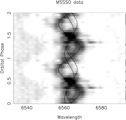
Figure 15: Left: Trailed SAAO spectra of the H$\alpha$ emission line, folded on the orbital ephemeris. Two cycles are shown for the sake of continuity, the second cycle being a copy of the first. Each spectrum was scaled so that the continuum just outside the H$\alpha$ profile is normalized to unity. The grey scale is chosen so that white corresponds to a value of 1 (i.e. the continuum) and black to 2.2 (the peak of the emission profiles in all spectra was 2.5). Orbital phase is shown on the ordinate axis and wavelength is shown on the abscissa. The curve labelled 2 corresponds to the expected motion of the M dwarf as deduced from the absorption line radial velocity curve derived above. The curve labelled 1 corresponds to the expected motion of the white dwarf as derived from the velocity variations in the HST spectra; the gamma velocity of 60 km s^-1 is included in curve 1. The curve labelled 3 corresponds to the motion of the feature in the Doppler tomogram at velocity co-ordinates (75, -75) km s^-1. It can be seem as a faint feature visible between orbital phase 0.6 and 0.9 and lying to the blue of the expected motion of the white dwarf. See text for more details. Right: As in the left panel except that the MSSSO data are shown.

From table 4.1 or fig. 4.13 of Reid & Hawley (2000), we derive a mean temperature for the M dwarf of $3100\pm 50$ K with intrinsic variation of semi-amplitude 75 K about this mean. Whether or not this variation is simply a function of orbital phase, or whether it is due, for example, to slowly migrating spotted regions on the surface of the M dwarf, will require far more data than is available in this study.

4.2.3 Rotational velocity of the M dwarf

Fig. 14b shows the same spectra as in Fig. 14a but with an expanded wavelength scale and a number of different rotational models. It is clear that both rotation and spectral type contribute to the depths of the lines. If GJ381 is used as the template, a rotational velocity of 150 km s^-1 is deduced. However, as shown in the last section, GJ381 is too early. The spectral fit to GJ273 (lower spectra) in parts of the wavelength range covered is too poor to judge the rotational velocity. No objective technique could be devised and inspection was resorted to. We conclude that the rotational velocity of the M dwarf is ${\rm V_{2}\ sin\ i\ =\ 125\pm 25\ kms^{-1}}$.

4.2.4 Metallicity of the M dwarf

With considerably subsolar metal abundances in the white dwarf, it is of some interest to determine the composition of the M dwarf. As illustrated in fig. 2.18 of Reid & Hawley (2000), chemical composition in M dwarfs is indicated by the increase in strength of the CaH compared to the TiO molecular bands as metal abundance decreases. Quantitative measurement is described by Gizis (1997); as shown by his fig. 1a, the distinction between disk M dwarfs on the one hand and subdwarfs or extreme subdwarfs on the other (with metal abundance of 1/16 solar or less) is clearest in the CAH1-TIO5 diagram. The measurements of these band indices rely on narrow band spectrophotometry and in order to reduce systematic uncertainties in our spectra of EC13471–1258, we measured these band strengths for three M dwarfs of similar spectral type (Table 10). As discussed above, for the M dwarf in EC13471–1258, a reasonably accurate subtraction of the spectrum of the white dwarf was required and additional uncertainty is associated with this.

The indices for the M dwarf in EC13471–1258 match those of the similar stars (all of which are normal disk M dwarfs); moreover, even after correcting for the systematic overestimation of the CAH1 index, it clear that the indices for the M dwarf in EC13471–1258 lie well away from the metal deficient M dwarf region in fig. 1a of Gizis (1997). We conclude that the M dwarf in EC13471–1258 has normal solar abundance and defer until later discussion of the considerably lower metal abundance in the white dwarf.

4.2.5 The behaviour of the emission lines

It was obvious even at the telescope that the profiles of the Balmer emission lines were comprised of more than one component; this constrained us from using them for radial velocity measurements as it would not be apparent how to interpret the results. We therefore folded all the SAAO highest resolution red spectra into 20 phase bins using the orbital ephemeris and scaled each in such a manner that the continuum just outside the H$\alpha$ emission line profile was normalized to unity. The results are shown as a trailed spectrum in the left panel of Fig. 15. The right panel shows the same procedure applied to the MSSSO data. Bearing in mind the worse resolution of the latter data, both panels are consistent with each other, indicating that the features seen are not transient but repeatable on a time scale of months.

The left panel shows that the H$\alpha$ emission line is indeed comprised of two components, leading to a doubling of the line profile at orbital phase 0.25, and a single peak at the phases of conjunction, 0.00 and 0.50. The stronger of the two components is well matched to the curve labelled 2; this curve is not a fit to this component but is instead the motion of the M dwarf derived from the absorption line radial velocity curve derived above.

Turning to the weaker of the two components, it is apparent that this varies around the orbital cycle, peaking in strength at orbital phase 0.20-0.25. At orbital phase 0.75, although much weaker in strength than half a cycle earlier/later, it is certainly present: examination of the individual spectra showed a clear doubling of the emission line in the orbital phase interval 0.60 to 0.70, disappearance of the weaker component around orbital phase 0.75, a brief reappearance at orbital phase 0.80 before merging with the redward moving stronger component at eclipse.

The curve labelled 1 corresponds to the expected motion of the white dwarf as derived from the velocity variations in the HST spectra, including its gamma velocity of 60 km s^-1. We are not convinced that this curve is a satisfactory description of the velocity variation of the weaker component in the data because it co-incides with no emission between orbital phase 0.70 and 0.85. Omitting the gamma velocity (which we attribute to a gravitational redshift from emission near the surface of the white dwarf), makes the fit worse. Whatever the case, the weaker component must originate on the same side of the binary centre of mass as the white dwarf as its curvature is clearly of opposite sign to that of the M dwarf’s motion.

We are convinced of the reality of the feature visible between orbital phases 0.60 and 0.90 just slightly to the blue of the curve labelled 1. The curve labelled 3 is derived from the Doppler tomogram discussed below. Note that its motion does not co-incide with the arc which is strongest between orbital phases 0.00 and 0.25 and which the curve labelled 1 passes through. Thus neither curves 1 nor 3 provide, on their own, a satisfactory representation of the weaker component.

It is also important to note the variations in strength of the stronger component. At phases close to conjunction, there is an obvious increase in strength which is plausibly explained by the summation of the two components. However, there is additional intrinsic variation in the strength of the stronger component: it weakens by at least a factor of two in the orbital phase interval 0.60-0.70 compared to the combined strength at orbital phase 0.50, and strengthens again suddenly at orbital phase 0.75. It is clear that the profile cannot be explained by the simple summation of two optically thin emission line sources of variable radial velocity. Turning briefly to the blue optical spectra (Fig. 17) which will be discussed more fully below, the relative fluxes in the Balmer emission lines shows that they are optically thick: the Balmer decrement is flat - the line strength ratios H$\alpha$/H$\beta$, H$\gamma$/H$\beta$, and H$\delta$/H$\beta$ are 1.4, 0.67 and 0.83, whereas Case B recombination predicts values of 2.80, 0.47 and 0.29, respectively (table 4 of Ferland et al. 1982). This provides a natural explanation for the intrinsic line strength variations in the H$\alpha$ profile: absorption of Balmer line photons by intervening gas is easily capable of explaining the variations seen. Specific scenarios in which this is taking place will be discussed later.

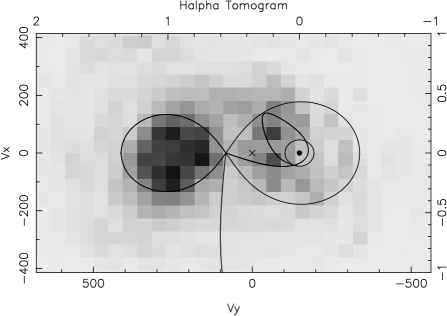
Figure 16: Left: Doppler tomogram of the H$\alpha$ emission line. Two scales are shown: velocity (lower horizontal and left vertical) and spatial (upper horizontal and right vertical). Both Roche lobes are shown as well as the binary centre of mass (cross), the white dwarf position (small filled circle) and the mass transfer stream in spatial co-ordinates as it loops around the white dwarf. The small circle surrounding the white dwarf is the inviscid disc radius (eq. 2.19 of Warner 1995). The Doppler map is scaled so that, in velocity co-ordinates, the M dwarf and white dwarf are at their correct respective positions (and by implication the Roche lobes are as well). The vertical line from the L1 point is the mass transfer stream in velocity co-ordinates. See text for discussion of the significance of all these features.

A Doppler tomogram (Marsh & Horne 1988) of the H$\alpha$ emission line in the SAAO data was calculated using the code of Spruit (1998). The results are shown in Fig. 16 which includes both velocity and spatial co-ordinates (the former on the lower horizontal and left vertical axes, the latter on the upper horizontal and right vertical axes). The origin of the spatial co-ordinates is the white dwarf and that of the velocity co-ordinates the binary centre of mass (depicted by a cross). The scales were adjusted, using the binary parameters adopted from later analysis, so that unity in the spatial system corresponds to ${\rm(K_{1}+K_{2})\ sin\ i}$ in the velocity system. The centre of mass of the M dwarf and the white dwarf are thus at their correct position in both co-ordinate systems, and so are the Roche lobes. We are aware that this implies that the velocity of any specific feature in the Doppler map arises only from the binary rotation and no other velocity component is included (e.g. the velocity of any streaming motions). Indeed, in velocity co-ordinates the mass transfer stream, as it moves away from the L1 point, quickly acquires ballistic velocities well in excess of the local binary rotation velocity and this is illustrated in Fig. 16 by the mass transfer stream whose velocity locus is the almost vertical line from the L1 point. Checks on the velocity of the stream shows that it never intersects the Roche lobe of the primary star.

With these considerations in mind, it is apparent that the majority of the emission arises from the vicinity of both Roche lobes. Further, the strongest emission component is centred on the Roche lobe of the M dwarf and has no bias towards or away from its inner hemisphere facing the white dwarf. This emission component corresponds to the line labelled ‘2’ in Fig. 15.

Within the white dwarf Roche lobe, the emission is biased towards the side facing the M dwarf and there are two distinct features at velocity co-ordinates (Vx, Vy) = (-25, -75) and (75, -75) km s^-1. The latter corresponds to the curve labelled ‘3’ in Fig. 15. The former feature does not fit the emission in the phase interval 0.0 to 0.25 as well as the curve labelled ‘1’ in Fig. 15. The interpretation of these two distinct features in the Doppler map is not straightforward. Neither occurs at a “special” place in the binary: e.g. neither feature is associated with the white dwarf. Furthermore, it is clear that while there is no accretion disc in the system of the kind seen in cataclysmic variables, there may be a very weak mass transfer stream flowing from the L1 point. In this case, one might expect features in the Doppler map corresponding to where this stream collides with itself. This could lead to an inviscid (i.e. dissipationless) disc which would be very hard to detect (see Warner 1995 and references therein for a discussion of inviscid discs within the context of disc formation). If there is, there might be a feature in the Doppler map corresponding to where the stream collides with such a disc. The radius of an inviscid disc is shown in Fig. 16 by the small circle around the white dwarf (eq. 2.19 of Warner 1995). One of the two distinct velocity features mentioned occurs near to, but not at, the intersection of the mass transfer stream with itself or the radius of an inviscid disc. The other feature is near to, but not at the place where the ballistic stream slows down to low velocities at the edge of its Roche lobe before plunging back for a second passage around the white dwarf.

We caution against expecting too much from the Doppler tomogram: the technique does not allow for intrinsic variations in emission line strength due to optical thickness in the lines (which are clearly present); moreover, there is some variation in the maps produced by spectra from each half of the orbital cycle (not shown). We are impressed that the emission line behaviour is not transient (it was seen in both the SAAO data on different occasions and in the MSSSO data). We believe that these results indicate the presence of streaming motions in the white dwarf Roche lobe implying the existence of mass transfer, albeit at a very low level. There is undoubtedly accretion on to the white dwarf from mass ejected by the M dwarf due to flares or its wind, i.e. not via the L1 point. Such accretion would not cause specific and stable features in the Doppler map. Clearly more data with at least double the resolution in wavelength and binary phase are required to elucidate these issues further.

In the right hand panel of Fig. 15, it is worth drawing attention to the additional emission occurring at orbital phase 0.35 and positioned to the red of the most redward motion of the M dwarf. Although these are phase folded spectra, the MSSSO data have only 3-4 spectra per bin on average and examination of the data that contribute to this phase bin show a clear triple structure to the emission line. Subsequent spectra showed the additional peak following the motion of the M dwarf indicating that the origin of the flare is close to that of the M dwarf and therefore attributable to the flaring behaviour noted above. There is also evidence for similar behaviour (but with the additional velocity component occurring in the extreme blue wings of the line) in some of the SAAO spectra from 1993 Apr 19/20. Flaring in the H$\alpha$ emission line has also been seen by Kawka et al. (2002).

The behaviour of the blue emission lines H$\beta$, H$\gamma$ and H$\delta$ was examined using the SAAO data from 1993 Feb and 1992 Apr 02/03, as well as the MSSSO data. The signal-to-noise in these data were generally much worse than in the H$\alpha$ data shown in Fig. 15; despite this, the behaviour of these features was consistent with that seen in H$\alpha$: a two-component profile with obvious doubling at phase 0.25 but with one component much weaker half an orbital cycle later.

The CaII K line’s behaviour was somewhat different in that it never showed doubling, was of lower velocity amplitude than the Balmer lines, and showed a strong variation around the orbital cycle with peak strength at orbital phase 0.5 and essentially disappearing at eclipse. This behaviour is strongly suggestive that this feature is formed on the inner hemisphere of the M dwarf facing the white dwarf.

Finally, the $H\alpha$ emission line was used to provide a more accurate estimate of the rotational velocity of the M dwarf than the absorption line value derived above. This is justified as it is clear from the Doppler tomography above that the velocity of the stronger component of the emission line is identical to that of the M dwarf. Fits of Doppler profiles to the emission line, and allowing for the instrumental resolution, yielded a value of V${\rm{}_{rot,2}\ sin\ i=140\pm 10}$ km s^-1.

Figure 17: The top curve is the sum of the blue spectra from 1992 Apr 02/03 and 1993 Feb. The bottom curve is the spectrum of the only M4.5eV star in the spectral atlas of Jacoby, Hunter & Christian 1984. The middle smooth curve is the white dwarf model fit from the HST data; the remaining middle curve is the difference between the top and bottom curves.

4.2.6 The blue spectra

The blue spectra from 1992 Apr 02/03 and from 1993 Feb were selected and summed together into 10 bins. Although the motion of the Balmer emission lines was obvious, no sign of the orbital motion of the white dwarf could be detected because the lines were too broad and the signal-to-noise ratio insufficient. Instead, the data were simply summed together and fluxed using the lower resolution spectrum in Fig. 2. The result is shown in Fig. 17 (top curve). It is clear that this spectrum is contaminated not only by Balmer emission but also by absorption features from the M dwarf, especially at the red end. We had no observations of M dwarfs in this spectral region, we could find no publicly available models with features to match the observations, so we made use of the observed spectrum of the M4.5eV star in the spectral atlas of Jacoby, Hunter & Christian (1984). Although its spectral type is 1 subclass later than that of the M dwarf in EC13471–1258, it was satisfactory for our purposes. A scaled version of this spectrum appears as the bottom curve in Fig. 17. The middle smooth curve shows the model for the white dwarf (T${}_{\rm eff}=14420$ K, log g = 8.34) along with the difference between the top and bottom curves. Allowing for subtraction uncertainties and instrumental effects, these two curves are a satisfactory match.

We tried to extract an independent estimate of effective temperature and gravity from the subtracted spectrum. This procedure was difficult as the emission cores had to be excluded and a fit to the continuum forced in several places. We decided that no reliable, independent estimate of the atmospheric parameters could be derived from this procedure. However, the solution was consistent within uncertainties with the HST value.

5 Analysis of the Binary

The numerical results from the previous analyses are listed in Table 12 along with their errors. Error estimates for some quantities, e.g. the eclipse analysis, are not shown as they are so small compared to the other error estimates that they can safely be neglected. A subset of these parameters allow derivation of the fundamental properties of the binary using the standard equations of spectroscopic binaries to derive the masses and radii of the individual components:

$${\rm a} = {\rm P_{orb}(K_{1}+K_{2})/2\pi}$$

$${\rm M} = {\rm 4\pi^{2}\ a^{3}/G\ P_{orb}^{2}}$$

$${\rm q} = {\rm K_{1}/K_{2}}$$

$${\rm M_{1}} = {\rm M/(1+q)}$$

$${\rm M_{2}} = {\rm q\ M_{1}}$$

$${\rm f(R_{1},R_{2},i)} = 0$$

$${\rm R_{lobe,2}/a} = {\rm 0.49q^{2/3}/(0.6q^{2/3}+ln(1+q^{1/3}))}$$

where a is the binary separation, M is the sum of the masses of the components, q is the ratio of the secondary to primary mass and ${\rm R_{lobe,2}}$ is the volume-equivalent Roche lobe radius of the secondary (Eggleton 1983).

Table 13: Summary of results

Quantity	Value	Error	Units
		Estimate
Porb	13025.5		s
f(r1/a, r2/a, i)	Table 3
Teff,1	14220	$\pm$350	K
log g	8.34	$\pm$0.22
log Z	-1.5	$\pm$0.5
K1 sin i	137	$\pm$10	km s-1
$\gamma_{1}$	61	$\pm$10	km s-1
Vrot,1 sin i	400	$\pm$100	km s-1
K2 sin i	266	$\pm$6	km s-1
$\gamma_{2}$	-2	$\pm$5	km s-1
Vrot,2 sin i	140	$\pm$10	km s-1
Teff,2	3100	$\pm$75	K

Figure 18: Mass-radius diagrams for the primary (lower panel) and secondary (upper) panel). The white dwarf mass-radius relation from Wood (1995) is shown in the lower panel labelled with ‘Wood’. Mass-radius relations for lower main sequence stars are shown in the upper panel: equation 2.99 of Warner (1995) is labelled ‘Warner’ and that derived in Clemens et al. (1998), based on Reid & Gizis (1997), is labelled ‘Clemens’. Each sloping line represents a solution for the binary using radial velocity semi-amplitudes indicated by the pair of numbers at the end of the corresponding line. Each dot along each line represents a one degree change in binary inclination; one line in each panel is labelled with the numerical value of the inclination. The 6-sided star on the white dwarf mass-radius relation represents the estimate of log g from the model atmosphere fitting to the HST data. In the upper panel, the dotted line represents the limit where the mean density of the M dwarf would exceed the Roche lobe mean density associated with that orbital period, and would therefore overfill the lobe. The mass derived from the gravitational redshift is 0.9 M_⊙; the vertical line in the lower panel is the acceptable mass range derived from the 1-$\sigma$ error estimate on the gravitational redshift. See the text for details of other features and additional discussion.

Measurements in Table 12 show values for K₁ sin i and K₂ sin i, not K₁ and K₂. As is well known in the analysis of spectroscopic binaries, although a is only dependent on K₁ sin i and K₂ sin i, M is dependent on the cube of these quantities. In the following analysis, therefore, uncertainties in the component masses and radii due to ignorance of the inclination and measurement errors in the radial velocity curves will be made explicit. The approach taken, therefore, was to try all integer values of i between 75^o and 90^o for the optimal values of K₁ sin i and K₂ sin i in Table 12, and to repeat the calculations for perturbations on the velocity semi-amplitudes using the error estimates in Table 12. Mass-radius diagrams showing the results of these calculations for each component appear in Fig. 18. Several lines appear in these diagrams which will require some explanation before discussing their significance:

• Consider first the lower panel (the white dwarf mass-radius diagram) and within this panel the line labelled with the numbers 266, 138. This line defines the locus of white dwarf mass-radius solutions for the optimal values of K₁ sin i and K₂ sin i from Table 12. Different inclination angles are shown as filled circles on this line. Larger filled circles are shown every five degrees along with a label showing the numerical value of the inclination. This line extends from 90^o (at the top) to 75^o.

• Lines parallel to the one just discussed are shown and represent solutions for the values of K₁ sin i and K₂ sin i indicated at the top of the line. In the upper panel corresponding lines are shown in the mass-radius diagram for the M dwarf. These loci will be referred to as “dynamic solutions”.

• In the lower panel the line labelled ‘Wood’ indicates the mass-radius relation for white dwarfs from the finite temperature, evolutionary models of Wood (1995). On this line is a 6-sided star which indicates the mass and radius of the white dwarf deduced from the value of log g combined with the Wood mass-radius relation. The uncertainty on the value of log g is indicated by showing the mass-radius relation as a solid line. Beyond the 1-$\sigma$ error interval, the mass-radius relation is shown as a dashed line.

• We interpret the difference between the $\gamma$ velocities of the white dwarf and M dwarf as arising from the gravitational redshift of the white dwarf. This directly translates into a white dwarf mass of 0.9 M_⊙. The uncertainty on the difference allows a lower mass estimate and the allowable interval (at the 1-$\sigma$ level) is indicated by the vertical line in the lower panel with the left pointing arrow attached and labelled ‘Gravitational Redshift’.

• As noted above, in the upper panel the dynamic solutions encompass a range of inclinations from 90^o to $\sim 75^{\rm o}$. At lower inclinations, the secondary would exceed its Roche lobe and are presumably excluded solutions. The parts of the dynamic solutions so excluded lie above the dotted line in the upper panel. This explains why the range of inclinations extended from 90^o to only 75^o. Note that the dotted line is essentially a geometric constraint, being based on the period-mean density relation for Roche lobe filling secondaries (see Warner 1995).

• Mass-radius relations for lower main sequence stars are shown in the upper panel: equation 2.99 of Warner (1995) is labelled ‘Warner’ and that derived in Clemens et al. (1998), based on Reid & Gizis (1997), is labelled ‘Clemens’.

• The remaining three almost horizontal lines in the upper panel, the leftmost of which is labelled ‘V_rot,2’, delineate a locus of M dwarf radii derived from the measurement of V_rot,2 sin i. The dependency on sin i is shown in the same manner as for the radial velocity lines which also define the corresponding value of M₂. Three lines are shown for three combinations of K₁ sin i and K₂ sin i.

Assuming that M dwarf radii in excess of the Roche lobe radius are excluded, the dynamic solutions representing the radial velocity semi-amplitudes and their $1-\sigma$ uncertainties, as well as the eclipse analysis, restrict the masses of the components to 0.59–0.83 and 0.30–0.45 M_⊙ for the white dwarf and M dwarf respectively. More precise values are available only if additional constraints are used.

The additional, purely observational constraints available are the loci of the M dwarf rotational velocity in the upper panel, and the gravitational redshift in the lower panel. The uncertainty on the M dwarf rotational velocity is 7 per cent or 1.5 carets on the ordinate axis of the upper panel. This restricts the range of allowable inclinations to less than 77^o. The gravitational redshift constrains the allowable range for the white dwarf mass to be larger than 0.8 M_⊙. The dynamic solutions impose a corresponding lower limit on the M dwarf mass to be larger than 0.43 M_⊙.

Inclusion of the Wood (1995) white dwarf mass-radius relation restricts the allowable inclinations to be smaller than 80^o.

Inclusion of the mass-radius relations for the M dwarf leads to interesting conclusions: (i) the relation in Warner (1995), which is typical of mass-radius relations from a number of sources, along with the assumption that the M dwarf radius does not overfill its Roche lobe, restricts the M dwarf mass to be smaller than 0.34 M_⊙. This is incompatible with the gravitational redshift constraint; (ii) Clemens et al. (1998) used the near infrared observations of Reid & Gizis (1997) to derive a mass-radius relation for M dwarfs, discovering an abrupt change in slope of the mass-radius relation as well as incompatibility with the mass-radius relations of the best theoretical models (see Reid & Hawley 2000 and references therein for a full discussion). The upper panel of Fig. 18 shows that the Clemens et al. relation, which diverges from the Warner and other “standard” relations at a secondary mass of 0.3 M_⊙, are compatible with the dynamical solutions for the M dwarf in EC13471–1258.

In arriving at a solution to the binary parameters, we attempted to achieve consistency with: (i) the M dwarf not overfilling its Roche lobe; (ii) the atmospheric parameter determination and Wood mass-radius relation for the white dwarf; (iii) the Clemens et al. mass-radius relation for the M dwarf (bearing in mind that there is intrinsic scatter in this relation); (iv) the V_rot,2 sin i determination for the M dwarf; (v) the gravitational redshift measurement; (vi) the dynamical solutions. In addition, we believe that the M dwarf is essentially filling its Roche lobe: evidence for this comes from the pre-eclipse dips (Fig. 8) without accompanying flare, and the specific features seen in the Doppler tomogram. If so, the solution will be on the dotted line in the upper panel of Fig. 18. Even if this is not the case, it is clear that the M dwarf is very close to filling its Roche lobe.

Accordingly, as the best “compromise” between all these constraints and their errors, we adopt an inclination of $75.5\pm 2.0^{\rm o}$, a white dwarf mass and radius of $0.78\pm 0.04$ M_⊙ and $0.011\pm 0.01$ R_⊙, and an M dwarf mass and radius of $0.43\pm 0.04$ M_⊙ and $0.42\pm 0.02$ R_⊙. We regard the error estimates as conservative. It is an endorsement of stellar evolution observation and theory that all the relevant constraints can be satisfied simultaneously.

5.1 Comparison with the results of Kawka et al.

Recently, Kawka et al. (2002) have reported observations and analysis of EC13471–1258 along with two other DA+dM systems. In general, their observational results broadly agree with those presented here. In the following parentheses, the results of Kawka et al. appear first, those presented in this paper second: the values of white dwarf log g (8.26, 8.34), T_eff (14080 K, 14220 K), and V_1,rot sin i (140 km s^-1, 140 km s^-1) are all consistent within the errors (though we are sceptical of their small error of 0.05 on log g, given the analysis of the error on this quantity shown above). There is, however, discord in the M dwarf radial velocity semi-amplitude ($241\pm 8.1$, $266\pm 6$). We are inclined to prefer our value as it was derived from the absorption features of the M dwarf and is also consistent with the motion of the stronger component of the emission lines.

The analysis of Kawka et al. is somewhat flawed in that they use the V sin i value to derive the absolute radius of the M dwarf without dependence on sin i. They then use the duration of the white dwarf eclipse along with the absolute radius of the M dwarf to derive the inclination (i.e. neglecting that this relationship also includes a, the orbital separation). Fortuitously, their inclination of 73.5^o is reasonable.

However, this inclination and, especially, the low value for the M dwarf radial velocity semi-amplitude yields a large value of 0.58 M_⊙ for the M dwarf mass. This, along with the M dwarf radius of 0.42 R_⊙ can be excluded for two reasons: (i) the radial velocity semi-amplitude for the white dwarf implied is about 185 km s^-1 (not 165 km s^-1 as claimed by Kawka et al.). This is excluded by the results in Table 8 and Fig. 12. Indeed, Kawka et al. derived a white dwarf radial velocity semi-amplitude of 155 km s^-1 but with large error (35 km s^-1), presumably because it seems from their fig. 11 that they used only one G140L HST spectrum from each orbit; (ii) the M dwarf mass and radius fall far from the locus of these quantities, either theoretical or empirical, derived from a large sample of M dwarfs (fig. 3 of Clemens et al. 1998; Reid & Gizis 1997). In addition, the spectral type implied by the M dwarf mass is M0 or earlier (see Reid & Hawley 2000) and discordant with the spectral type of M3.5-4 derived in this paper, or M2-M4 listed by Kawka et al. themselves. We believe that the M dwarf mass of Kawka et al. should be disregarded.

6 Discussion

6.1 Evolutionary status of the binary

The canonical theory for the formation of cataclysmic variables involves common envelope evolution enforcing dramatic orbital shrinkage with a hot white dwarf and an M dwarf emerging from the envelope of the AGB predecessor of the white dwarf. Following this, further orbital shrinkage takes place via angular momentum loss by the M dwarf through a weak wind with eventual contact. Further evolution of the semi-detached cataclysmic variable requires ongoing angular momentum loss to ensure ongoing Roche lobe contact by the M dwarf. These scenarios are discussed in Warner (1995) and references therein.

There is also an accumulation of evidence that the mass transfer rate in cataclysmic variables varies widely and perhaps cyclically on short time scales. Mass transfer may even shut off and the system “hibernates”, a term originated to explain the very existence of classical novae: in order to get a thermonuclear detonation with the vigour of those observed, the mass accretion rate was required to to be very low immediately before the nova explosion (Shara et al. 1986). The low mass accretion rate is now no longer believed to be so important (Prialnik & Kovetz 1995). More recent and direct evidence for variations in mass transfer rate is provided by the very wide range of mass transfer rates at a given orbital period evident in diagrams such as fig. 9.8 of Warner (1995). One hypothesis to explain such mass transfer rate variations is irradiation of the M dwarf by the white dwarf.

In terms of the above, therefore, EC13471–1258 is either a post common envelope binary just at the phase where its M dwarf comes into contact with its Roche lobe for the first time, or it is a system that has been in contact and is currently hibernating. We believe that two pieces of evidence favour the latter interpretation:

• the rotational velocity of the white dwarf: with V${}_{\rm rot,1}=400\pm 100$ km s^-1, the star rotates in 120 s. Such a rapid rotation rate implies that there has been an earlier phase of spin-up by mass transfer. Indeed, inspection of table 4 of Szkody et al. (2002a) shows that this rotation velocity is typical of cataclysmic variables.

• the behaviour of the H$\alpha$ emission line profile: although the interpretation of the Doppler tomogram is not clear, what is clear is that there are two or more components in the emission line and intrinsic variability as well, even in the component associated with the M dwarf. As the Balmer lines are optically thick, it is clear that the intrinsic variability can be understood by absorption by gas in the Roche lobe of the primary. The fact that the variation is a function of binary phase indicates that the absorption sites are fixed in the rotating reference frame of the binary and hence that there is a very weak mass transfer stream.

We therefore conclude that EC13471–1258 is a hibernating cataclysmic variable.

Interestingly, the white dwarf temperature in EC13471–1258 is cool compared to white dwarfs in cataclysmic variables of similar orbital period. Indeed the temperature of this white dwarf is more typical of systems below the period gap (fig. 3 of Szkody et al. 2002a). It is close to the temperature of the pulsating white dwarf in GW Lib (Szkody et al. 2002b), but shows no oscillations.

The white dwarf radius and model atmosphere imply a distance to the system of $48\pm 5$ pc, well within the reach of ground-based parallax programs. An accurate parallax would enable a more stringent test of the white dwarf mass-radius relationship than presented in this paper. An absolute V magnitude of the white dwarf was derived: 11.74.

6.2 The M dwarf

The analysis of the M dwarf presented in this paper shows that its properties are compatible with field stars of similar spectral type. This M dwarf is of particular relevance to studies of M dwarfs of the kind conducted by Reid & Gizis (1997) and Clemens et al. (1998) as its properties (V-I colour, mass and radius) place it in the segment of the M dwarf sequence where an abrupt change in slope of many stellar parameters occurs. This abrupt change in slope is discussed in Clemens et al. (1998) and Reid & Gizis (1997) to which the reader should turn for further information.

The M dwarf exhibits the properties expected of a secondary star in a cataclysmic variable: it is extremely active, presumably because of its very short rotation period. The erratic behaviour of the binary period is also typical of cataclysmic variables and presumably arises from magnetic cycling in the M dwarf (e.g. Warner 1995 and references therein). If flares of the kind described in this paper occurred on the secondaries of cataclysmic variables with higher mass transfer rate, they would be indistinguishable from the flickering in the system.

Compatibility with the Clemens et al. mass-radius relation implies that the M dwarf is 250 K hotter than the 3100 K derived above: see fig. 4.13 of Reid & Hawley (2000). As they discuss, the temperature scale for M dwarfs is uncertain by this amount. Resolution of this discrepancy must await further developments in M dwarf model atmosphere research.

A puzzling feature of the photometry of the M dwarf is the fact that the ellipsoidal variation is not constant and is often asymmetrical with respect to the conjunction of the two stars. When this happens, its minimum occurs slightly before orbital phase 0. If this behaviour could be attributed to star spots on the M dwarf, it would not be puzzling. However, spots on other chromospherically active stars migrate. In this case, 10 years of eclipse monitoring has shown that the asymmetry is either absent or always in the same sense.

Using the distance derived from the last subsection, the absolute V magnitude of the M dwarf is 11.82.

6.3 Chemical composition of the binary components

The chemical compositions of the binary components are different: that of the M dwarf is normal solar, that of the white dwarf is 1/30 solar. As has been well known for decades, the chemical composition of the photospheres of typical single DA white dwarfs is extremely metal deficient ($<10^{-6}$) due to gravitational settling of heavy elements in the very high surface gravity of the white dwarf. The presence of metals in the white dwarf in EC13471–1258, therefore, is due to mass accretion from the nearby M dwarf (whether this mass transfer is from the wind of the M dwarf or Roche lobe overflow is not relevant to this discussion). Metals are also seen in the white dwarf primaries of cataclysmic variables where sub-solar metal abundances are common (see table 4 of Szkody et al. 2002a). The abundances nevertheless vastly exceed the abundances in single white dwarfs.

If the chemical composition difference is in steady state, and the mass accretion rate on to the white dwarf can be estimated, the diffusion coefficients for the chemical species visible in the HST spectra can be deduced. This is beyond the scope of this paper but is clearly an interesting avenue for future work as this system provides a natural diffusion laboratory.

Acknowledgements

DOD thanks Ed Sion for a heroic attempt to observe this star with IUE. We are grateful to Xavier Delfosse for supplying the radial velocity of GJ381, to Hans Ritter, Andrew King, Boris Gansicke, Brian Warner and Mike Shara for helpful conversations, to Henk Spruit for the use of his Doppler tomography software, and to Steve Potter for help with its implementation. This paper has had an even longer gestation period than that of O’Brien, Bond & Sion (2001); DOD thanks Kawka and collaborators for what some of his co-authors and colleagues tried for so long to exert: pressure to finish the paper.

References

- [] Allard N.F., Koester D., 1992, A&A, 258, 464
- [] Bessell M.S., 1979, PASP, 91, 589
- [] Bessell M.S., 1990, A&AS, 83, 357
- [] Clemens J.C., Reid I.N., Gizis J., O’Brien M.S., 1998, ApJ, 496, 352
- [] Delfosse X., Forveille T., Benzit J.-L., Udry S., Mayor M., Perrier C., 1999, A&A, 344, 897
- [] Eggleton P.P., 1983, ApJ, 268, 368
- [] Ferland G., Lambert D.L., McCall M.L., Shields G.A., Slovak M.H., 1982, ApJ, 260, 794
- [] Finley D.S., Koester D., Basri G., 1997, ApJ, 488, 375
- [] Gizis J.E., 1997, AJ, 113, 806
- [] Hamuy M., Suntzeff N.B., Heathcote S.R., Walker A.R., Gigoux P., Phillips M.M., 1994, PASP, 106, 566
- [] Hawley S.L., Gizis J.E., Reid I.N., 1996, AJ, 112, 2799
- [] Hawley S.L., Reid I.N., Gizis J.E., 2000, in “From Giant Planets to Cool Stars”, eds. C.A. Griffiths and M.S. Marley, ASP Conf. Ser. 212, 252
- [] Homeier D., Koester D., Hagen H.-J., Jordan S., Heber U., Engels D., Reimers D., Dreizler S., 1998, A&A, 338, 563
- [] Jacoby G.H., Hunter D.A., Christian C.A., 1984, ApJS, 56, 257
- [] Kawka A., Vennes S., Koch R., Williams A., 2002, AJ, 124, 2853
- [] Kilkenny D., Koen C., O’Donoghue D., Stobie R.S., 1997, MNRAS, 285, 640 (Paper I)
- [] Kirkpatrick J.D., Henry T.J., McCarthy D.W., 1991, ApJS, 77, 417
- [] Koen C., 1996, MNRAS, 283, 671
- [] Koen C., Kilkenny D., van Wyk F., Cooper D., Marang F., 2002, MNRAS, 334, 20
- [] Marsh T.R., Horne K.D., 1988, MNRAS, 235, 269
- [] Menzies J.W., Cousins A.W.J., Banfield R.M., Laing J.D., 1989, SAAO Circ., 13, 1
- [] Nidever D.L., Marcy G.W., Butler R.P., Fischer D.A., Vogt S.S., 2002, ApJS, 141, 503
- [] O’Brien M.S., Bond H.E., Sion E.M., 2001, ApJ, 563, 971
- [] Press W.H., Teukolsky S.A., Vetterling W.T., Flannery B.P., 1992, Numerical Recipes in FORTRAN, 2nd Edition, Cambridge University Press, Cambridge.
- [] Prialnik D. & Kovetz A., 1995, ApJ, 445, 789
- [] Reid I.N., Hawley S.L., 2000, New Light On Dark Stars: Red Dwarfs, Low-Mass Stars, Brown Dwarfs, Praxis, Chichester
- [] Reid I.N., Hawley S.L., Gizis J.E., 1995, AJ, 110, 1838
- [] Reid I.N., Gizis J.E., 1997, AJ, 113, 2246
- [] Ritter H., Schroder R., 1979, A&A, 76, 168
- [] Robinson E.L., Nather R.E., Patterson J., 1978, ApJ, 219, 168
- [] Shara M.M., Livio M., Moffat A.F.J., Orio M., 1986, ApJ, 311, 163
- [] Spruit H.C., 1998, astro-ph/9806141
- [] Stobie R.S., et al., 1997, MNRAS, 287, 848
- [] Szkody P., Sion E.M., Gansicke B., Howell S.B., 2002a, The Physics of Cataclysmic Variables and Related Objects, ASP Conference Series vol. 261, 21
- [] Szkody P., Gansicke B., Howell S.B., Sion E.M., 2002b, ApJ, 575, L79
- [] Tonry J., Davis M., 1979, AJ, 84, 1511
- [] Unsöld A., 1968, Physik der Sternatmosphären, Springer-Verlag Berlin, Heidelberg, New York, p.508
- [] Warner B., 1995, Cataclysmic Variable Stars, Cambridge University Press, Cambridge
- [] Wood M.A., 1995, Lecture Notes in Physics, Vol. 443: White Dwarfs, 41