The Environment of AGNs in the Sloan Digital Sky Survey

Abstract

We present the observed fraction of galaxies with an Active Galactic Nucleus (AGN) as a function of environment in the Early Data Release of the Sloan Digital Sky Survey (SDSS). Using 4921 galaxies between $0.05\leq z\leq 0.095$, and brighter than ${\rm M_{r^{*}}}=-20.0$ (or ${\rm M^{\star}}+1.45$), we find at least $\sim 20\%$ of these galaxies possess an unambiguous detection of an AGN, but this fraction could be as high as $\simeq 40\%$ after we model the ambiguous emission line galaxies in our sample. We have studied the environmental dependence of galaxies using the local galaxy density as determined from the distance to the $10^{th}$ nearest neighbor. As expected, we observe that the fraction of star–forming galaxies decreases with density, while the fraction of passive galaxies (no emission lines) increases with density. In contrast, the fraction of galaxies with an AGN remains constant from the cores of galaxy clusters to the rarefied field population. We conclude that the presence of an AGN is independent of the disk component of a galaxy. We have extensively tested our results and they are robust against measurement error, definition of an AGN, aperture bias, stellar absorption, survey geometry and signal–to–noise. Our observations are consistent with the hypothesis that a supermassive black hole resides in the bulge of all massive galaxies and $\simeq 40\%$ of these black holes are seen as AGNs in our sample. A high fraction of local galaxies with an AGN suggests that either the mean lifetime of these AGNs is longer than previously thought (i.e., $\geq 10^{8}$ years), or that the AGN burst more often than expected; $\sim 40$ times over the redshift range of our sample.

1. Introduction

A fundamental goal of observational cosmology is to determine the spatial distribution of galaxies as a function of galaxy properties, e.g., luminosity, morphology, star formation rate etc., as such observations place constraints on models of galaxy formation and evolution. In recent years, there has been an explosion in such work due to improvements in the theoretical modeling of galaxy evolutionary processes (e.g., Kauffmann et al. 1999; Benson et al. 2002) and the availability of large amounts of high quality survey data, e.g., Sloan Digital Sky Survey (SDSS; York et al. 2000), 2dF Galaxy Redshift Survey (Colless et al. 2001), Las Campanas Redshift Survey (Shectman et al. 1996) and the Century Survey (Wegner et al. 2001).

In this paper, we focus on one aspect of such research, namely the relation between the fraction of local galaxies that possess an Active Galactic Nucleus (AGN) and the local environment of those galaxies. Such observations can provide new constraints on models of galaxy evolution (e.g., how the AGN may affect other galaxy properties like star–formation), as well as providing insights into the physical mechanism(s) powering the AGN. For example, an AGN could be fueled by the same cold gas in the disk component of galaxies that is driving the star–formation rate (SFR) of those galaxies. In this case, the existence of an AGN might diminish in dense regions, analagous to the SFR-density relation (see Lewis et al. 2002; Gomez et al. 2003, Carter et al. 2001). Alternatively, several authors have proposed that galaxy–galaxy collisions fuel the AGN activity by driving gas into the cores of galaxies and thus onto the black hole (Gunn 1979; Shlosman 1990). A third possible empirical model proposed by Kormendy & Gebhardt (2001) suggests that supermassive black holes are solely a bulge phenomena and were formed at the same time as the bulge component of galaxies at an much earlier epoch in the Universe. In this model, the distribution of AGNs would then trace the distribution of bulges, under the assumption that AGNs are powered by supermassive black holes (Lynden–Bell 1964).

Therefore, by studying the fraction of galaxies that possess an AGN, as a function of environment, one can obtain constraints on such models of AGN activity and formation. Observationally, the fraction of galaxies with an AGN has increased as the quality and quantity of the spectral data has improved. In the early work of Dressler, Thompson, & Shectman (1985), they found that only a few percent of galaxies possessed an AGN (see also Huchra & Burg 1992), and there were approximately five times as many AGNs in the field compared to the cores of clusters. In recent years, Carter et al. (2001; CFGKM hereafter) measured an AGN fraction of 17%, while Ho, Fillipenko & Sargent (1997) find an AGN fraction of $\sim 40\%$ (this difference depends upon the details of the spectral definition of an AGN). Furthermore, there is now less evidence for an environmental dependence on the AGN fraction (see CFGKM).

Herein, we present the AGN–density relation for galaxies in the Early Data Release (EDR) of the Sloan Digital Sky Survey (SDSS). This relation is analogous to the SFR–density (Hashimoto et al. 1998, CFGKM) and morphology–density (Dressler et al. 1980; Postman & Geller 1984; Dressler et al. 1997) relations we have presented elsewhere in Gomez et al. (2003) and Goto et al. (in prep.) respectively. The work presented herein builds upon earlier studies of the spectral properties of galaxies as a function of environment (e.g., CFGKM, Tresse et al. 1999, Loveday et al. 1999). In Section 2, we discuss the data and techniques used for identifying an AGN in the SDSS galaxies. In Section 3, we present our results on the AGN–density relation, while in Section 4, we discuss these results and their physical implications. We conclude in Section 5. Throughout this paper, we used ${\rm H_{o}}=75{\rm km\,s^{-1}\,Mpc^{-1}}$ and $\Omega_{matter}=0.3$ and $\Omega_{\Lambda}=0.7$.

2. The Data

The data are taken from the Early Data Release of the SDSS (see Stoughton et al. 2002; see also Blanton et al. 2003; Fukugita et al. 2003; Gunn et al. 1998; Hogg et al. 2001; Pier et al. 2003; Smith et al. 2002; Strauss et al. 2002). One of the unique features of the SDSS is the sophisticated data analysis software pipelines used to reduce the raw images and spectra into large catalogs of sources and measured properties. Briefly, for each flux–calibrated SDSS spectrum, a redshift is determined from both the absorption lines, via cross-correlation, and the emission lines, via a wavelet–based peak–finding algorithm (see Frieman et al. in prep). Once the redshift is known, the spectroscopic pipeline estimates the continuum emission at each pixel by using the median value seen in a sliding box of 100 pixels centered on that pixel. Emission and absorption lines are measured by fitting a Gaussian, above the continuum, at the redshifted rest–wavelength of the lines. In order to avoid line blending, the SDSS pipeline fits multiple Gaussians in such cases as [NII]  and H$\alpha$ . Thus, the spectroscopic pipeline provides a high quality estimate of the equivalent width (EW), continuum, rest–wavelength, identification, goodness–of–fit ($\chi^{2}$), height and sigma (and the associated errors on these quantities) for all the major emission and absorption lines in galaxy spectra. This extensive emission and absorption line database, when combined with color and morphological information from the SDSS photometric survey, is ideal for studying the properties of low redshift galaxies.

The galaxy sample we use is similar to the one described in Gomez et al. (2003). Briefly, we define a pseudo volume-limited sample by restricting the analysis to galaxies in the redshift range $0.05\leq~{}z\leq 0.095$, and to galaxies more luminous than a (k–corrected; Blanton et al. 2002) $M(r^{*})=-20$ which is $M^{\star}(r^{*})-1.45$ assuming $M^{\star}{r^{*}}~{}=~{}-20.8+5\log{h}$ from Blanton et al. (2001). The lower redshift limit is to minimize aperture bias (see Gomez et al. 2003 and Section 2.6) due to large nearby galaxies, while the upper redshift limit corresponds to where luminosity limit equals the apparent magnitude limit of the SDSS ($r^{*}=17.77$; Strauss et al. 2002).

2.1. Survey Edges

The SDSS EDR covers a contiguous area of $\simeq 400$ square degrees with a complicated geometry. Much of the area is contained within two long stripes that are $2.5$ degrees wide in declination, centered on the celestial equator. Thus, many of the galaxies in the EDR are close to a survey boundary. This geometry requires that careful attention be paid to any measure of local galaxy density measurements. We have chosen to use the distance to the 10^th nearest neighbor (see Section 3) to infer local densities.

To avoid a biased density measure, we have excluded galaxies that have a survey edge closer than the distance to the 10^th nearest neighbor. We have tested this method of “edge correction” using the mock galaxy catalogs of Cole et al. (1999). We used these data to create a mock galaxy catalog with the same geometry as the SDSS EDR, and then measure the projected distance to the 10^th nearest neighbor in the full mock (i.e., without edges) and within the catalog with the EDR geometry. Our results are shown in Figure 1, which shows that if we ignore edges, the measured distance to the 10^th nearest neighbor is biased towards higher values compared to the true 10^th nearest neighbor distance. However, as expected, once we remove all galaxies which have an edge closer than the 10^th nearest neighbor, we then recover the true distances, or local densities. Figure 1 shows the importance in correctly accounting for edges in surveys with complicated volumes, such as the SDSS EDR.

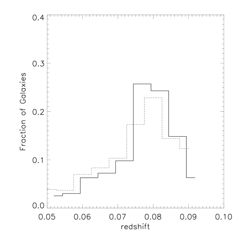
We note that while the edge correction produces an unbiased estimate of the density (as shown in Figure 1), the distribution of densities for our sample is different than the whole EDR survey. In Figure 2, we plot the redshift histogram of our sample before and after the edge correction is made. The edge correction results in a smaller survey area (than the whole EDR) at the lowest redshift, as the volume sampled at $z\simeq 0.05$ is small compared to the typical distance to the 10^th nearest galaxy neighbor). Additionally, since galaxies in dense environment have closer neighbors than galaxies in voids, we preferentially sample dense regions more often than sparse regions; we note however that the signal-to-noise of the measured densities is independent of this effect as we alway use 10 galaxies to define the local galaxy density.

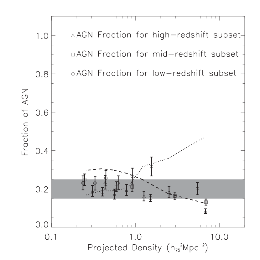
Our results are robust against this bias in the distribution of densities for two reasons. First, we only study herein the fraction of galaxies as a function of the various galaxy types (i.e., AGN, star-forming and passive) and have binned the galaxies in density such that each bin has $\simeq 250$ galaxies per bin (this changes slightly for the analyses as a function of redshift). Therefore, higher density regions are more finely binned compared to lower density regions. Secondly, we have divided our sample into three nearly equal volume subsets, as a function of redshift, and show that our conclusions are independent of redshift (see Figure 9). This suggests that the bias seen in Figure 2 is unimportant. In summary, our tests show that we possess an unbiased estimate of the local (projected) galaxy density over two orders of magnitude in the density, i.e., from $\sim 10{\rm h_{75}^{2}}\,{\rm Mpc^{-2}}$ to $\sim 0.1{\rm h_{75}^{2}}\,{\rm Mpc^{-2}}$ (see Figure 1). Our final, edge-corrected sample, contains 4921 galaxies with a mean spectral signal-to-noise ratio for their spectra of 24. The wavelength coverage is 3900Å  to 9100Å, with a spectral-resolution of 1800.

We note here that there are 27 sources spectrally classified by the SDSS software pipeline as quasars within the sample limits defined above. These 27 low redshift QSOs (which are actually Seyfert Type I AGNs) possess extremely broad lines making it difficult to obtain line flux-ratio measurements (especially for [NII]  and H$\alpha$  which lie only 20Å  apart). We note that a Kolmogorov-Smirnov test indicates no difference between the environments of these low-z QSOs and of our AGN sample defined in Section 2.2. Therefore, as there are so few of these objects (0.5% of our total sample), and they exist in the same environments as our full AGN sample (of nearly 1000 galaxies), we ignore these QSOs unless otherwise noted.

2.2. Identifying AGNs: Part I

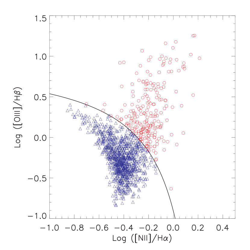
To classify AGNs, we use the traditional log([OIII]/H$\beta$) versus log([NII]/H$\alpha$) flux-ratio diagnostic diagrams as discussed by Baldwin, Philips & Telervich (1981), Villieux & Osterbrock (1987) and Kewley et al. (2001). The flux of these emission lines are determined using the fitted heights and sigmas of the lines as measured by the SDSS data analysis pipeline. We initially restrict our analysis to lines with a measured flux over flux error of $>2$, i.e., $>2\sigma$ detections. In Figure 3 (left), we show the model (solid line) used to separate star–forming galaxies from AGNs. Galaxies which lie above, and to the right of, this model are classified as AGNs, while galaxies beneath, and to the left, are classified as star–forming galaxies.

For the 4921 galaxies in our pseudo volume-limited sample, 3647 have at least one $>2\sigma$ emission line detection, while 1293 galaxies have all of the four lines required in Figure 3 for an unambiguous classification (e.g., the [NII], [OIII], H$\alpha$  and H$\beta$  emission lines). Most of the galaxies with these four emission lines (82%) are classified as star-forming galaxies. These star-forming galaxies have a median H$\alpha$  equivalent width (EW) of 26Å. The remaining 235 galaxies are classified as AGNs with a median H$\alpha$  EW of 13Å. We call these the “4–line AGNs” for the rest of the paper. We have made no attempt to classify these AGNs into sub–populations like LINERs, Seyferts I or II. We simply note that these 235 AGNs do cover a broad range of AGN types. Likewise, we have made no attempt to study the individual properties of the AGNs.

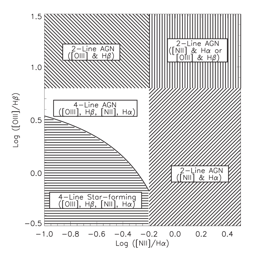
We note here that it is not necessary to possess significant detections of all four of these lines ([NII], [OIII], H$\alpha$  and H$\beta$) to unambiguously detect an AGN in a galaxy; although one does need all four lines to unambiguously classify star-forming galaxies. We illustrate this fact in Figure 4, which shows that galaxies with either a high [NII]/H$\alpha$ , or a high [OIII]/H$\beta$ , line ratio must be an AGN (see CFGKM), regardless of the other line ratio. [We note that we find no AGNs using solely the [OIII]/H$\beta$  line ratio]. Star–forming galaxies only inhabit the bottom left–hand corner of Figure 3. For example, if a galaxy has [NII]  and H$\alpha$  lines detected at $>2\sigma$ confidence, but no significant detection of [OIII]  or H$\beta$, we can still classify it as an AGN if log([NII]/H$\alpha$)$>-0.2$. Carter et al. (2001) used a similar technique to extract additional AGNs in their data. To differentiate these AGNs from the 4–line AGNs discussed above, we call these AGNs “2–line AGNs”, as they are classified using only two lines. These “2–line AGNs” have much lower line strengths than the “4–line AGNs”, as they possess a median EW of H$\alpha)\simeq 3$. However, there is no difference in the signal-to-noise ratios of the “2–line” AGN spectra compared to “4–line” AGN spectra. In Figure 5, we show the [NII]/H$\alpha$  flux-ratios for these 2–line AGNs.

Using log([NII]/H$\alpha$)$>-0.2$, we have increased our AGN sample from 235 (4–line AGNs) to 936 galaxies. Thus, the majority of our AGNs are classified using only the [NII]  and H$\alpha$  lines, which has two important advantages compared to the 4–line method. First, the classification is unambiguous, since we have chosen line ratios high enough to exclude nearly all star–forming galaxies in Figure 1. Second, [NII]  and H$\alpha$  are close together in wavelength so we have no concerns about the amount of internal dust extinction when classifying these galaxies.

There remains a large number of galaxies that have at least one $>2\sigma$ detection of an emission line, but cannot be classified using either the 2–line or 4–line method discussed above. We call these galaxies “Emission Line but Unclassified” (ELU) galaxies. We discuss these further in Section 3.1. Any galaxy with no $>2\sigma$ detected emission lines is classified as “passive”. In Table 1, we present the fraction of galaxies as a function of these different classifications.

2.3. Identifying AGNs: Part II

To study the effect of measurement errors (see CFGKM), we apply a different classification technique to our sample, which utilizes the observed error on the line ratios, and calculates the probability that each galaxy is either star–forming or contains an AGN. The method uses the False Discovery Rate (FDR) described in Miller et al. (2001) and has the advantage of controlling the amount of contamination in each class of galaxies, which is the scientifically meaningful quantity. For our FDR technique, we drop the requirement that all lines must be detected at the $>2\sigma$ confidence level, and instead use all lines that have a positive value (i.e., emission) regardless of their measurement error.

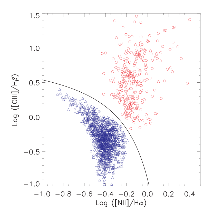
To use FDR, we must begin by assuming a null hypothesis and test each galaxy against that null hypothesis. Our first null hypothesis is to assume that any galaxy below the model line shown in Figure 3 is a star–forming galaxy, i.e., it has a probability of 1 of being star–forming. Then, for all galaxies above the line in our sample, we assign a probability of being star–forming assuming the errors on the line ratios are Gaussian. Once we have a probability for each galaxy, we use FDR to reject galaxies from this null hypothesis (i.e., they are AGNs) at a confidence level of 90%. Therefore, we obtain a sample of AGNs that is guaranteed to have less than 10% contamination from star-forming galaxies. We then alter our null hypothesis, so that all galaxies above the model line in Figure 3 are classified as AGNs, and re–calculate the probability for each galaxy below the line. Once again we use FDR to control the false detection rate and obtain a sample of star–forming galaxies that are rejected based on this new null hypothesis. Again, this guarantees fewer than 10% contamination by AGNs in our sample of star–forming galaxies. This procedure produces a robust sample of star–forming and AGN classifications, as well as galaxies that are unclassified because they were rejected against both null hypotheses.

In Figure 3 (right) we plot the flux ratio diagnostic diagram constructed using the FDR method described above. In this figure, all galaxies with line ratios close to the model separating AGNs and star–forming galaxies are unclassified. The FDR classification scheme (which properly treats the errors on the line-fluxes and ratios) picks up more AGN with weak lines (i.e. some less than 2$\sigma$) at the expense of missing “transition galaxies” which have evidence of both star-formation and an AGN. Overall, the FDR method is more conservative than the the $>2\sigma$ line method described in Section 2.2. However, we still find a similar fraction of AGNs and star–forming galaxies as we did when simply requiring all lines were detected at the $>2\sigma$ confidence. For example, the total number of 4–line and 2–line AGNs we calculate using the FDR method is similar to that found using the $>2\sigma$ method; 14% for FDR compared to 19% in Table 1.

2.4. Low-Luminosity AGNs

The SDSS spectroscopic analysis pipeline (see Section 2) determines the location and flux of an emission line via a Gaussian fit to the spectral data. This fit does not account for the possibility of stellar absorption which would lie underneath any emission line. Such absorption could lead to a systematic uncertainty in the measured flux of the hydrogen emission lines in the SDSS spectra (see Gomez et al. 2003; Goto et al. 2003). To overcome such problems, several authors (Ho, Fillipenko, Sargent 1997; Coziol et al. 1998) have advocated using template spectra to estimate the amount of stellar absorption underneath the hydrogen lines. Such a technique involves fitting the continuum flux of each galaxy spectrum with these templates and finding the best fit. Then, the emission lines are measured taking into account the expected amount of stellar absorption as seen in the best–fit template spectrum. This technique has the advantage of being more sensitive to lower luminosity AGNs (LLAGNs), as one is able to identify and measure the weaker emission lines. This, in part, explains why Ho, Fillipenko, Sargent (1997) and Coziol et al. (1998) find more AGNs than previous studies who did not use template fitting techniques.

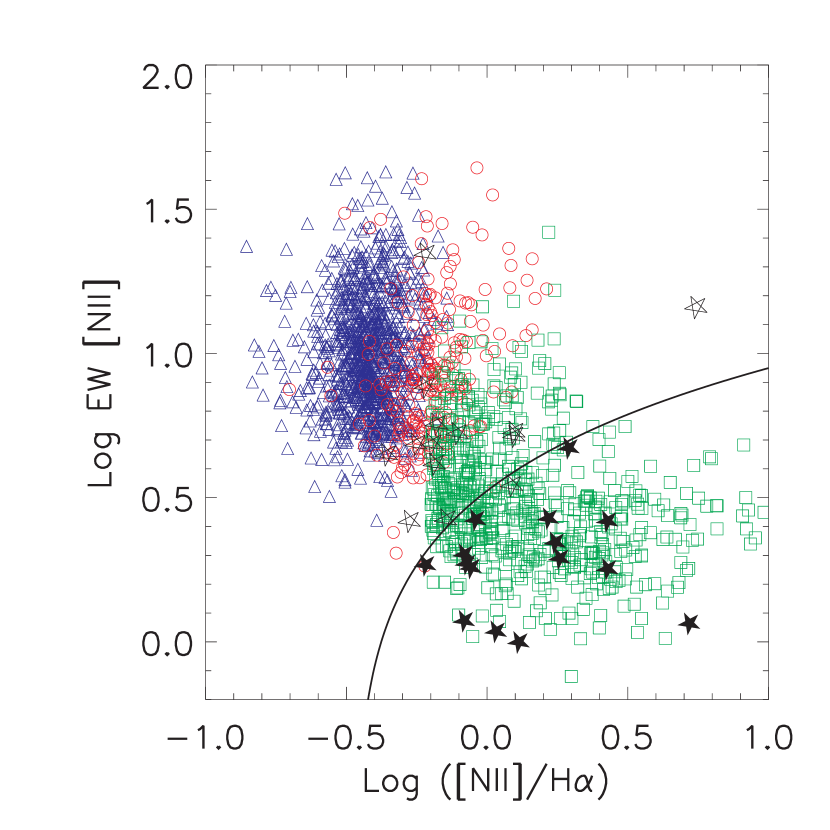
We examine here the issue of low luminosity AGNs and test our ability of finding such sources using our AGN identification techniques as discussed in Section 2.2. As a basis for our tests, we compare our analysis with the sample of 82 Hickson group galaxies studied by Coziol et al. (1998), who used the template fitting technique to study the LLAGN population in groups of galaxies. As we see no dependence on the AGN fraction with environment (see Section 3), the environment of the Coziol et al. sample is irrelevant and does not bias our tests. In Figure 5, we present the observed rest-frame equivalent width of [NII]  for galaxies in our sample as a function of their observed [NII]/H$\alpha$  line ratio. Only galaxies with $>2\sigma$ detections of both the [NII]  and H$\alpha$  lines are shown here. Figure 5 is therefore similar to Figure 5 in Coziol et al. (1998), who use such a diagram as a diagnostic to indicate the separation between star–forming galaxies, AGNs and LLAGNs.

We find a significant population of our 2–line AGNs are LLAGNs, as they possess weak [NII]  and H$\alpha$  emission lines, e.g., only a few Å  of EW in these detected lines. This is because of the high resolution of the SDSS spectra (2.3Å  per resolution element), which helps de–blend the [NII]  doublet and H$\alpha$  emission lines, and the high mean signal–to–noise ratio (S/N$=23.9$) of our LLAGN spectra. Therefore, we have the sensitivity to detect any strong [OIII]  and H$\beta$  emission in these spectra if it was present. In summary, most of our 2–line AGN detections are LLAGNs, as by definition they possess weaker [NII]  and H$\alpha$  emission lines (but with a large line ratio), and no detectable [OIII]  and H$\beta$  emission.

We note here that we find no correlation between our H$\alpha$  fluxes and the signal-to-noise of the spectra. In other words, it is not the case that all of our low H$\alpha$  flux galaxies have low S/N spectra (and thus large errors).

2.5. Effects of Stellar Absorption

Our ability to detect LLAGNs (discussed above) and our agreement with Coziol et al. (1998) indicates that our method can accurately classify AGNs without the need for template fitting. To expand on this, we have performed two tests quantify the effect of stellar absorption on our classifications.

First, we have visually inspected the profiles of the [NII]  and H$\alpha$  emission lines in the spectra of the 50 AGNs with the smallest H$\alpha$  equivalent widths that are close to the model line in Figure 5. Using the absorption in H$\beta$  as an upper limit to the total possible stellar absorption in the galaxy, we conclude that $\sim 5$ of these 50 galaxies could change classification from AGN to star-forming. These inspections demonstrate that only $10$% of these lowest luminosity AGNs are affected by stellar absorption. Second, we add 0.7Å  of stellar absorption to all the hydrogen lines in our spectra and re-classified them. This mean amount of stellar absorption has been estimated by Hopkins et al. (in prep) to obtain consistent measurements of the SFR of SDSS galaxies using H$\alpha$, [OII], $u^{\prime}$-band luminosity, with the IRAS infrared luminosities and radio luminosities from the FIRST survey. After applying this absorption correction, our total fraction of AGNs changes from 19% (in Table 1) to 17%. We conclude from both of these tests that our final sample of “2–line” and “4–line” AGNs is robust against stellar absorption corrections. Since we are not attempting to measure precise line fluxes in this work, we ignore stellar absorption throughout the rest of this work.

2.6. Aperture Effects

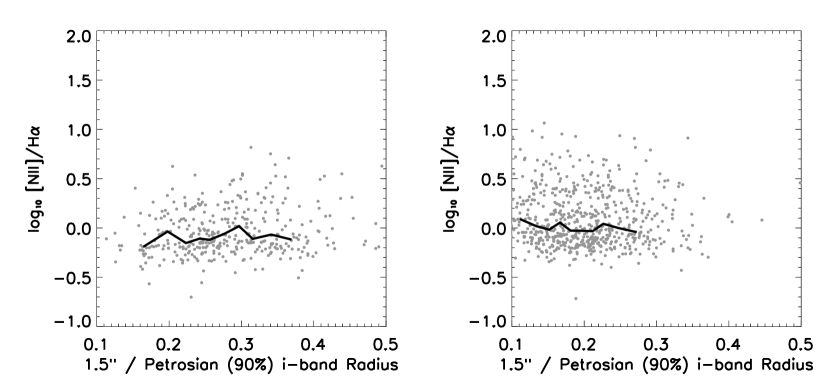
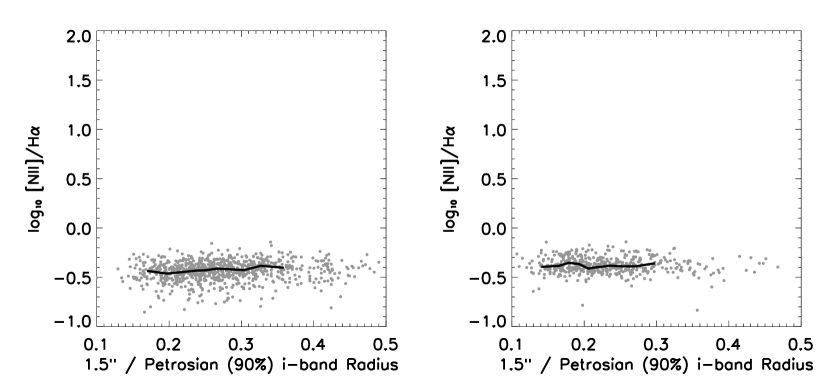
We investigate here aperture effects due to the limited radius of the SDSS spectroscopic fibers (only 1.5 arcseconds in radius), using the SDSS photometric data to measure the fraction of light contained within the fiber (1.5 arcseconds), compared to the total light of a galaxy, as defined by the Petrosian 90% radius (see Stoughton et al. 2001 for more details). We begin by noting that this fraction is approximately the same for all galaxy types discussed herein, i.e., we find the fraction of the total light within the fiber to be 25% for star-forming galaxies, 23% for AGN, and 27% for passive galaxies. Thus, over our redshift range, our spectral identifications are not biased towards any specific galaxy type.

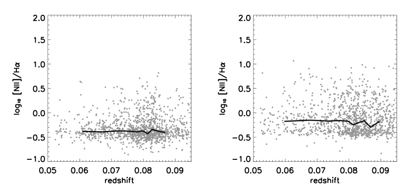
In Figure 6, we plot the measured [NII]/H$\alpha$ line ratio, as a function of the fraction of the total light within the SDSS fiber, for galaxies classified as either an AGN or a star–forming galaxy. We see no evidence for any aperture bias for either AGNs or star-forming samples (nor as a function of luminosity). In Figure 7, we plot the measured [NII]/H$\alpha$ line ratio as a function of redshift and again, see no evidence for aperture bias with redshift.

2.7. Completeness

The main SDSS galaxy sample is designed to be near complete to our chosen magnitude limit (see Strauss et al. 2002) and therefore, we expect our pseudo volume–limited sample of galaxies to be nearly-complete in both redshift and absolute magnitude within the limits specified in Section 2. The use of an absolute magnitude limited survey is crucial for future comparisons to theoretical work (via simulations or semi-analytic techniques). We stress that our AGN fraction as determined using all unambiguous classifications (19% as seen in Table 1) is relatively robust against the chosen magnitude limit for our sample. For instance, the AGN fraction increases only slightly, from 19% to 22%, over the magnitude range $-19\leq M_{r}\leq-22$ respectively. We have difficulty probing magnitudes which are brighter (too few galaxies) or dimmer (the sample becomes very incomplete) than these limits.

It is also worth pointing out that the SDSS has a firm lower limit on the signal-to-noise ratio of any observed spectrum, which alleviates any concerns regarding the homogeneity of identifying emission lines in these spectra. To test this, we measure the mean signal–to–noise ratio for each of the different classification of galaxies in our sample and found that the passive population (no emission lines greater than 2$\sigma$) had the highest mean signal–to–noise of all the sub–samples, i.e., a mean S/N of 27.7 compared to a mean S/N of 23.8 for the AGNs and a mean S/N of 18.5 for the star–forming populations. Therefore, these passive galaxies are truly passive as they possess the required signal–to–noise to detect the expected emission lines seen in AGNs, LLAGNs and star-forming galaxies. The ELU galaxies ($34$% of all galaxies in our sample) have a mean signal–to–noise ratio of 24.8. Therefore, in terms of our galaxy classifications, our total galaxy sample is 66% complete (in classifications), with the remaining third of galaxies being classified as ELU galaxies. We will discuss these ELU galaxies in Section 3.1.

2.8. Data Summary

For two–thirds of our sample, we have a robust classification of an AGN, passive and star–forming galaxy. For example, the two statistical methods used to identify AGNs and star–forming galaxies produce similar fractions. The first method, which is common in the literature, is less conservative than our FDR method, and produces a slightly larger sample of AGNs. However, the differences are marginal, indicating that our galaxy classifications are robust to the method used and the errors on the line measurements. The AGN classifications are thus robust against the exact classification of the transition objects. Therefore, for the remainder of the paper, we use the $>2\sigma$ line method to classify our galaxies to remain consistent with the previous literature.

We have compared our AGN classification to those using template-fitting techniques (e.g., Coziol et al. 1998) and find excellent agreement (see Figure 5). This is due to our “2–line” method of classifying AGNs, which only requires the stronger H$\alpha$  and [NII]  lines. Finally, we have shown that stellar absorption does not strongly affect our classifications and that our classifications are free of any aperture bias. The remaining third of our sample is unclassified and could be affected by measurement error, stellar absorption and classification technique. We make no attempt to individually classify these galaxies, but instead statistically model their distributions (see Section 3.1).

3. AGN Fractions versus Density

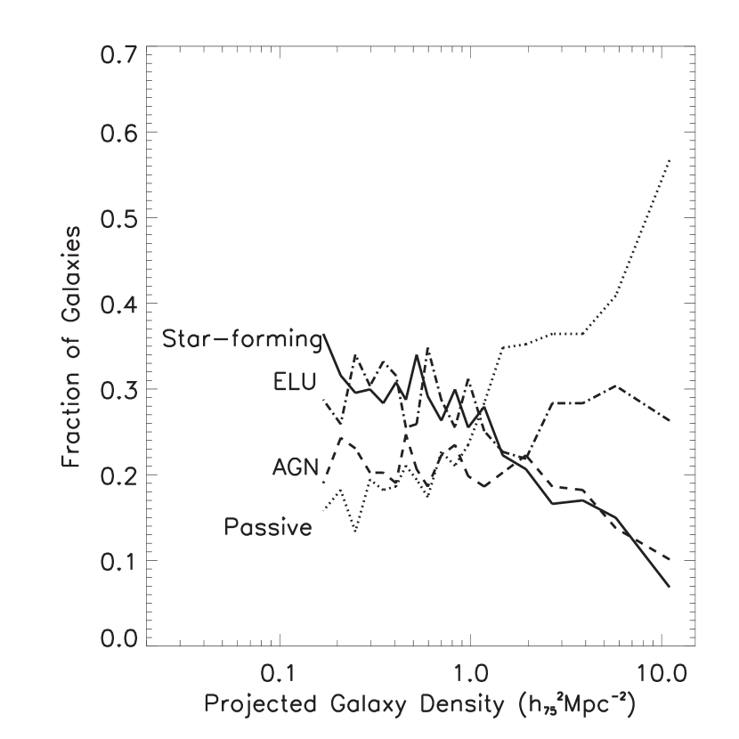
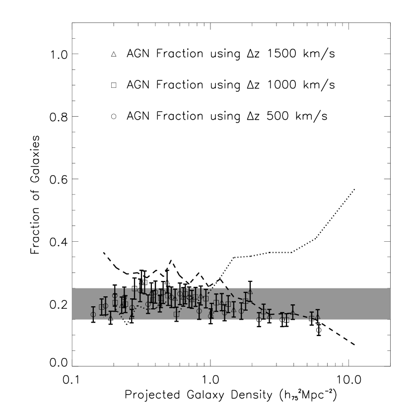
In Figure 8, we plot the fraction of galaxies in each of our classifications (star–forming, passive, AGN, ELU) as a function of the projected local galaxy density, which is identical to that used, and described, in Gomez et al. (2003). Briefly, this projected local galaxy density is determined from the distance to the $10^{th}$ nearest projected neighbor (within our pseudo volume–limited sample) within a redshift shell of $\pm 1000{\rm km\,s^{-1}}$ centered on the central galaxy. We then convert this surface density (within the redshift shell) into a local projected galaxy density. This approach is adaptive as the width of the smoothing kernel changes as a function of the local density and has the advantage, over a fixed width kernel density estimator, of having a constant signal–to–noise for all environments. We show in Figure 9 that our density estimates are robust against choices of the size of the redshift shell and independent of redshift.

Figure 8 shows the expected decrease in the fraction of star–forming galaxies in dense regions and the increase in the fraction of passive galaxies in dense environments. These relations are analagous to SFR–density and morphology–density relations of Gomez et al. (2003) and Dressler et al. (1997) respectively. Figure 8 confirms an earlier analysis by CFGKM who used an entirely different dataset and data-reduction procedure. As in CFGKM, we find that the AGN fraction is constant over the two orders of magnitude in local galaxy density probed by this work, i.e., spanning a density range that includes the cores of rich clusters to the rarefied field population. The small decrease in the AGN fraction in the densest regions is not statistically significant; a line with zero slope is a good fit to the fraction versus density.

In addition, we have performed chi-square tests on the fraction distributions in Figure 8 (Left). In this analyis, we measured the chi-square test statistic using the mean of the fraction per galaxy type as the null hypothesis. This test then tells us whether we can rule out a constant fraction (defined by the mean) as a function of density for each galaxy type. For AGN, we can only rule out a constant AGN fraction at the 46% level (i.e., a constant AGN fraction cannot be ruled out for this data). On the other hand, we can rule out a constant star-forming fraction at the $>$99.9999%  level, and a constant fraction of passive galaxies is ruled out at the 99.999%  level. We have looked at this statistic using only 2–line or 4–line AGNs as defined above and also find that the a mean constant fraction cannot be ruled out for the either of these subsets of AGNs. We can restate this result in that the dip in the inner-most bin of the AGN fraction seen in Figure 8 (Left) is not significant. We note that there are a significant number of ELUs in this bin, which must be classified as either star-forming or AGN. In the next section, we address how the ELU galaxies might contribute to the AGN and star–forming fractions.

3.1. Identifying and Modeling the ELU Galaxies

Unfortunately, in Figure 8, 34% of our galaxy sample remains unclassified as either an AGN or star–forming galaxy; these are the ELU galaxies discussed in Section 2.2 and their fraction as a function of density is shown in Figure 8. These ELU galaxies cannot be passive as, by definition, they contain at least one significantly detected emission line ($>2\sigma$). In this section, we first try and classify as many of these ELU galaxies as possible using the available spectroscopic information. Then, for the remaining ELU galaxies, we statistically model their contribution to the AGN and star–forming fractions seen in Figure 8, using only our current knowledge of the environmental dependence of star–forming galaxies.

3.1.1 Upper Limits on Missing Emission Lines

We discuss here a technique for classifying ELU galaxies based on the combination of detected ($>2\sigma$) emission lines and upper limits on the non–detected emission lines ($<2\sigma$). For example, most of the ELU galaxies in fact have $>2\sigma$ detections of both the H$\alpha$  and [NII]  emission lines, but are missing detections of the weaker H$\beta$  and [OIII]  lines. These galaxies were not classified as AGNs, using the 2–line method discussed in Section 2.2, as their observed [NII]/H$\alpha$  line ratio was below the threshold required for them to be unambiguous 2–line AGN detections (see Section 2.2 where we defined log([NII]/H$\alpha$)$>-0.2$ as the threshold). However, for these ELU galaxies, we can make a reasonable estimate of their classification using the observed upper limits on the fluxes of the [OIII]  and H$\beta$  emission lines. The flux upper limits on these missing lines is taken to be twice the measured flux error on that line, as this is our criteria for considering a line as detected, i.e., $>2\sigma$.

By using a combination of upper limits and detected emission lines, we compute the line ratios for these ELU galaxies and place them on the usual diagnostic diagram (Figure 3). If the ELU galaxies lie below the model in Figure 3, then it is reasonable to assume that these galaxies are star–forming, as the true values for the missing [NII]  and/or [OIII]  emission lines must be smaller than their upper limits, which would move the galaxies further into the star–forming region of Figure 3. We have used this technique to classify a further 230 of 1651 ELU galaxies as star–forming, bringing the fraction of star–formation galaxies in our sample to 26% (up from 21% in Table 1). All of these additional 230 galaxies were not originally classified using the 4–line method because they were missing a detection of the [OIII]  line (which is a good indicator of AGN activity). These 230 star-forming galaxies have a significantly smaller median H($\alpha$) EW of $\simeq 14$, compared to a median H($\alpha$) EW of $\simeq 26$ for the 4–line classified star-forming galaxies, i.e., they have on average lower SFRs.

Likewise, we can classify ELU galaxies using the upper limits on any missing H$\alpha$  and/or H$\beta$emission lines, and detections of the [NII]  and [OIII]  emission lines. In this case, if the observed line ratios for such ELU galaxies place them above the model in Figure 3, then it is reasonable to assume that these ELU galaxies contain an AGN, as the true value of H$\alpha$  and/or H$\beta$  is smaller than the upper limit thus forcing the galaxy further into the AGN region of Figure 3. Using this methodology we classify an additional 40 ELU galaxies as AGNs, bringing the AGN fraction up slightly to 20%. All of these galaxies were previously missed because of weak H$\beta$  emission, which is a good indicator of recent star–formation.

Using these new techniques, based upon the upper limits of missing lines, we have reduced the fraction of ELU galaxies from 34% to 28% of all galaxies in our sample. In the next section, we statistically model the classifications of the remaining ELU galaxies.

3.1.2 Statistical Modeling of ELU Galaxies

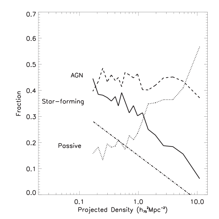
Figure 8 shows that $\sim 30\%$ of galaxies in the densest environments are ELU galaxies. These ELU galaxies are either an AGN or star–forming. It is now well established using complete galaxy samples that the median SFR of galaxies in the cores of clusters is low, and that the fraction of star–forming galaxies is also low (see Gomez et al. 2003; CFGKM). Therefore, it is likely that most of the ELU galaxies in dense environments are AGNs, and not star–forming. Under this assumption, we can statistical model these ELU galaxies and assign most of them in dense regions to our AGN fraction. In creating this model, we first measure the fraction of unambiguous star–forming galaxies over the total number of unambiguous star–forming galaxies plus AGNs, versus density. Since the AGN fraction does not vary with density, the slope of this fraction versus density is identical to the slope of the star–forming fraction versus density (shown in Figure 8). We then fix the amplitude of this relation such that the fraction of star–forming galaxies in the densest regions is $5\%$, which is similar to the fraction seen by CFGKM (in their highest density bin). Our final model, i.e., the fraction of ELU galaxies which are star–forming versus density, is shown as the dash-dot line in Figure 8. We then add this modeled fraction of star–forming and AGN ELU galaxies, as a function of density, to the existing fractions of unambiguously classified star-forming galaxies and AGNs (from Section 2.2 and Figure 8). In Figure 8, we show the final fractions of galaxies which are classified as star–forming, AGN, and passive versus density for our total sample of 4921 galaxies. We note that 82% of the ELU galaxies, which were not classified using the upper limits on the emission lines, were statistically classified as AGNs, while the remainder are star–forming.

3.1.3 Testing our Model

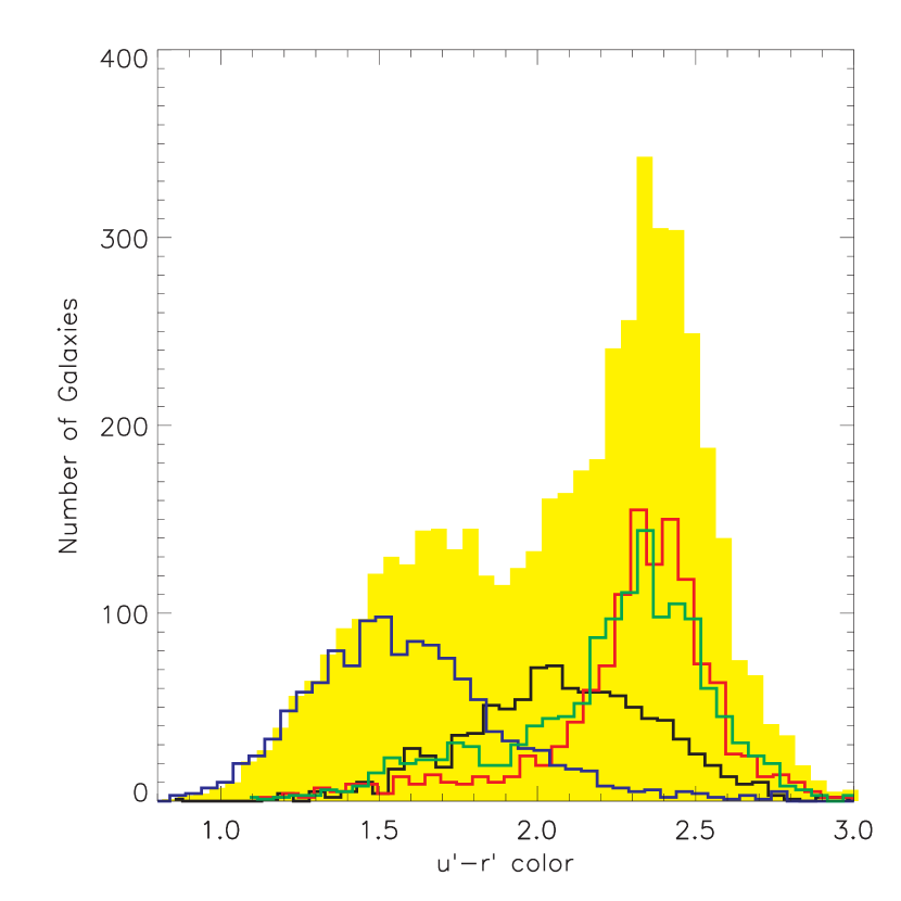
Before we interpret our results, it is fair to question the reliability of our empirical modeling. We test our model using the SDSS photometric imaging data via the colors of our galaxies. In particular, we use the $u^{*}-r^{*}$ rest-frame color as an indicator of on–going star–formation, as the $u$-band flux from these galaxies will be dominated by young, massive stars (see Strateva et al. 2001). The colors also have the advantage of measuring the total spectral energy distribution of the whole galaxy (we use Petrosian magnitudes here) and are therefore, unaffected by fiber aperture effects and stellar absorption problems. In Figure 10, we show the distributions of color (SDSS $u^{*}-r^{*}$) for all galaxies in our sample. The star–forming and passive galaxy populations follow the expected trends, i.e., the star–forming galaxies are the bluest (in $u^{*}-r^{*}$) galaxies in our sample, while the passive galaxies are the reddest. The AGN population lie between these two populations; redder than the star–forming galaxies, but slightly bluer than the passive galaxies.

Figure 10 shows the distribution of color for the ELU galaxies which could not be identified using upper limits on the missing emission line, i.e., the sample of ELU galaxies that we statistically classified. Clearly, the bluer ELU galaxies are likely to be star–forming, while the redder ELU galaxies are likely AGNs as, by definition, their spectra contains at least one significant emission line. As a test of our classification methods, we note that 90% of the 230 ELU galaxies we classified as star–forming using the upper limits in Section 3.1.1 have $u^{\prime}-r^{*}$ colors of $<2.0$, which is fully consistent with the observed colors of our unambiguously classified star-forming galaxies. This is strong confirmation that these ELU galaxies are truly star–forming and the methods we employ are robust.

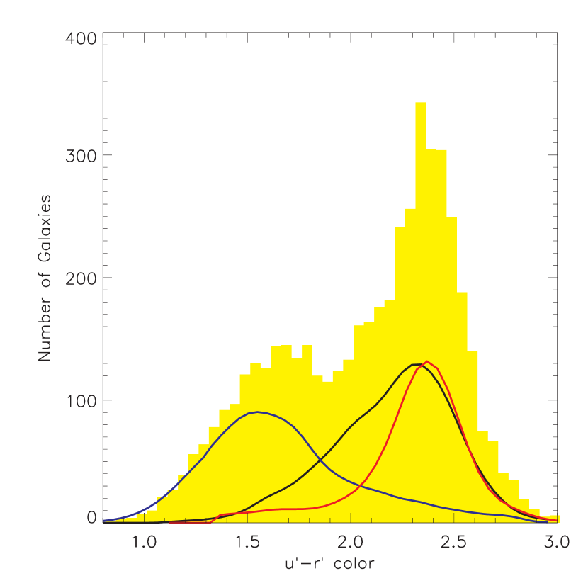
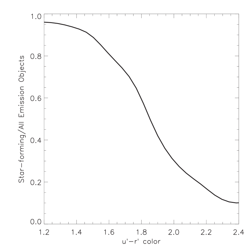
We can also model the distribution of star–forming galaxies and AGNs in the ELU galaxies by assuming that the color distribution for the fraction of unambiguous star–forming galaxies (4–line method) over all unambiguously classified galaxies, is correctly measured in our sample. This fraction is shown in Figure 11 and simply states that nearly all galaxies with $u^{*}-r^{*}<1.5$ are star–forming galaxies, while above $u^{*}-r^{*}>2$, nearly all our unambiguously classified galaxies possess an AGN. We apply this model to the sample and show in Figure 10 (right) the resulting color distributions for our classifications. This model identifies 77% of the ELU galaxies as AGNs, while the remaining 23% are identified as star–forming. These observed fractions, which are based solely on the total colors of these ELU galaxies, are consistent with our model described above.

Finally, we considered here the effects of dust extinction (reddening) on our observed color distributions. For example, dusty star–forming galaxies could mimic the colors of our unambiguously classified AGNs and would cause an over–estimation of the AGN fraction in the ELUs galaxies. To quantify this problem, we use the Bruzual & Charlot (2001) spectral synthesis models to estimate the amount of dust extinction and metalicity required to redden the $u^{*}-r^{*}$ color of a star–forming galaxies such that it would be mis–classified by our methods as an AGN. We begin by calculating the $u^{*}-r^{*}$ color for a $z=0.07$ star–burst galaxy 0.3 Gigayears after its burst and with a dust extinction similar to that of our Galaxy (see Charlot & Longhetti 2001 for these parameters). The predicted $u^{*}-r^{*}$ color of such a galaxy is fully consistent with the observed $u^{*}-r^{*}$ colors of our star–forming galaxies ($u^{*}-r^{*}=1.5$). We then increased the dust extinction, keeping all other parameters fixed, until we obtained the mean $u^{*}-r^{*}$ color observed for our AGNs. We find that we require an additional 4 magnitudes of dust extinction (beyond that seen in our Galaxy) to result in a mis–classification of these star–forming ELU galaxies. This is a large amount of extinction and is unlikely to affect 25% of bright galaxies in the local Universe which are under–going active star–formation. We therefore conclude that it is highly unlikely that star–forming galaxies make up a large portion of the ELU galaxies.

3.2. AGN Fraction as a Function of Galaxy Morphology

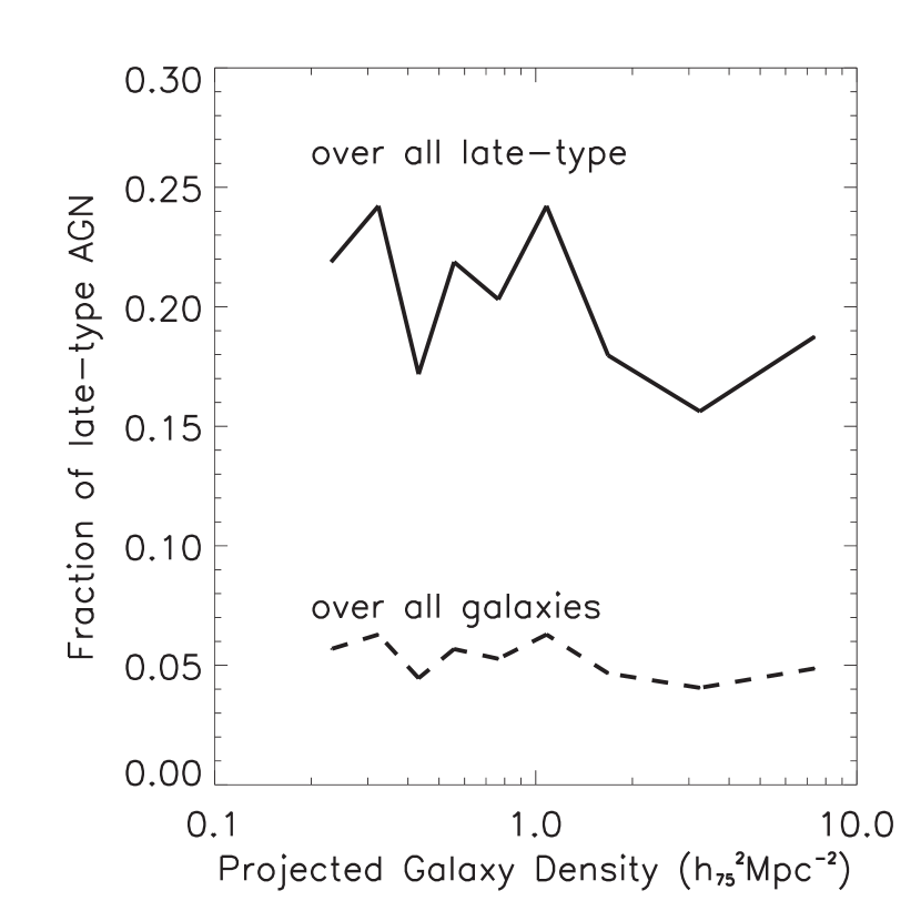
In this section, we study the fraction of AGNs in galaxies as a function of the morphology of the host galaxy. First, we utilize the inverse concentration index ($C_{in}$) in the SDSS $r$ band, which is defined to be $r_{50}/r_{90}$, where $r_{50}$ is Petrosian radius containing 50% of the light and $r_{90}$ is Petrosian radius containing 90% of the light (see Stoughton et al. 2002; Strateva et al. 2001). Therefore, a galaxy with a diffuse light distribution (a spiral galaxy) would have a high concentration index, while compact galaxies have a low index value. As in Gomez et al. (2003), we use a threshold $C_{in}\geq 0.4$ to identify late–type (spiral) galaxies, which is higher than the $C_{in}\geq 0.33$ threshold proposed by Shimasaku et al. (2001) and Strateva et al. (2001). We prefer the higher threshold in $C_{in}$ as it provides a purer, yet more incomplete, sample of spiral galaxies than those advocated by Shimasaku et al. (2001) and Strateva et al. (2001). In Figure 12, we present the AGN fraction for galaxies with $C_{in}\geq 0.4$ (late–type galaxies) as a function of local galaxy density. As seen in Figure 12, we observe no trend with density for just the late–type (spiral) galaxies and the fraction of all late–type galaxies with an AGN is 20%.

To study the fraction of early–type galaxies with an AGN, we can not use $C_{in}<0.4$ as this sample is severely contaminated by late–type galaxies (see Gomez et al. 2003; Shimasaku et al. 2001; Strateva et al. 2001). As an alternative, we can study the subset of galaxies that reside in known clusters of galaxies, as these galaxies will be predominately early–type (ellipticals and S0’s) galaxies. To achieve this goal, we use the C4 cluster catalog which was described in Gomez et al. (2003) and Nichol (2003). In this paper, we use a sample of 23 C4 clusters in the EDR area that have a mean redshift between $0.053\leq z\leq 0.092$. We then select 967 galaxies from our original sample that lie within a projected distance of 2 virial radii from one of these clusters, and within $|z_{galaxy}-z_{cluster}|\leq 4\sigma_{v}$, where $\sigma_{v}$ is the velocity dispersion of the clusters. In Table 1, we provide the fraction of galaxy as a function of our classifications (passive, star–forming and AGN) for these 967 cluster galaxies. As expected, the fraction of star–forming galaxies is lower for these cluster galaxies than for our full sample (see Table 1). As seen in Gomez et al. (2003), the fraction of star–forming galaxies becomes significantly lower in the inner (projected) 500kpc of these 23 clusters. Likewise, the fraction of passive galaxies (no detected emission lines) is higher in clusters than for the full sample, and continues to increase towards the inner (projected) 500kpc of our clusters. However, we again observe that the fraction of galaxies with an AGN remains nearly the same in our 23 clusters as for our full sample, and we only witness a small decrease (which is statistically insignificant) in the fraction of AGNs within the inner (projected) 500kpc of our clusters.

We note that we have not modeled the ELU galaxies in our cluster analysis (as we did in Section 3 for the galaxy densities). However, it is worth noting in Table 1 columns 2 and 3, that there is large number of ELUs in the cores of clusters. As we expect most of these ELUs to be AGNs, a model for cluster ELUs similar to the one used in Section 3.1 would have the same consequences as shown in Figure 8: raising the total fraction of AGNs and keeping the fraction of AGNs constant.

Table 1Galaxy Type Fractions

Galaxy Type	Fraction (all galaxies)	Fraction $<2$ Rvirial	Fraction $<0.5$ Rvirial
	(cluster and field)	(cluster)	(cluster)
AGN	19%	17%	14%
Star–forming	21%	16%	9%
Passive	26%	35%	46%
ELU	34%	32%	32%

3.3. AGN Fraction Summary

In Figure 8, we show the AGN fraction as a function of local galaxy density for our pseudo volume–limited sample of galaxies. In this figure, we present two versions of the AGN–density relation. The left–hand plot represents the absolute lower limit on the AGN fraction, as we only plot our unambiguously classified AGNs and assumes all the unclassified emission line galaxies are star–forming. This is clearly unreasonable. The right–hand plot presents the AGN fraction as a function of local galaxy density when we use our final AGN classifications based on all the methods discussed herein, i.e., both the 4–line and 2–line method, as well as the upper limits and statistical modeling of the ELU galaxies. This is a more realistic representation of the true AGN–density relation. In both cases however, our AGN–density relation is consistent with a constant AGN fraction over two orders of magnitude in local galaxy density.

We have extensively tested our classifications of the ELU galaxies. We find that the fraction of ELU galaxies which contain an AGN is $\sim 75\%$, which is consistent with the model we employed in Figure 8, which is based on the environmental dependence of unambiguous star–forming galaxies (the dotted line) . Therefore, our classifications are robust and internally consistent, i.e., the color, environment and emission lines of these ELU galaxies all point to the same classification. In total, we find that $\simeq 40\%$ of galaxies in our pseudo-volume-limited sample contain an AGN, which is remarkably consistent with the 43% measured by Ho et al. (1997). We note that previous samples have different luminosity limits and selection algorithms and these must be accounted for in any detailed comparison of AGN fractions. Also, we remind the reader that this value of 40% is only valid in the context of the model we apply (i.e. that most ELUs in clusters are not star-forming according to the known star-formation density and star-formation-fraction density relation

4. Discussion

4.1. Comparisons to Previous Works

Based on our sample of unambiguously identified AGN, the overall fraction of galaxies with an AGN we observe (20%) is similar to that reported by CFGKM, who found that 17% of their magnitude limited sample of $\sim$3500 galaxies ($m_{R}\leq 15.4$) possessed an AGN. We note that the AGN classification process used by CFGKM is very similar to ours, while the galaxy samples are nearly independent. Carter et al. (2001) further suggested that as many as 28% of their sample could be AGN, if they classify all of their unclassified emission line galaxies as AGN. By modeling our unclassified emission line galaxies (Section 2.2), we find that $\sim$ 40% of our sample could be AGN. This larger fraction is closer to that found by Ho, Filipenkko & Sargent (1997) who used the Palomar survey of galaxies to identify AGNs.

The fraction of galaxies in our sample that definitely harbor an AGN ($20\%$) is significantly higher than found in the earlier studies of Dressler et al. (1984) and Huchra & Burg (1992). We also find our fraction to be significantly larger than that reported by Ivezic et al. (2002), who found that 5% of SDSS galaxies had an AGN. This could be the result of the different AGN classification techniques, e.g. Ivezic et al. (2002) required at least four $>3\sigma$ detected emission lines for each galaxy, and used a higher threshold for separating AGNs from star–forming galaxies than used here. Interestingly, Ivezic et al. (2002) finds that by only using those SDSS galaxies which have radio match (ignoring their spectral AGN classifications), then the potential AGN fraction rises to 30%, more in agreement with our results. All together, these works suggest that at least $\sim 20\%$ of luminous galaxies have an AGN, but the true fraction is probably closer to $\sim 40\%$. We note that we have not performed a fully detailed comparison of previously measured AGN fractions. Such an analysis would need to take into account the variety of selection differences and the incompleteness in their respective samples.

We find that the fraction of galaxies with an AGN is independent of environment. This result is consistent with the works of Coziol et al. (1998), Shimata et al. (2000), Monaco et al. (1994), and Schmitt (2001), who use a variety of techniques to quantify environment of AGNs. Our results are also in agreement with the recent analysis by CFGKM, who use a similar method for measuring the local galaxy density. We also show that the AGN fraction in clusters is the same as for all galaxies, which is different from Dressler et al. (1984) who find five times as many AGN in the field as in clusters. We attribute this difference to the selection criteria used by Dressler et al., specifically they missed both the [NII]  and $H\alpha$ emission lines (see also Way, Flores, and Quintana 1998).

Our results are also consistent with the recent quasar clustering analyzes of Croom et al. (2002) and Oltram et al. (2002) for the 2dF QSO Redshift Survey (2QZ). These authors find that the clustering of luminous quasars (at a mean redshift of $z=1.4$) is identical to that of local galaxies, thus suggesting that these two populations (galaxies and quasars) where formed about the same time and follow the same density distribution. This conclusion is re–enforced by Cattaneo & Bernardi (2003) who use the stellar ages of SDSS ellipticals to constrain the cosmic accretion history of supermassive black holes. Taken together, these works clearly indicate that AGNs (including quasars) could be unbiased tracers of the galaxy distribution at both low and high redshift. However, the Martini et al. (2002) study of X-ray classified AGN notes that many optical AGN in cluster may be obscured by dust. If this were the case, one could not recover 100% of the AGN population using optical studies alone.

4.2. Physical Interpretation

In Figure 8, we confirm the findings of Gomez et al. (2003) and Lewis et al. (2002) that the SFR–density relation has a “critical density” at $\simeq 1h^{-2}Mpc^{2}$, i.e. below this density the fraction of galaxies that are star–forming is high and constant (see Postman & Geller 1984), while above this density the fraction drops rapidly. Likewise, we see the opposite trend for the passive galaxies (with no emission lines) in that the fraction of such galaxies increases rapidly above the critical density of $\simeq 1h^{-2}Mpc^{2}$, i.e., consistent the morphology–density (Dressler et al. 1997; Postman & Geller 1984). It is therefore surprising that the AGN population has no apparent AGN–density relation, as other properties of galaxies (morphology, luminosity, star–formation rate etc.) show a strong dependence on local galaxy density (Gomez et al. 2003; Hogg et al. 2002). We also find no AGN–density relation for the early– and late–type galaxies.

These observations can be naturally understood under the hypothesis that the AGN population is primarily tracing only the bulge component of galaxies. This hypothesis would explain why we see no dependence on local galaxy density, as most galaxies have a bulge, and why there is no correlation with morphological type, as the disk component is irrelevant to the existence of an AGN. Such a model would then suggest that star–formation in the disk of a galaxy is not driven by the presence of an AGN, and vica versa. This hypothesis is also consistent with the fact that most of our AGNs appear to be redder in their overall $u^{*}-r^{*}$ color) than known star–forming galaxies. If there were a strong relationship between the existence of an AGN and the ability of a galaxy to form stars, we might expect the AGN fraction to decrease with density, as the star-forming fraction is seen to descrease with density.

Our hypothesis is supported by the observations of Ho et al. (1997) and Martini et al. (2002) who see a strong correlation between the properties of AGNs and the bulge of their host galaxies. Furthermore. Kormendy & Gebhardt (2001) observe that the mass of the central supermassive black hole in nearby galaxies is independent of the luminosity of the disk component of a galaxy and only correlates with the properties of the galactic bulge. This hypothesis is also consistent with the idea that AGNs (including quasars) were formed at the same epoch as the old stellar populations in the bulges of these galaxies (Cattaneo & Bernardi 2003).

We should note however, that sub–populations of AGNs are known to be strongly correlated with the morphology of the host galaxy; for example, Seyfert galaxies preferentially reside in spirals and S0s, while radio–loud galaxies are predominantly elliptical galaxies (see Ivezic et al. 2002). Therefore, these sub–populations of AGNs would follow the same density relations as their host galaxies, i.e., the fraction of strongly star-forming galaxies in the cores of clusters is much lower than that seen in the field population. We will investigate such sub–populations of AGNs in our future work; however it is intriguing to note that when the classifications of these sub–populations is ignored (and we simply classify galaxies as AGN or star–forming) the total AGN population becomes independent of local galaxy density. This indicates that the fraction of galaxies classified in these different sub–populations (Seyferts, LINERs etc.) appear to fortuitously sum to a constant over two orders of magnitude in local density.

Our work strongly supports the hypothesis that the bulge of every luminous galaxy, regardless of its overall morphology and environment, contains a supermassive black hole (BH) which is fueling the AGN (see the discussion by Kormendy & Gebhardt 2001). In this model, the black holes, and their mass function, is established at an early cosmological epoch, e.g., through early formation of the galactic bulges in these galaxies (via merger events) and each of these bulges was seeded by BH. This model was recently investigated by Di Matteo et al. (2003) using detailed hydrodynamical simulations to trace the growth and activity of supermassive black holes in galaxies. They found that a majority of the BH mass is accreted by $z\sim 3$ and no further growth happens at later epochs, similar to proposed evolution of galactic bulges. They also found that the BH accretion rate (BHAR) density evolution follows the SFR density evolution to z = 4, but then drops rapidly after that epoch resulting in the BHAR being 100 times lower than the SFR density by $z=1$. Therefore, the BHAR plays no role in the evolution of galaxies at low redshift. In the near future, we should be able to test such predictions using our data from the SDSS.

Under the assumption that every luminous galaxy in our sample contains a supermassive BH, the fraction of galaxies we observe with an AGN ($\simeq 40\%$) must therefore be dependent upon the lifetime (or “duty cycle”) of AGNs (or is dependent on the orientation of the torus surrounding the BH). For example, the interval of look–back time spanned by the redshift range of our sample is $5.7\times 10^{8}$ years (from $z=0.05$ to $z=0.095$). We note that our AGN fraction shows no sign of changing with redshift over this small redshift interval. Therefore, to explain a constant observed AGN fraction of 40%, the average lifetime of these AGNs could be as high as $0.4\times 5.7\times 10^{8}\simeq 2\times 10^{8}$ years. This is longer than previous estimates of the lifetime of an AGN, e.g., a few million years (see Martini et al. 2002), and is longer than the Salpeter lifetime of $4\times 10^{7}$ years (Salpeter 1964). However, it is more consistent with the estimates on the lifetime of quasars from quasar clustering measurements (see Haiman & Hui 2001). One explanation for this longer lifetime is that most of our AGN detections are LLAGNs, where the accretion rate onto the BH is lower than for a normal AGN, thus prolonging the lifetime of the AGN activity.

Alternatively, our AGNs may be experiencing several bursts of activity over the interval of look–back time probed by our sample, i.e., $0.4\times 5.7\times 10^{8}\sim n\,\times\,\tau$, where $\tau$ is the lifetime of the AGN and $n$ are the number of bursts. If we assume $\tau\simeq 10^{7}$ years in agreement with previous observations and the Salpeter time, then this implies $n\sim 40$ bursts between $z=0.05$ and $z=0.095$. In fact, these arguments are simply a re-statement of the fact that we see a high fraction of galaxies with an AGN, so they must be a common phenomenon either because they live a long time, or burst many times. In either case, our observed high fraction of galaxies with an AGN appears inconsistent with a merger–driven model for the fueling of the AGN (Gunn 1979; Kauffmann & Haehnelt 2002), as this would imply a high merger rate for local galaxies. We also see no dependence on environment, which would be expected if AGN activity was primarily driven by galaxy mergers.

5. Conclusions

In this paper, we have studied the fraction of galaxies that possess an AGN as a function of both environment and galaxy type. We have used the Early Data Release of the Sloan Digital Sky Survey to define a pseudo volume–limited sample which is brighter than $M^{\star}+1.45$, within a redshift range of $0.05\leq z\leq 0.95$. Using these data we conclude:

• The overall fraction of galaxies with an AGN is at least $20\%$ (with an unambiguous classification), but maybe as high as $40\%$ if we have correctly modeled the unclassified emission line galaxies in our sample. This confirms the earlier observations by CFGKM and Ho et al. (1997);

• Our results are robust against measurement error on the emission lines, stellar absorption and technique to classify galaxies;

• Over two orders of magnitude, the fraction of galaxies with an AGN is independent of the (projected) local galaxy density (see CFGKM). This is in contrast to star–forming galaxies which are seen to decrease with density (Gomez et al. 2003) and passive galaxies that increase with density (Dressler et al. 1997). Therefore, AGNs are unbiased tracers of the overall galaxy population;

• The AGN fraction is also independent of the overall morphological type of the host galaxy, and therefore, there appears to be no overall relationship between the star–formation activity in the disk component of galaxies and the presence of an AGN. A plausible interpretation of this result is that the AGN phenomenon is related to the bulge component of galaxies, which is consistent with the hypothesis that a supermassive black hole resides in the bulge of all galaxies (see Kormendy & Gebhardt 2001);

• The high fraction of galaxies with an AGN suggests that the lifetime (or “duty–cycle”) of these AGNs is long, or that they burst often. Using the interval in look–back time spanned by our sample, we estimate that the lifetime of AGNs is $\simeq 2\times 10^{8}$ years, which is significantly longer than the Salpeter time. Alternatively, if the lifetime of the AGNs is $10^{7}$ years, then these AGN burst on average $\sim 40$ times between $z=0.095$ and $z=0.05$. If the AGN are merger–driven, then this implies a very high merger rate which is inconsistent with other observations and models.

The authors would like to thank Tiziana Di Matteo, Kathy Romer, Ruper Croft, and Tomo Goto for their help and insightful discussions. AMH acknowledges support provided by the National Aeronautics and Space Administration (NASA) through Hubble Fellowship grant HST-HF-01140.01-A awarded by the Space Telescope Science Institute (STScI).

Funding for the creation and distribution of the SDSS Archive has been provided by the Alfred P. Sloan Foundation, the Participating Institutions, NASA, the National Science Foundation, the U.S. Department of Energy, the Japanese Monbukagakusho, and the Max Planck Society. The SDSS Web site is http://www.sdss.org/.

The SDSS is managed by the Astrophysical Research Consortium (ARC) for the Participating Institutions. The Participating Institutions are the University of Chicago, Fermilab, the Institute for Advanced Study, the Japan Participation Group, The Johns Hopkins University, Los Alamos National Laboratory, the Max-Planck-Institute for Astronomy (MPIA), the Max-Planck-Institute for Astrophysics (MPA), New Mexico State University, the University of Pittsburgh, Princeton University, the United States Naval Observatory, and the University of Washington.

Figure 1.— We present here our analysis of the effect of edge correction on our data set using the mock galaxy catalogs produced by Cole et al. (1999). (Left) We compare here the true distance to the $10^{th}$ nearest neighbor, taken from the mock galaxy catalog without edges, to the measured $10^{th}$ nearest neighbor, taken from a sample of mock galaxies with the same survey geometry as the SDSS EDR. (Right) The same data as shown in the left-hand panel, but now with our edge correction applied as discussed in the text, i.e., we remove all galaxies with an edge closer than the $10^{th}$ nearest neighbor. As one can see, our edge correction removes the biased galaxies in the left-hand panel, but does reduce the dynamic range of densities probed by our analysis, i.e., we are restricted to galaxies with a $10^{th}$ nearest neighbor distance of less than $\sim 6{\rm h_{75}^{-1}}\,{\rm Mpc}$, or a range of densities from $\sim 10{\rm h_{75}^{2}}\,{\rm Mpc^{-2}}$ to $\sim 0.1{\rm h_{75}^{2}}\,{\rm Mpc^{-2}}$.

Figure 2.— We show here the normalised redshift histograms for the whole SDSS EDR catalog (within our absolute magnitude limits; dotted line) and for our sample after edge-corrections (solid-line).

Figure 3.— The line diagnostic diagram traditionally used to differentiate AGNs (red circles) from star–forming galaxies (blue triangles). The solid line is the one–sigma lower limit of the model from Kewley et al. (2001). (Left) The AGNs in this figure are called “4–line AGNs” in the text, as they require all four emission lines to be present for an unambiguous classification. (Right) We plot our classifications using the FDR method described in the text. The FDR method is more conservative and can not classify the “transition objects” (i.e., those galaxies that lie near the model and have a signature of both star–formation and an AGN). However, the two statistical methods used to classify AGNs and star–forming galaxies produce similar fractions.

Figure 4.— This schematic shows how we identify AGNs. The solid curve is the same model used in Figure 3.

Figure 5.— We plot the equivalent width (EW) of the [NII]  emission line versus the line ratio [NII]/H$\alpha$  for galaxies in our sample with $>2\sigma$ detections of these emission lines. The blue triangles are unambiguous star-forming galaxies (4-line method), while the red circles are our 4-line AGN identifications. The green squares are our 2–line AGNs. Many of our 2-line AGNs are normal, i.e., they overlap with the 4-line AGNs, while others are low luminosity AGNs (LLAGNs), delineated using the solid curve. We compare our data to that of the AGNs identified by Coziol et al. (1998) (shown as stars). The solid stars were identified as LLAGNs by Coziol et al. using their template fitting technique, while the open stars are normal AGNs. We find a similar fraction of LLAGNs to normal AGNs in our data as found for Coziol et al. data. We note our data are incomplete for low luminosity star-forming and 4–line AGNs (in the region of log([NII]/H$\alpha$)$<-0.2$ and log(EW(H$\alpha$))$<0.5$) because we require a significant detection of all [NII], [OIII], H$\alpha$  and H$\beta$  emission lines.

Figure 6.— (Top) The observed [NII]/H$\alpha$ line ratio, as a function of the fraction of the total light within the SDSS fibre radius, for galaxies classified as AGNs. The left–hand panel is for dim AGNs, while right–hand panel is for AGN brighter than $M(r)$ = -20.75. The solid line is the median in each bin (with equal numbers of galaxies per bin). (Bottom) Likewise, The observed [NII]/H$\alpha$ line ratio, as a function of the fraction of the total light within the SDSS fibre radius, for galaxies classified as star–forming. The left–hand panel is for dim star–forming galaxies, while right–hand panel is for star–forming galaxies brighter than $M(r)$ = -20.75. The solid line is the median in each bin (with equal numbers of galaxies per bin).

Figure 7.— The same as Figure 6, i.e., the measured [NII]/H$\alpha$ line ratio as a function of redshift for our galaxy sample. (Left) Galaxies less luminous than $M(r)$ = -20.75. (Right) Galaxies more luminous than $M(r)$ = -20.75. The solid line is the median in each bin (with equal numbers of galaxies per bin)

Figure 8.— (Left) The fraction of galaxies as a function of the different classifications (Table 1, column 1), in our pseudo volume-limited sample, as a function density. We see an increase in the fraction of passive galaxies with density, and a decrease in the fraction of star–forming galaxies with density. This is the SFR-density (Gomez et al. 2003) and morphology-density (Dressler 1980; Dressler et al. 1997) relations. The fraction of galaxies possessing an AGN is statistically–consistent with a constant over all local galaxy densities probed here. (Right) We model the AGN/star–forming distribution of ELU galaxies. This model (the dotted line) requires that the overall fraction of star–forming galaxies in dense regions remains small. The resultant AGN and star–forming fractions in this panel include galaxies classified using the upper-limit technique and also the modeled ELUs. The passive fraction remains unchanged.

Figure 9.— (Left) We show the AGN fraction versus local galaxy density using three different redshift shells within which to measure the projected density. The open circles are using $\Delta z$ = 500 km/s, the squares are for $\Delta z$ = 1000 km/s, and the triangles are for $\Delta z=1500$ km/s. (Right) The AGN fraction in three near-equal volume redshift bins. The circles are for $0.05\geq z<0.078$, the triangles are for $0.078\geq z<0.083$ and the squares are for $0.083\geq z<0.095$ (see Gomez et al. 2003). The error bars in this figure are 1/$\sqrt{N}$, where N is the number of galaxies in each bin. The right–hand panel has approximately one–third of the total galaxy sample in each redshift subset, and so there are fewer bins than in the left–hand panel. The dotted-line is the fraction of passive galaxies, while the dashed-line is the fraction of star-forming galaxies. The shaded region encloses an AGN fraction of between 15% and 25% and thus covers the range of AGN fractions discussed in this paper. A straight line (with zero slope) is a good fit to the AGN Fraction data.

Figure 10.— (Left) The distribution of $u^{*}-r^{*}$ color for the different classifications of galaxies used herein. The yellow area is for all 4921 galaxies in our sample. The red line is for passive galaxies. The blue line is for star–forming galaxies. The black line is for unambiguously identified AGN (4–line method), while the green line is for the ELU galaxies. As expected, most passive galaxies are red and most star–forming galaxies are blue. (Right) We now model distribution of color for the AGN and star–forming color distribution of ELUs as in Figure 11. The AGN and star–forming populations now include these ELUs.

Figure 11.— The fraction of unambiguously classified star–forming galaxies over the total number of unambiguously classified galaxies in the sample, as a function of their observed $u^{*}-r^{*}$ color. This demonstrates that most of the blue emission line galaxies are star–forming galaxies, while the red emission line objects are AGN. We use this observed fraction to statistically classify the remaining ELU galaxies.

Figure 12.— The blue line shows the fraction of just late–type (spiral) galaxies that have an AGN. While the red line shows the fraction of all galaxies that are both late–type and have an AGN. This figures shows that late–type galaxies have the same AGN fraction as all galaxies, and there is again no dependence on density.

References

- Baldwin, Phillips, & Terlevich (1981) Baldwin, J. A., Phillips, M. M., & Terlevich, R. 1981, PASP, 93, 5
- Benson, Frenk, & Sharples (2002) Benson, A. J., Frenk, C. S., & Sharples, R. M. 2002, ApJ, 574, 104
- Blanton et al. (2002) Blanton, M. R. et al. 2002, ArXiv Astrophysics e-prints, 5243
- Blanton et al. (2001) Blanton, M. R. et al. 2001, AJ, 121, 2358
- Blanton et al. (2003) Blanton, M.R., Lupton, R.H., Maley, F.M., Young, N., Zehavi, I., & Loveday, J. 2003, AJ, 125, 2276
- Carter et al. (2001) Carter, B. J., Fabricant, D. G., Geller, M. J., Kurtz, M. J., & McLean, B. 2001, ApJ, 559, 606 (CFGKM)
- Cattaneo & Bernardi (2003) Cattaneo, A., & Bernardi, M., 2003, MNRAS, submitted.
- Charlot & Longhetti (2001) Charlot, S. & Longhetti, M. 2001, MNRAS, 323, 887
- Cole, Hatton, Weinberg, & Frenk (1998) Cole, S., Hatton, S., Weinberg, D. H., & Frenk, C. S. 1998, MNRAS, 300, 945
- Colless et al. (2001) Colless, M. et al. 2001, MNRAS, 328, 1039
- Coziol, de Carvalho, Capelato, & Ribeiro (1998) Coziol, R., de Carvalho, R. R., Capelato, H. V., & Ribeiro, A. L. B. 1998, ApJ, 506, 545
- Croom et al. (2002) Croom, S. M., Boyle, B. J., Loaring, N. S., Miller, L., Outram, P. J., Shanks, T., & Smith, R. J. 2002, MNRAS, 335, 459
- Di Matteo, Croft, Springel, & Hernquist (2003) Di Matteo, T., Croft, R. A. C., Springel, V., & Hernquist, L. 2003, Submitted to ApJ, astro-ps/0301586
- Dressler (1980) Dressler, A. 1980, ApJ, 236, 351
- Dressler, Thompson, & Shectman (1985) Dressler, A., Thompson, I. B., & Shectman, S. A. 1985, ApJ, 288, 481
- Dressler et al. (1997) Dressler, A. et al. 1997, ApJ, 490, 577
- Fukugita et al. (1996) Fukugita, M., Ichikawa, T., Gunn, J.E., Doi, M., Shimasaku, K., and Schneider, D.P. 1996, AJ, 111, 1748
- Gómez et al. (2003) Gómez, P. L. et al. 2003, ApJ, 584, 210
- Goto et al. (2003) Goto, T. et al. 2003, ArXiv Astrophysics e-prints, 1305
- Gunn (1979) Gunn, J. E. 1979, Active Galactic Nuclei, Cambridge University Press, 1979, p. 213-225.
- Gunn et al. (1998) Gunn, J.E., et al 1998, AJ, 116, 3040
- Hashimoto, Oemler, Lin, & Tucker (1998) Hashimoto, Y., Oemler, A. J., Lin, H., & Tucker, D. L. 1998, ApJ, 499, 589
- Haiman & Hui (2001) Haiman, Z. & Hui, L. 2001, ApJ, 547, 27
- Ho, Filippenko, & Sargent (1997) Ho, L. C., Filippenko, A. V., & Sargent, W. L. W. 1997, ApJ, 487, 568
- Hogg et al. (2002) Hogg, D. W. et al. 2002, ArXiv Astrophysics e-prints, 12085
- Hogg et al. (2001) Hogg, D.W., Finkbeiner, D.P., Schlegel, D.J., and Gunn, J.E. 2001, AJ, 122, 2129
- Huchra & Burg (1992) Huchra, J. & Burg, R. 1992, ApJ, 393, 90
- Ivezić et al. (2002) Ivezić, Ž. et al. 2002, AJ, 124, 2364
- Kauffmann, Colberg, Diaferio, & White (1999) Kauffmann, G., Colberg, J. M., Diaferio, A., & White, S. D. M. 1999, MNRAS, 303, 188
- Kauffmann & Haehnelt (2002) Kauffmann, G. & Haehnelt, M. G. 2002, MNRAS, 332, 529
- Kewley et al. (2001) Kewley, L. J., Dopita, M. A., Sutherland, R. S., Heisler, C. A., & Trevena, J. 2001, ApJ, 556, 121
- Kormendy & Gebhardt (2001) Kormendy, J. & Gebhardt, K. 2001, AIP Conf. Proc. 586: 20th Texas Symposium on relativistic astrophysics, 363
- Lewis et al. (2002) Lewis, I. et al. 2002, MNRAS, 334, 673
- Loveday, Tresse, & Maddox (1999) Loveday, J., Tresse, L., & Maddox, S. 1999, MNRAS, 310, 281
- Lynden-Bell (1964) Lynden-Bell, D. 1964, ApJ, 139, 1195
- Martini, Regan, Mulchaey, & Pogge (2002) Martini, P., Regan, M. W., Mulchaey, J. S., & Pogge, R. W. 2002, ArXiv Astrophysics e-prints, 12391
- Monaco, Giuricin, Mardirossian, & Mezzetti (1994) Monaco, P., Giuricin, G., Mardirossian, F., & Mezzetti, M. 1994, ApJ, 436, 576
- Miller et al. (2001) Miller, C. J. et al. 2001, AJ, 122, 3492
- Outram et al. (2003) Outram, P. J., Hoyle, F., Shanks, T., Croom, S. M., Boyle, B. J., Miller, L., Smith, R. J., & Myers, A. D. 2003, ArXiv Astrophysics e-prints, 2280
- Pier et al. (2003) Pier, J.R., Munn, J.A., Hindsley, R.B., Hennessy, G.S., Kent, S.M., Lupton, R.H., and Ivezic, Z. 2003, AJ, 125, 1559
- Postman & Geller (1984) Postman, M. & Geller, M. J. 1984, ApJ, 281, 95
- Salpeter (1964) Salpeter, E. E. 1964, ApJ, 140, 796
- Schmitt (2001) Schmitt, H. R. 2001, AJ, 122, 2243
- Shectman et al. (1996) Shectman, S. A., Landy, S. D., Oemler, A., Tucker, D. L., Lin, H., Kirshner, R. P., & Schechter, P. L. 1996, ApJ, 470, 172
- Shimada et al. (2000) Shimada, M., Ohyama, Y., Nishiura, S., Murayama, T., & Taniguchi, Y. 2000, AJ, 119, 2664
- Shimasaku et al. (2001) Shimasaku, K. et al. 2001, AJ, 122, 1238
- Shlosman, Begelman, & Frank (1990) Shlosman, I., Begelman, M. C., & Frank, J. 1990, Nature, 345, 679
- Smith et al. (2002) Smith, J.A., et al 2002, AJ, 123, 2121
- Stoughton et al. (2002) Stoughton, C. et al. 2002, AJ, 123, 485
- Strateva et al. (2001) Strateva, I. et al. 2001, AJ, 122, 1861
- Strauss et al. (2002) Strauss, M.A., et al 2002, AJ, 124, 1810
- Tresse, Maddox, Loveday, & Singleton (1999) Tresse, L., Maddox, S., Loveday, J., & Singleton, C. 1999, MNRAS, 310, 262
- Veilleux & Osterbrock (1987) Veilleux, S. & Osterbrock, D. E. 1987, ApJS, 63, 295
- Way, Flores, & Quintana (1998) Way, M. J., Flores, R. A., & Quintana, H. 1998, ApJ, 502, 134
- Wegner et al. (2001) Wegner, G. et al. 2001, AJ, 122, 2893
- York et al. (2000) York, D. G., Adelman, J., Anderson, J. E., Anderson, S. F., Annis, J., Bahcall, N. A., Bakken, J. A., Barkhouser, R., & the Sloan collaboration. 2000, AJ, 120, 1579