Predicting the Polarization of The Microwave Background from the WMAP Temperature Maps

Abstract

In this paper, we study how to predict the polarization of the Cosmic Microwave Background using knowledge of only the temperature (intensity) and the cross-correlation between temperature and polarization. We derive a “Wiener prediction” method and apply it to the WMAP all-sky CMB temperature maps and to the MAXIMA field.

1 Introduction

Fluctuations in the temperature of the Cosmic Microwave Background (CMB) have been used to map the surface of last scattering for the last decade, since the first results from the DMR instrument on the COBE Satellite (Smoot et al.,, 1992). Now, we have the first results from WMAP (Bennett et al.,, 2003, references therein and elsewhere in this volume) which confirm the CMB anisotropy results gathered over the intervening decade. But the WMAP data promise more than just confirmation: they also offer the first high-sensitivity analysis of the polarization of the CMB (Kogut et al.,, 2003) [although DASI can justly be credited with the first detection of cosmological polarization (Kovac et al.,, 2002)].

The polarized CMB provides independent information on cosmological physics; it traces the flow of the plasma at the surface of last scattering. This flow itself can be decomposed into an irrotational component, corresponding to the action of gravity by the density perturbations responsible for the temperature fluctuations, and a rotational component which can be produced by a background of gravitational waves (e.g., from inflation). These components result in patterns of CMB polarization known, respectively, as “grad” and “curl” (Kamionkowski et al.,, 1997) or, in analogy with electrodynamics, “E” and “B” (Zaldarriaga and Seljak,, 1997). The latter (curl or B) thus has the promise of exploring the physics of the early Universe, but the amplitude of the signal remains well below current detections. Here, then, we concern ourselves with grad or E modes.

However, the WMAP team has yet to produce actual maps of the polarized component of the CMB. Here we investigate a statistical technique to predict the polarization component based on knowledge of the auto- and cross-correlations of the components.

2 Formalism

In this section, we ask the question: if we know the temperature pattern on the sky, as well as the cross-correlation between the temperature and the polarization, what is our best guess at the latter? There are many ways to tackle this question, mathematically if not philosophically equivalent. Here, we take a Bayesian approach, and so start with Bayes’ theorem,

$$P(\theta|DI)=\frac{P(\theta|I)P(D|\theta I)}{P(D|I)}$$ (1)

where $\theta$ labels the parameters we are trying to determine, $D$ the data, and $I$ the background information we are bringing to the problem. $P(a|b)$ is the probability (or probability density) of $a$ given $b$, so $P(\theta|I)$ is the “prior” for $\theta$ and $P(D|\theta I)$ is the likelihood — the probability of getting the specific data $D$ given a fixed set of parameters. The left hand side is the posterior probability, and the denominator just enforces the normalization condition: $P(D|I)=\int d\theta P(\theta|I)P(D|\theta I)$.

How do we apply this to the CMB problem? Let us start with a model for the data, $\Delta_{p}$ as a sum of signal, $s_{p}$ and noise, $n_{p}$,

$$\Delta_{p}=s_{p}+n_{p}\;,$$ (2)

where $\Delta_{p}$ gives the value of the data labeled by $p$, which can include pixel number, frequency of observation, polarization state, etc. We will take the noise to be described by a zero-mean Gaussian distribution with

$$\langle n_{p}\rangle=0;\qquad\langle n_{p}n_{p^{\prime}}\rangle=N_{pp^{\prime}}$$ (3)

where angle brackets are averages over the distribution of the data, and $N_{pp^{\prime}}$ is the noise covariance matrix (which we assume is known, but see Ferreira and Jaffe, (2000); Doré et al., (2001)). We will also take the signal to be a zero-mean Gaussian, with analogous properties to those above, and a signal covariance given by $\langle s_{p}s_{p^{\prime}}\rangle=S_{pp^{\prime}}$.

Thus the actual likelihood function is given by

$$P(\Delta|SN)=\frac{1}{\left|2\pi(S+N)\right|^{1/2}}\exp\left[-\frac{1}{2}\Delta^{\dagger}(S+N)^{-1}\Delta\right]$$ (4)

where we use matrix notation, $\dagger$ refers to the Hermitian conjugate, and vertical bars to the determinant. We can then use Bayes’ theorem to ask for the posterior distribution of any quantity related to the signal, $s_{p}$.

The most obvious quantity we might estimate is the signal itself,

$$P(s|\Delta SN) \propto P(s|SN)P(\Delta|SN)$$ (5)

$$\propto \exp[-\frac{1}{2}s^{\dagger}S^{-1}s-\frac{1}{2}\Delta^{\dagger}(S+N)^{-1}\Delta]$$

$$\propto \exp\left[-\frac{1}{2}\left(s-\langle s|\Delta\rangle\right)^{\dagger}C_{s}^{-1}\left(s-\langle s|\Delta\rangle\right)\right]\;,$$

where the second line comes from assigning a Gaussian prior with variance $S_{pp^{\prime}}$ to the signal, and the final line comes from completing the square, and we have defined

$$\langle s|\Delta\rangle=S(S+N)^{-1}\Delta\qquad\textrm{and}\qquad C_{s}=\langle\delta s\;\delta s^{\dagger}|\Delta\rangle=S-S(S+N)^{-1}S$$ (6)

which give the Wiener filter itself, and the variance about the mean. The Wiener filter has been used in the context of the CMB many times before (e.g., Bunn et al.,, 1996), but primarily as a method of smoothing or for the separation of various foreground components in the signal.

But we can ask a somewhat more general question: what is the distribution of some quantity, $e_{p}$ for which the prior information is that $\langle e_{p}e_{p^{\prime}}\rangle\equiv E_{pp^{\prime}}$ and that it is correlated with the signal, $\langle e_{p}s_{p^{\prime}}\rangle=X_{pp^{\prime}}$? Again, the result is a Gaussian distribution, this time with mean and variance given by

$$\langle e|\Delta\rangle=X(S+N)^{-1}\Delta\qquad\textrm{and}\qquad C_{e}=E-X(S+N)^{-1}X\;$$ (7)

In fact, all of these results can be compressed into two equations, using the notation of Bardeen et al., (1986), already used to some extent above,

$$\langle x|d\rangle = \langle xd^{\dagger}\rangle\langle dd^{\dagger}\rangle^{-1}d\;,\qquad\textrm{and}$$

$$\langle\delta x\;\delta x^{\dagger}|d\rangle = \langle xx^{\dagger}\rangle-\langle xd^{\dagger}\rangle\langle dd^{\dagger}\rangle^{-1}\langle dx^{\dagger}\rangle\;,$$ (8)

where $d=s+n$ and $x$ is correlated with $s$, so $\langle xd^{\dagger}\rangle=\langle xs^{\dagger}\rangle$, which is the cross-correlation, $X$, above. If $x=s$, this reduces the original Wiener filter, Eq. 6, above.

Information about the variance of the Wiener filter is crucial. The Wiener mean itself, $\langle x|d\rangle$, is over-smoothed—low in regimes of low signal-to-noise ratio. A more “typical” signal value is provided by an actual realization from the full posterior distribution: the mean plus a realization of the correlation matrix.

3 Applications

3.1 Full-sky maps

The action of the Wiener filter prediction is clearest when we consider its action on an all-sky map with uniform (or axisymmetric) noise. We start with a noisy temperature map, which we transform into its spherical harmonic components, $d_{\ell m}=a_{\ell m}+n_{\ell m}$, where $a_{\ell m}$ gives the CMB signal and $n_{\ell m}$ the noise. The Wiener filter and variance are given by

$$\langle a_{\ell m}|d_{\ell m}\rangle = \frac{C_{\ell}}{B_{\ell}^{2}C_{\ell}+N_{\ell}}d_{\ell m}$$

$$\langle E_{\ell m}|d_{\ell m}\rangle = \frac{C_{\ell}^{TE}}{B_{\ell}^{2}C_{\ell}+N_{\ell}}d_{\ell m}$$

$$\langle\delta a_{\ell m}\delta a_{\ell m}|d_{\ell m}\rangle = C_{\ell}-\frac{\left(C_{\ell}\right)^{2}}{B_{\ell}^{2}C_{\ell}+N_{\ell}}$$

$$\langle\delta E_{\ell m}\delta E_{\ell m}|d_{\ell m}\rangle = C^{EE}_{\ell}-\frac{\left(C_{\ell}^{TE}\right)^{2}}{B_{\ell}^{2}C_{\ell}+N_{\ell}}$$

$$\langle\delta a_{\ell m}\delta E_{\ell m}|d_{\ell m}\rangle = C^{TE}_{\ell}-\frac{C_{\ell}^{EE}C_{\ell}}{B_{\ell}^{2}C_{\ell}+N_{\ell}}\;,$$ (9)

where we have introduced the experimental beam, $B_{\ell}$, the temperature power spectrum, $C_{\ell}=\langle|a_{\ell m}|^{2}\rangle$, the E-mode polarization power spectrum, $C^{E}_{\ell}=\langle|E_{\ell m}|^{2}\rangle$ and the E-mode polarization/temperature cross power spectrum, $C_{\ell}^{TE}=\langle a^{*}_{\ell m}E_{\ell m}\rangle$. These power spectra are diagonal in $\ell$, and we impose a similar constraint on the noise power, which we denote $N_{\ell}=\langle|n_{\ell m}|^{2}\rangle$. Note that this is an unphysical condition, corresponding to isotropic noise over the sky; if we restrict ourselves to high signal-to-noise experiments and large scales. In these equations, we show the Wiener filter for the temperature itself and for the polarization, and, by extension of the equations from the previous section, the covariance between the two.

We note in passing that the formalism also correctly accounts for the statistics of the polarization “B-modes”. Since the cross-spectrum $C_{\ell}^{TB}=0$, we just have $\langle a^{B}_{\ell m}|d_{\ell m}\rangle=0$ with $\langle\delta B_{\ell m}\delta B_{\ell m}|d_{\ell m}\rangle=C_{\ell}^{B}$ — the data give no new information about them.

We show these formulae for the Wiener filter of the multipole coefficients themselves, but in fact we will always want to smooth the resulting map with some beam (although it is not necessary to use the same as the original experimental beam, $B_{\ell}$).

We can apply these formulae directly to the temperature data from the WMAP satellite. Our requirement of isotropic noise should be adequate for $\ell<400$ where the noise is negligible. In fact, in the following we use the Wiener-filtered temperature maps provided by Tegmark et al., (2003). Note that starting from the temperature Wiener filter enables a slight simplification:

$$\langle E_{\ell m}|d_{\ell m}\rangle=\frac{C_{\ell}^{TE}}{C_{\ell}}\langle a_{\ell m}|d_{\ell m}\rangle\;.$$ (10)

Starting from these Wiener-filtered data, which are in fact available in pixel space, we apply these formulae by going back and forth between pixels and multipole coefficients by performing a spherical-harmonic transform using routines from the HEALPix package (Gorski et al.,, 1999). In Figure 1 we show the Wiener-filtered map of the WMAP data, with the polarization superposed on the temperature.

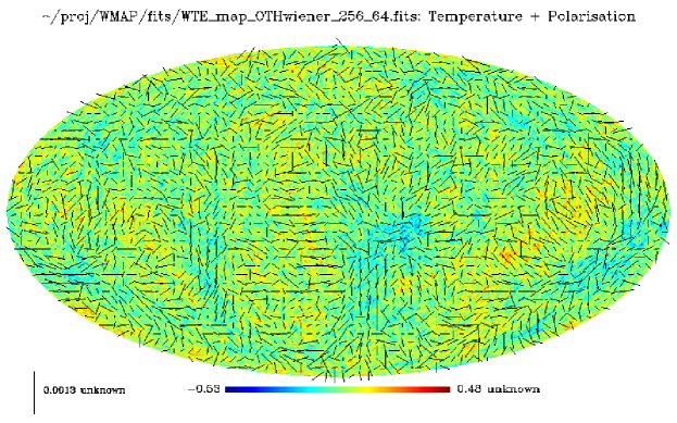
Figure 1: Wiener-filtered map of the CMB temperature and polarization using the WMAP data as prepared by Tegmark et al., (2003).

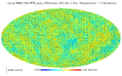
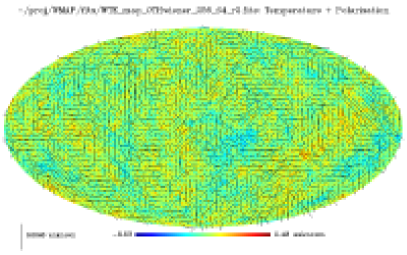
Figure 2: Two realizations of the map of the CMB temperature and polarization using the Wiener-filtered map Figure 1.

In Figure 2 we show 4 realizations of the temperature and polarization drawn from the variances of Eq. 3.1. It is evident that, in fact, the polarization field contains a large uncorrelated component. We can understand this by examining the correlation coefficient,

$$r_{\ell}^{2}=\frac{(C_{\ell}^{TE})^{2}}{C_{\ell}^{E}C_{\ell}}\;.$$ (11)

This correlation coefficient gives the fraction of the power at a given multipole that is correlated between the E-mode polarization and the temperature. In the signal-dominated regime (here, low $\ell$) this gives the correlated fraction of the power in the Wiener filter, as well. In addition, the quantity $1-r_{\ell}^{2}$ gives the fractional amplitude of the variance of the Wiener filter. Thus, if $r_{\ell}\sim 1$, a realization of the Wiener variance is small compared to the Wiener mean, and the mean is a good indication of the actual signal, but if $r_{\ell}$ is closer to $0$, different realizations can look very dissimilar. We plot the correlation coefficient in Figure 3. We see that the correlated fraction depends strongly on $\ell$ (and indeed drops to zero where $C_{\ell}^{TE}=0$) and is everywhere less than about 0.8. In practice, this means that the realizations do vary considerably, but this can in principle be ameliorated by careful filtering of the map to remove those modes where $C_{\ell}^{TE}\simeq 0$.

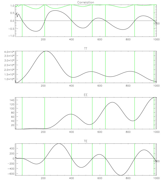
Figure 3: Top Panel: the correlation coefficient, $r$, between temperature and E-mode CMB Fluctuations (bottom curve); the top curve shows $1-r^{2}$. The bottom three panels show the individual power spectra, $C_{\ell}^{XY}$. The vertical lines give the locations where $C_{\ell}^{TE}=0$. Note that the model we use here has optical depth, $\tau=0.17$, responsible for the upturn in the spectra and correlation at low $\ell$.

3.2 Small areas

We can also use the same technique to predict the polarization for small areas of sky, where the available data may be more complicated than that from WMAP. In Figure 4 we show a prediction of the polarization for the field probed by the MAXIMA experiment (e.g., Lee et al.,, 2001). Here, we take the full noise and signal covariance into account, and perform the calculation in pixel space. Instead of performing the calculation $\ell$-by-$\ell$, we must now perform full matrix operations. For the isotropic CMB temperature field with power spectrum $C_{\ell}$,

$$S_{pp^{\prime}}=\sum_{\ell}\frac{2\ell+1}{4\pi}C_{\ell}B^{2}_{\ell}P_{\ell}(\cos\theta_{pp^{\prime}})$$ (12)

where $B_{\ell}$ gives the spherical harmonic transform of the experimental beam and $\theta_{pp^{\prime}}$ is the angle between pixels $p$ and $p^{\prime}$. Analogous formulae hold for the covariances of the polarization components, and slightly more complicated ones for the cross-correlations amongst and between different polarization and temperature components.

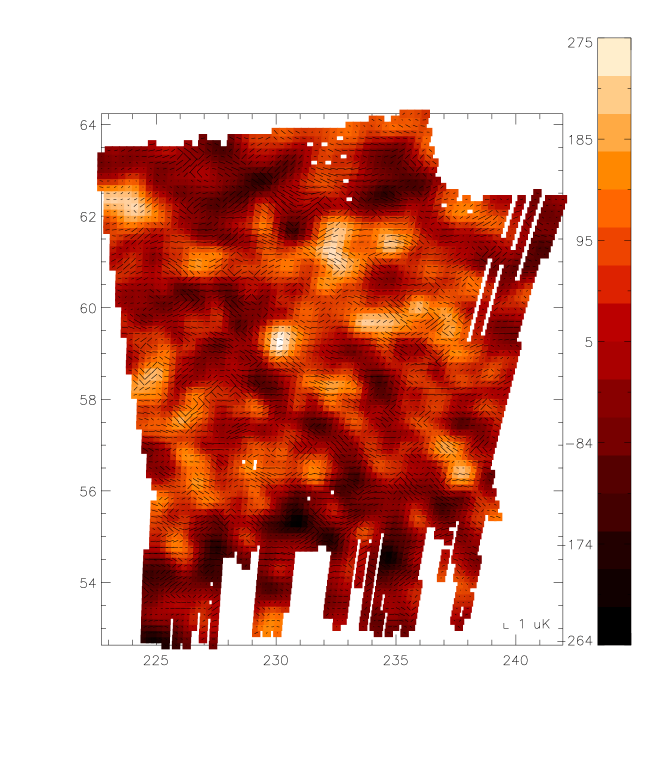
Figure 4: Wiener predicted polarization for the MAXIMA-1 field.

4 Discussion

As mentioned above, the correlation coefficient, $r_{\ell}$ gives an indication of the degree to which the the polarization signal is completely predicted by the temperature signal (and the power spectra $C_{\ell}^{XX^{\prime}}$). The fact that $|r_{\ell}|<0.8$ is an indication that a significant fraction of the E-mode polarization signal is not correlated with the temperature. This leads, finally, to a question about the physics of the temperature-polarization correlations: the correlated component of the polarization and temperature is due in large part to correlations between density and velocity perturbations on the surface of last scattering (Kamionkowski et al.,, 1997; Zaldarriaga and Seljak,, 1997; Jaffe et al.,, 2000; Hu and Dodelson,, 2002). Having only temperature data as discussed here means that the results assume such a relationship between the two components. However, with the availability of actual polarization maps, we should be able to use only minimal theoretical input and yet still recover a two-dimensional snapshot of the plasma flow on the surface of last scattering. We leave the details of this to a future work and, we hope, future data.

Acknowledgments

I would like to acknowledge discussions on this subject with Rob Crittenden, Lloyd Knox and Dick Bond as well as the COMBAT team at Berkeley and elsewhere. My involvement with the MAXIMA team has been invaluable to this work, and in particular has lead directly to Figure 4. This work has been supported by PPARC in the UK.

References

- Bardeen et al., (1986) Bardeen, J. M., Bond, J. R., Kaiser, N., and Szalay, A. S. (1986). The statistics of peaks of Gaussian random fields. Astrophys. J., 304:15–61.
- Bennett et al., (2003) Bennett, C. L., Halpern, M., Hinshaw, G., Jarosik, N., Kogut, A., Limon, M., Meyer, S. S., Page, L., Spergel, D. N., Tucker, G. S., Wollack, E., Wright, E. L., Barnes, C., Greason, M. R., Hill, R. S., Komatsu, E., Nolta, M. R., Odegard, N., Peirs, H. V., Verde, L., and Weiland, J. L. (2003). First Year Wilkinson Microwave Anisotropy Probe (WMAP) Observations: Preliminary Maps and Basic Results. ArXiv Astrophysics e-prints, astro-ph/0302207.
- Bunn et al., (1996) Bunn, E. F., Hoffman, Y., and Silk, J. (1996). The Wiener-filtered COBE DMR Data and Predictions for the Tenerife Experiment. Astrophys. J., 464:1–+.
- Doré et al., (2001) Doré, O., Teyssier, R., Bouchet, F. R., Vibert, D., and Prunet, S. (2001). MAPCUMBA: A fast iterative multi-grid map-making algorithm for CMB experiments. Astron. Astrophys., 374:358–370.
- Ferreira and Jaffe, (2000) Ferreira, P. G. and Jaffe, A. H. (2000). Simultaneous estimation of noise and signal in cosmic microwave background experiments. Mon. Not. R. Astr. Soc., 312:89–102.
- Gorski et al., (1999) Gorski, K., Hivon, E., and Wandelt, B. (1999). Analysis Issues for Large CMB Data Sets. In Banday, A., Sheth, R., and Da Costa, L., editors, Proceedings of the MPA/ESO Cosmology Conference ”Evolution of Large-Scale Structure, pages 37–42. PrintPartners Ipskamp, astro-ph/9812350.
- Hu and Dodelson, (2002) Hu, W. and Dodelson, S. (2002). Cosmic Microwave Background Anisotropies. ARA&A, 40:171–216.
- Jaffe et al., (2000) Jaffe, A. H., Kamionkowski, M., and Wang, L. (2000). Polarization pursuers’ guide. Phys. Rev. D, 61:1462d+.
- Kamionkowski et al., (1997) Kamionkowski, M., Kosowsky, A., and Stebbins, A. (1997). Statistics of cosmic microwave background polarization. Phys. Rev. D, 55:7368–7388.
- Kogut et al., (2003) Kogut, A., Spergel, D. N., Barnes, C., Bennett, C. L., Halpern, M., Hinshaw, G., Jarosik, N., Limon, M., Meyer, S. S., Page, L., Tucker, G., Wollack, E., and Wright, E. L. (2003). Wilkinson Microwave Anisotropy Probe (WMAP) First Year Observations: TE Polarization. ArXiv Astrophysics e-prints, pages 2213–+.
- Kovac et al., (2002) Kovac, J. M., Leitch, E. M., Pryke, C., Carlstrom, J. E., Halverson, N. W., and Holzapfel, W. L. (2002). Detection of polarization in the cosmic microwave background using DASI. Nature, 420:772–787.
- Lee et al., (2001) Lee, A. T., Ade, P., Balbi, A., Bock, J., Borrill, J., Boscaleri, A., de Bernardis, P., Ferreira, P. G., Hanany, S., Hristov, V. V., Jaffe, A. H., Mauskopf, P. D., Netterfield, C. B., Pascale, E., Rabii, B., Richards, P. L., Smoot, G. F., Stompor, R., Winant, C. D., and Wu, J. H. P. (2001). A High Spatial Resolution Analysis of the MAXIMA-1 Cosmic Microwave Background Anisotropy Data. Astrophys. J. Lett., 561:L1–L5.
- Smoot et al., (1992) Smoot, G. F., Bennett, C. L., Kogut, A., Wright, E. L., Aymon, J., Boggess, N. W., Cheng, E. S., de Amici, G., Gulkis, S., Hauser, M. G., Hinshaw, G., Jackson, P. D., Janssen, M., Kaita, E., Kelsall, T., Keegstra, P., Lineweaver, C., Loewenstein, K., Lubin, P., Mather, J., Meyer, S. S., Moseley, S. H., Murdock, T., Rokke, L., Silverberg, R. F., Tenorio, L., Weiss, R., and Wilkinson, D. T. (1992). Structure in the COBE differential microwave radiometer first-year maps. Astrophys. J. Lett., 396:L1–L5.
- Tegmark et al., (2003) Tegmark, M., de Oliveira-Costa, A., and Hamilton, A. (2003). A high resolution foreground cleaned CMB map from WMAP. ArXiv Astrophysics e-prints, astro-ph/0302496.
- Zaldarriaga and Seljak, (1997) Zaldarriaga, M. and Seljak, U. . (1997). All-sky analysis of polarization in the microwave background. Phys. Rev. D, 55:1830–1840.