CRASH: a Radiative Transfer Scheme

Abstract

We present a largely improved version of CRASH, a 3-D radiative transfer code that treats the effects of ionizing radiation propagating through a given inhomogeneous H/He cosmological density field, on the physical conditions of the gas. The code, based on a Monte Carlo technique, self-consistently calculates the time evolution of gas temperature and ionization fractions due to an arbitrary number of point/extended sources and/or diffuse background radiation with given spectra. In addition, the effects of diffuse ionizing radiation following recombinations of ionized atoms have been included. After a complete description of the numerical scheme, to demonstrate the performances, accuracy, convergency and robustness of the code we present four different test cases designed to investigate specific aspects of radiative transfer: (i) pure hydrogen isothermal Strömgren sphere ; (ii) realistic Strömgren spheres; (iii) multiple overlapping point sources, and (iv) shadowing of background radiation by an intervening optically thick layer. When possible, detailed quantitative comparison of the results against either analytical solutions or 1-D standard photoionization codes has been made showing a good level of agreement. For more complicated tests the code yields physically plausible results, which could be eventually checked only by comparison with other similar codes. Finally, we briefly discuss future possible developments and cosmological applications of the code.

1 Introduction

Stimulated by the growing number of observations of the high-redshift universe (e.g. Fan et al. 2001, 2003; Hu et al. 2002), an increasing attention has been dedicated to the theoretical modeling of the reionization process, adopting both semi-analytic and numerical approaches (e.g. Gnedin & Ostriker 1997; Haiman & Loeb 1997; Valageas & Silk 1999; Ciardi et al. 2000, CFGJ; Miralda-Escudé, Haehnelt & Rees 2000; Chiu & Ostriker 2000; Gnedin 2000; Benson et al. 2001; Razoumov et al. 2002; Ciardi, Stoehr & White 2003, CSW). An important refinement has been introduced by the proper treatment of a number of feedback effects ranging from the mechanical energy injection to the H₂ photodissociating radiation produced by massive stars (CFGJ). Only recently, though, the reionization process has been studied in a cosmological context including structure evolution, a realistic galaxy population and a sufficiently accurate treatment of the Radiative Transfer (RT) of ionizing photons through the InterGalactic Medium (IGM), in a simulation volume large enough to have properties “representative” of the all universe (CSW). The next challenge for this kind of study is to develop accurate and fast radiative transfer schemes that can be then implemented in cosmological simulations.

Although the reionization process is one of the most demanding and natural applications of the radiative transfer theory, numerous physical problems require a detailed understanding of the propagation of photons into different environments, ranging from intergalactic and interstellar medium to stellar or planetary atmospheres. The full solution of the seven dimension RT equation (three spatial coordinates, two angles, frequency and time) is still well beyond our computational capabilities and, although in some specific cases it is possible to reduce its dimensionality, for more general problems no spatial symmetry can be invoked. Thus, an increasing effort has been devoted to the development of radiative transfer codes based on a variety of approaches and approximations (e.g. Umemura, Nakamoto & Susa 1999; Razoumov & Scott 1999; Abel, Norman & Madau 1999; Gnedin 2000; Ciardi et al. 2001, CFMR; Gnedin & Abel 2001; Cen 2002). In the following, we give a list of the available cosmological radiative transfer codes, together with their characteristics and applications.

• Gnedin & Ostriker (1997): time-dependent code based on the local optical depth approximation. It solves the evolution of H, He, H₂ and temperature. It includes the RT of radiation from multiple point sources, a background flux and the diffuse component due to recombination. The code is fast, independent on the number of sources, but the approximation breaks down for optical depths of the order of one and cannot account for shadowing effects. It has been applied to the study of the reionization process and has been coupled with hydrodynamical simulations in the implementation of Gnedin (2000).

• Umemura, Nakamoto & Susa (1999): time-independent code based on the method of the short characteristics. It calculates the equilibrium configuration of an isothermal H/He gas. It includes the RT of a background flux and the diffuse component due to recombination. As a backdraw the code can calculate only equilibrium configurations. It has been applied to the study of cosmological reionization.

• Abel, Norman & Madau (1999): time-dependent ray-tracing code. It solves the evolution of hydrogen and treats RT of the radiation emitted by a point source, together with the diffuse component. Although the ray-tracing approach is very accurate, its primary limitation is the high computational cost required to follow a large number of sources and to assure the correct coverage of the simulation volume. This code has been applied to the study of the evolution of the ionized region surrounding a mini-quasar in a cosmological density field.

• Razoumov & Scott (1999): time-dependent ray-tracing code, based on the solution of the 5D (three spatial coordinates and two angles) advection equation. It includes the H, He and H₂ chemistry and the temperature evolution. It treats the RT of radiation from multiple point sources, a background flux and the diffuse component. The code suffers from the same problem as the previous one. It has been applied to the study of the reionization process.

• Ciardi et al. (2001): CRASH 1.0 time-dependent code, based on a Monte Carlo approach. It includes the evolution of an isothermal H gas and it treats the RT of the radiation emitted by point sources, together with the diffuse component. The code has been applied to the study of the evolution of the ionized region surrounding point sources embedded in a cosmological density field.

• Gnedin & Abel (2001): time-dependent code, based on the explicit moment solver OTVET (Optically Thin Variable Eddington Tensor formalism). It includes the H and He chemistry and the temperature evolution. It treats the radiation produced by point sources, a background flux and the diffuse component. Its main problem is related to the correct evaluation of the Eddington tensors. In fact, while the assumption of optically thin Eddington tensor is exact in the limit of a single point source, it may break down in complex situations with very inhomogeneous source functions and opacity fields. It has been coupled with a hydrodynamical simulation to study cosmological reionization.

• Sokasian, Abel & Hernquist (2001): time-dependent ray-tracing code. It includes the H and He chemistry and the temperature evolution. It treats the radiation produced by point sources, a background field and the diffuse component. As a first application, it has been used to the compute HeII reionization by quasars.

• Cen (2002): time-dependent ray-tracing code, based on the fast Fourier transform method for hydrogen ionization. It treats the radiation produced by point sources, a background field and the diffuse component. Unlike conventional ray-tracing schemes where angular discretization is performed on the source, here it is done at the receiving site, guaranteeing good space coverage regardless of the finesse of the angular discretization. Moreover, its speed is independent on the number of sources. The code has been applied to test cases of single and multiple sources embedded in a constant or inhomogeneous density field.

• Razoumov et al. (2002): time-dependent ray-tracing code. It includes the H, He and H₂ chemistry and the temperature evolution. It treats the radiation produced by point sources, a background field and the diffuse component. To alleviate the speed problem related to the ray-tracing approach, the authors have implemented the method developed by Abel & Wandelt (2002), introducing trees of rays segments which recursively split into sub-segment as one moves away from the source. The code has been applied to the study of the reionization process.

Monte Carlo (MC) methods, on which we base our approach, have been widely used in several (astro-)physical areas to tackle RT problems (for a reference book see Cashwell & Everett 1959) and they have been shown to result in fast and accurate schemes. Here we build up on previous work (Bianchi, Ferrara & Giovanardi 1996; Ferrara et al. 1996; Ferrara et al. 1999; Bianchi et al. 2000) to develop a new version of the code CRASH (Cosmological Radiative transfer Scheme for Hydrodynamics), which improves in many ways the earlier version presented in CFMR. The main aim of this paper is to give a full description of the code CRASH in its present form, perform a number of stringent tests that demonstrate its ability to treat RT problems arising in a wide range of astrophysical context, and evaluate its performances. In forthcoming work, we will apply the code to specific cosmological problems.

The plan of the paper is as follows. In Sec. 2 we describe the details of the numerical implementation concerning the discretization of the radiation field and its (time-dependent) interaction with the surrounding matter; we pay special attention to issues as the dependence of spatial and time resolution on the numerical parameters. In Sec. 3, we present results from a set of specifically designed test-runs: Strömgren spheres, two point sources and an optically thick slab case illuminated by a background field. Finally, in Sec. 4, we draw our conclusions and discuss some of the possible future applications and developments of CRASH .

2 Description of the Code

CRASH , is a 3-D numerical code primarily developed to study time-dependent radiative transfer problems in cosmology; however, the versatility of its scheme allows easy extensions to additional astrophysical applications. Such a scheme is largely based on MC techniques, which are used to sample appropriate Probability Distribution Functions (PDFs), as briefly explained in Appendix A. The current version of the code (CRASH 2.0) is a development of a previous implementation of the same scheme, discussed in CFMR. The main differences with that first attempt are [i] the inclusion of helium in all its ionization states, [ii] the self-consistent calculation of gas temperature, and [iii] an efficient algorithm to treat multiple radiation sources and/or a diffuse background field. In addition, more refined photon propagation schemes (see below) have been included. As today, CRASH works as a stand-alone routine that can be applied to arbitrary and pre-computed hydrodynamical density fields. A future development will consist of a full coupling with available cosmological hydrodynamical codes, so that the interaction of radiative transfer and gas dynamics can be treated self-consistently. We now turn to the description of the implementation of the physical processes and the numerical algorithms used by the code.

2.1 Initial Conditions

As a first step, the initial conditions for the physical quantities (gas density, temperature, H and He ionization fractions) must be assigned on the $N_{c}^{3}$ nodes of the adopted 3-D cartesian grid. The density field, the temperature and the ionization fractions can be either the output of a hydrodynamical simulation or arbitrarily constructed. While the density field remains constant during the simulation, i.e. no back-reaction of gas dynamics to the effects of the radiative transfer is considered, the temperature and ionization fractions are instead updated with time. Both open and periodic boundary conditions can be adopted. In the latter case, the ionizing radiation that exits with a given direction from a cell $(x_{b},y_{b},z_{b})$ on the boundary surface of the simulation box, is re-emitted with the same direction from the cell $(-x_{b},-y_{b},-z_{b})$; the origin of the cartesian coordinate system is located at the box center.

Finally, the properties of the radiation field must be specified. The quantities required are the number, location and emission properties (e.g. the intensity of the emitted radiation and its spectral energy distribution) of point sources in the simulated volume, and the intensity and spectral energy distribution of the background radiation, if present. As CRASH has been specifically designed to follow the propagation of ionizing photons, the above spectral parameters are required only for energies $\geq 1$ Ryd. The required properties of the radiation fields are described in detail in the next Section.

2.2 Ionizing Radiation Field

The MC approach to radiative transfer requires that the radiation field is discretized into photon packets; the properties of the radiation field and the relevant radiation-matter interaction processes are then statistically treated by randomly sampling appropriate PDFs. In this approach the ionizing radiation emitted by either a specified number of point sources located arbitrarily in the box, or a background radiation, is easily reproduced. Also, diffuse radiation from recombinations in the ionized gas can be treated in a similar manner without further assumptions.

2.2.1 Point Sources

Let us first consider the case of a single point source with a time-dependent bolometric luminosity $L_{s}(t)$. If $t_{s}$ is the (physical) simulation time, the total energy emitted by the source is:

$$E_{s}=\int_{0}^{t_{s}}L_{s}(t)dt.$$ (1)

Such energy is distributed into $N_{p}$ photon packets, emitted at the source location at regularly spaced time intervals $dt=t_{s}/N_{p}$. Thus, the time resolution of a given run is fixed by $N_{p}$. To each emitted photon packet a frequency, $\nu$, and a propagation direction, $(\theta,\phi)$, are assigned by sampling the source spectrum, $S_{\nu}$, and the angular PDF, using the MC method described in Appendix A. This procedure allows to treat any given spectrum and possible emission anisotropies. The $j$-th monochromatic packet of frequency $\nu$ is then emitted at time $t_{j}=jdt$ ($j=1$,…..,$N_{p}$), and it contains $N_{\gamma,j}=\Delta E_{j}/h\nu$ photons, where $\Delta E_{j}$ is the energy of the $j$-th packet given by:

$$\Delta E_{j}=\int_{t_{j-1}}^{t_{j}}L_{s}(t)dt.$$ (2)

Once the quantities $\nu$, ($\theta,\phi$) and $N_{\gamma,j}$ are assigned to an emitted photon packet, we follow its propagation from the source location into the given density field as described in Sec. 2.3.

2.2.2 Background Radiation

The presence of an external ionizing background radiation is treated with an algorithm analogous to the one used for point sources, with the only difference that the emitting location is one of the $6\times N_{c}^{2}$ cells on the faces of the simulation box, rather than the cell corresponding to the source location. If the background radiation is uniform and isotropic, an integer number is randomly extracted in $[1,2,3,4,5,6]$ to select a face of the box and two random integer numbers in [$1,N_{c}$] to select the cell position on the chosen face. This procedure can be easily generalized to account for possible asymmetries in the radiation field.

2.2.3 Diffuse Radiation

Diffuse ionizing radiation in the IGM can be produced by recombinations and by free-free (f-f) transition processes. Nevertheless the f-f emissivity at frequencies higher than 1 Ryd is negligible with respect to the emissivity due to recombinations and we can safely exclude this process. The implementation includes as sources of diffuse radiation the recombination processes occuring in a H/He gas:

• H⁺ + e^- $\longrightarrow$ H⁰ + $h\nu$,

• He⁺ + e^- $\longrightarrow$ He⁰ + $h\nu$,

• He⁺⁺ + e^- $\longrightarrow$ He⁺ + $h\nu$.

The MC scheme allows a straightforward and self-consistent treatment of the diffuse radiation produced by H/He recombinations in the ionized gas. In analogy with the direct one, the diffuse radiation field is discretized into photon packets whose propagation is followed using the scheme discussed in the following Section. For this approach, it is necessary to assign the angular and frequency distribution of the emitted diffuse radiation as well as its intesity.

As the emission process for diffuse radiation is isotropic, the packet propagation direction is randomly selected. The spectral distribution of the diffuse radiation depends on the emitting species. If LTE is assumed, the emissivity $\eta(\nu)$ associated to an arbitrary recombining atom, results in the following frequency dependence (Mihalas 1978, Osterbrok 1989):

$$\eta_{\cal H}(\nu)\propto\sigma_{\cal H}(\nu)\nu^{3}e^{-(h\nu-h\nu_{th,{\cal H}})/k_{B}T}\;\;\;\;\;\;\;\;\;\;\;\;\nu\geq\nu_{th,{\cal H}},$$ (3)

where $\sigma_{\cal H}(\nu)$ and $h\nu_{th,{\cal H}}$ are the photoionization cross-section and the ionization potential of the recombined atom ${\cal H}$; $k_{B}$ is the Boltzmann constant and $T$ is the kinetic temperature of the recombining electron. In the calculation we include only the effect of the ionizing diffuse radiation.

The intensity of the diffuse radiation is evaluated as follows. For each of the three species we allocate a 3-D array, $N_{rec}(x,y,z)$, composed of $N_{c}^{3}$ elements, i.e. one for each cell of the 3-D cartesian grid. Each element of $N_{rec}(x,y,z)$ keeps track of the number of recombination events occurred in the corresponding cell. For simplicity, we now consider a fixed cell and the recombination process of species $I$ ($I\in\{{\rm H}^{+},{\rm He}^{+},{\rm He}^{++}\}$) to describe how $N_{rec}(x,y,z)$ is computed. If a packet crosses the fixed cell at a time $t_{c}$, the number of recombinations, $\Delta N_{rec}$, occurred since the last time, $t_{c-1}$, a packet crossed the same cell is approximately given by:

$$\Delta N_{rec}\simeq\alpha({\tiny T_{c-1}})n_{e,c-1}n_{I,c-1}\Delta t(\Delta x)^{3},$$ (4)

where $T_{c-1},n_{e,c-1}$ and $n_{I,c-1}$ are the temperature, electron number density and number density of species $I$ evaluated at time $t_{c-1}$; $\alpha({\tiny T_{c-1}})$ is the total recombination coefficient of species $I$, $\Delta t=t_{c}-t_{c-1}$ is an integer multiple of $dt$, and $\Delta x$ the linear dimension of a cell. We then update the number of recombinations in the cell, $N_{rec,c}=N_{rec,c-1}+\Delta N_{rec}$. If $N_{rec,c}$ satisfies the following condition:

$$N_{rec,c}>f_{r}N_{a},$$ (5)

a packet containing $N_{\gamma}=N_{rec,c}$ photons is emitted from the cell and $N_{rec,c}$ is set to zero; we assume that all $N_{rec,c}$ recombinations occur to the same atomic level, so that the emitted packet is monochromatic. In the above equation, $f_{r}\in[0,1]$ is an adjustable numerical parameter and $N_{a}$ is the total number of recombining atoms in the cell, i.e. $n_{\rm H}(\Delta x)^{3}$ or $n_{\rm He}(\Delta x)^{3}$, where $n_{\rm H}=n_{\rm H^{0}}+n_{\rm H^{+}}$ and $n_{\rm He}=n_{\rm He^{0}}+n_{\rm He^{+}}+n_{\rm He^{++}}$. In principle low values of $f_{r}$ make the simulated recombination process smoother at the expense of a higher computational cost; experimentally we have found that $f_{r}=0.1$ represents a good compromise between accuracy and computational cost.

At each recombination event, e.g. each time the condition 5 is satisfied, we stochastically derive the probability for recombinations at ground level to occur from the ratio $\alpha_{1}(T)/\alpha(T)$, with $\alpha_{1}$ being the recombination coefficient to the ground level (the expressions for all the rates adopted in CRASH are given in Appendix B). If recombination occurs to the first level we sample the spectrum in eq. 3 (appropriately normalized) for all the three reemission processes. Recombinations to levels other than the first of H⁰ are neglected as they produce no ionizing photons. De-excitations following recombinations to higher levels of He⁰ or He⁺ produce instead ionizing photons for H⁰ or He⁰, respectively. The de-excitation can occur through different channels; however for this cases the frequency assigned to the emitted packet is the one corresponding to the relevant transition from the second to the ground level: for He⁰ we assume the mean value between $h\nu=19.8$ eV and $h\nu=21.2$ eV (2s$\rightarrow$1s and 2p$\rightarrow$1s); for He⁺ $h\nu=40.7$eV (2p$\rightarrow$1s). This approximation has negligible effects on the results of a typical cosmological simulation and it can be easily modified if a more detailed treatment of chemistry is necessary.

2.2.4 Multiple Sources

As already pointed out, CRASH allows to run simulations with more than one source. Let us consider the case of $N_{s}$ sources (one of which could be a background radiation field) emitting simultaneously ionizing radiation inside the box. Each of the $N_{s}$ sources is treated as described in the previous Sections, assuming the same value of $N_{p}$ for all of them. In this way it is possible to reproduce the time evolution of the total ionizing radiation field in the computational volume, by emitting the $j$-th packet ($j\in\{1,..,N_{p}\}$) from all the $N_{s}$ sources at the same time-step $t_{j}=jdt$, looping on the sources at each $j$ value.

This simple method has been chosen as it is computationally very cheap. We have already noted that the time resolution and the accuracy (and the convergency, see later on) of the simulation depends on the total number of packets emitted by a single source, $N_{p}$. In general, to achieve the same accuracy level when multiple sources are present, one would need to multiply such number by the number of sources in the box, thus becoming $N_{p}N_{s}$, with a significant increase of the computational time. However, in practice this is not necessary because, unless either the ionized regions created by each source are completely separated and/or the ambient gas is very optically thick, almost inevitably a typical cell in the computational domain will “see” a large number of sources, hence the effective number of photon packets required is $\ll N_{p}N_{s}$.

2.3 Photon Packets Propagation

The MC approach to the RT problem is particularly convenient. In fact, as the radiation is modeled in its particle-like nature, it is not necessary to solve the high-dimensional cosmological RT equation for the specific intensity of the radiation, which usually requires several analytical and numerical approximations (Abel et al. 1999; Razoumov & Scott 1999; Nakamoto et al. 2001; Razoumov et al. 2002).

To describe the propagation direction of the emitted packets we adopt spherical coordinates, $(r,\theta,\phi)$, with origin at the emission cell, $(x_{e},y_{e},z_{e})$. Thus, a packet will propagate along the direction identified by:

$$\left[\matrix{x&=&x_{e}+r\sin\theta\cos\phi\cr y&=&y_{e}+r\sin\theta\sin\phi\cr z&=&z_{e}+r\cos\theta\cr}\right]$$ (6)

Here, ($\theta,\phi)$ are determined via the MC method applied to the appropriate emission angular PDF of the source (see Sec. 2.2.1). The cells crossed by the packet can be ordered by the index $l=0,...,l_{max}$ (where $l_{max}$ is the maximum number of cells that are crossed by the packet), which is related to the cells cartesian coordinates by the following expression:

$$x(l) = x_{e}+int(l\;a_{0})$$

$$y(l) = y_{e}+int(l\;b_{0})$$ (7)

$$z(l) = z_{e}+int(l\;c_{0}).$$

Here $a_{0}$, $b_{0}$ and $c_{0}$ are the director cosines of the propagation direction with respect to the cartesian grid: $a_{0}=\sin\theta\cos\phi$, $b_{0}=\sin\theta\sin\phi$, $c_{0}=\cos\theta$.

Given the above definitions, let us now focus on the propagation of the generic monochromatic packet initially composed of $N_{\gamma}$ photons of frequency $\nu$. As already mentioned, photoelectric absorption of continuum ionizing photons is the only opacity contribution included. Thus, the absorption probability for a single photon travelling through an optical depth $\tau$ is given by:

$$P(\tau)=1-e^{-\tau}.$$ (8)

As the packet propagates through the above cell sequence, it will deposit in the $l$-th cell a fraction of its initial photon content $\propto P(\tau^{l})$, where $\tau^{l}$ is the total optical depth crossed from the emission site to the cell itself. For each cell crossed, we compute the contribution, $\Delta^{l}\tau$, of the actual cell to the total optical depth, as follows:

$$\Delta^{l}\tau=\Delta^{l}\tau_{H^{0}}+\Delta^{l}\tau_{He^{0}}+\Delta^{l}\tau_{He^{+}}=[\sigma_{H^{0}}(\nu)n_{H^{0}}^{l}+$$

$$\sigma_{He^{0}}(\nu)n^{l}_{He^{0}}+\sigma_{He^{+}}(\nu)n_{He^{+}}^{l}]f(l)\Delta x,$$ (9)

where $\sigma_{A}$ is the photoionization cross-section for absorber $A\in\{H^{0},$ $He^{0}$, $He^{+}\}$, $n_{A}^{l}$ its numerical density in $l$-th cell and $f(l)\Delta x$ the path length through the $l$-th cell of linear size $\Delta x$. Depending on the trajectory of the packets in the cell, $f(l)$ will have a value in the range $[0,\sqrt{3}]$. To limit the computational cost, we do not include in the code a ray-casting routine to determine the path length in each cell. We assume, instead, the fixed value $f(l)=0.56$, corresponding to the median value of the PDF for the lengths of randomly oriented paths entering from the faces of a cubic box of unit size (see CFMR).
The number of photons absorbed in the $l$-th cell, $N_{A}^{l}$, is determined as follows. When a packet reaches the $l$-th cell, its photon content is:

$$N_{\gamma}^{l}=(N_{\gamma}^{l-1}-N_{A}^{l-1})=N_{\gamma}^{l-1}e^{-\Delta^{l-1}\tau}\leq N_{\gamma};$$ (10)

it will deposit in the same cell a number of photons equal to:

$$N_{A}^{l}=N_{\gamma}^{l}(1-e^{-\Delta^{l}\tau}).$$ (11)

In some cases $N_{A}^{l}$ can exceed the total number of atoms that can be ionized in the $l$-th cell, $N_{ion}^{l}$; when this occurs we set $N_{A}^{l}=N_{ion}^{l}$ and retain the excess photons in the traveling packet. Propagation of each packet is followed until it exits from the box (open boundary condition case) or until extinction occurs when $N_{\gamma}^{l}<10^{-p}N_{\gamma}$. This procedure guarantees energy conservation to an equivalent accuracy of $10^{-p}$. We typically adopt $p\in[4,9]$ depending on the required accuracy.

2.4 Updating Physical Quantities

In this Section we describe the scheme adopted to calculate the time evolution of the ionization fractions ($x_{H^{+}}=n_{H^{+}}/n_{H}$, $x_{He^{+}}=n_{He^{+}}/n_{He}$, $x_{He^{++}}=n_{He^{++}}/n_{He}$) and of the gas temperature, $T$. The system of coupled equations that describes the above evolution is the following:

$$n_{\rm H}\frac{dx_{H^{+}}}{dt} = \gamma_{H^{0}}(T)n_{H^{0}}n_{e}-\alpha_{H^{+}}(T)n_{H^{+}}n_{e}$$

$$+\;\Gamma_{H^{0}}n_{H^{0}}={\cal I}_{H^{+}},$$

$$n_{\rm He}\frac{dx_{He^{+}}}{dt} = \gamma_{He^{0}}(T)n_{He^{0}}n_{e}-\gamma_{He^{+}}(T)n_{He^{+}}n_{e}-$$ (12)

$$\alpha_{He^{+}}(T)n_{He^{+}}n_{e}+\alpha_{He^{++}}(T)n_{He^{++}n_{e}}$$

$$+\;\Gamma_{He^{0}}n_{He^{0}}={\cal I}_{He^{+}},$$

$$n_{\rm He}\frac{dx_{He^{++}}}{dt} = \gamma_{He^{+}}(T)n_{He^{+}}n_{e}-\alpha_{He^{++}}(T)n_{He^{++}}n_{e}$$

$$+\;\Gamma_{He^{+}}n_{He^{+}}={\cal I}_{He^{++}},$$

$$\frac{dT}{dt} = \frac{2}{3k_{B}n}\left[k_{B}T\frac{dn}{dt}+{\cal H}(T,x_{I})-\Lambda(T,x_{I})\right].$$

The last equation is the energy conservation equation, where $n=n_{\rm H}+n_{\rm He}+n_{e}$ is the number of free particles per unit volume in the gas; ${\cal H}$ and $\Lambda$ are the heating and cooling functions which account for the energy gained and lost from the gas in the unit volume per unit time, respectively (see Appendix B for the detailed $\Lambda$ expression adopted). In the three equations for the ionization fractions we indicate with $\alpha_{I}$ ($\gamma_{A}$) the recombination (collisional ionization) coefficient and $I\in\{$H⁺, He⁺, He${}^{++}\}$ ($A\in\{$H⁰, He⁰, He${}^{+}\}$); $\Gamma_{A}$ is the time-dependent photo-ionization rate.

The numerical approach requires to discretize the differential equations as follows:

$$x_{H^{+}}(t+\Delta t) = x_{H^{+}}(t)+{\cal I}_{H^{+}}(t)\Delta t/n_{\rm H},$$

$$x_{He^{+}}(t+\Delta t) = x_{He^{+}}(t)+{\cal I}_{He^{+}}(t)\Delta t/n_{\rm He},$$

$$x_{He^{++}}(t+\Delta t) = x_{He^{++}}(t)+{\cal I}_{He^{++}}(t)\Delta t/n_{\rm He},$$ (13)

$$T(t+\Delta t) = T(t)+\frac{2}{3k_{B}n}\big{\{}k_{B}T\Delta n+$$

$$\Delta t[{\cal H}(T,x_{I})-\Lambda(T,x_{I})]\big{\}},$$

where $\Delta n=n(t+\Delta t)-n(t)$. The physical quantities in a cell are updated by solving the above system each time the cell is crossed by a packet. Thus, the integration time step $\Delta t$ (i.e. the time interval between two subsequent passages of a packet in a given cell) is not constant, due to the statistical description of the emission and propagation processes. The integration time step is calculated as follows. We introduce a 3-D array whose $N_{c}^{3}$ elements correspond to the index of the last packet that has crossed a cell (Sec. 2.2.1). Thus, when the $j$-th packet crosses the cell with coordinates $(x,y,z)$ we update the physical quantities in the cell, using an integration time step equal to:

$$\Delta t=\big{[}j-j^{\prime}(x,y,z)\big{]}dt,$$ (14)

where the array element $j^{\prime}(x,y,z)$ gives the index of the packet last transited through $(x,y,z)$, and we update the array element to the actual index $j$.

As radiation field is discretized in photon packets, it is not straightforward to recover continuous quantities that directly depend on its intensity, as photo-ionization and photo-heating rates. Their effects are evaluated by means of discretized contributions as a function of the number of photons deposited in the cell, $N_{A}^{l}=N^{l}_{A,H^{0}}+N^{l}_{A,He^{0}}+N^{l}_{A,He^{+}}$; these are distributed among the three absorbing species proportionally to their absorption probability $(1-e^{-\Delta^{l}\tau_{A}})$. The corresponding ionization fractions and temperature increases are given by:

$$\Delta x_{H^{+}} = \frac{n_{\rm H^{0}}}{n_{\rm H}}\Gamma_{H^{0}}\Delta t\equiv\frac{N_{A,H^{0}}^{l}}{N^{l}_{H}}$$

$$= \frac{N_{A}^{l}}{n^{l}_{H}\Delta^{3}x}\left(\frac{1-e^{-\Delta\tau^{l}_{H^{0}}}}{1-e^{-\Delta\tau^{l}}}\right),$$

$$\Delta x_{He^{+}} = \frac{n_{\rm He^{0}}}{n_{\rm He}}\Gamma_{He^{0}}\Delta t\equiv\frac{N_{A,He^{0}}^{l}}{N^{l}_{He}}$$ (15)

$$= \frac{N_{A}^{l}}{n^{l}_{He}\Delta^{3}x}\left(\frac{1-e^{-\Delta\tau^{l}_{He^{0}}}}{1-e^{-\Delta\tau^{l}}}\right),$$

$$\Delta x_{He^{++}} = \frac{n_{\rm He^{+}}}{n_{\rm He}}\Gamma_{He^{+}}\Delta t\equiv\frac{N_{A,He^{+}}^{l}}{N^{l}_{He}}$$

$$= \frac{N_{A}^{l}}{n^{l}_{He}\Delta^{3}x}\left(\frac{1-e^{-\Delta\tau^{l}_{He^{+}}}}{1-e^{-\Delta\tau^{l}}}\right),$$

$$\Delta T = \frac{2}{3k_{B}n}\{k_{B}\Delta n+[N_{A,H^{0}}^{l}(h\nu-h\nu_{th,H^{0}})+$$

$$N_{A,He^{0}}^{l}(h\nu-h\nu_{th,He^{0}})+$$

$$N_{A,He^{+}}^{l}(h\nu-h\nu_{th,He^{+}})]\}.$$

Recombinations, collisional ionizations and cooling are instead treated as continuous processes. This requires $\Delta t$ to be much smaller than the characteristic timescales of these processes for all species $I$ and $A$, i.e. $\Delta t\ll t_{min}=min\{t_{rec,I},t_{coll,A},t_{cool}\}$. If this condition is not fulfilled, the integration is split into $n_{s}$ steps, with $n_{s}=int\left[\Delta t/(f_{s}t_{min})\right]$; $f_{s}$ is a fudge factor, usually taken equal to $f_{s}=50-100$, in order to minimize the discretization errors. The expressions used for recombination, collisional ionization and cooling rates are given explicitly in Appendix B.

2.5 Numerical Resolution

The input parameters that determine the spatial/time resolution and the computational cost of a simulation are the following:

• $N_{p}$: number of photon packets emitted per source.

• $N_{c}^{3}$: number of grid cells.

• $N_{s}$: number of sources in the simulation.

Although physical processes in our scheme are treated statistically, it is nevertheless possible to derive semi-empirical dependences among these parameters and the performances of CRASH in terms of resolution and speed. Once the initial conditions are fixed, $N_{p}$ determines the mean number of photons contained in a single packet, $N_{\gamma}$ (actually the photon number content in each packet depends on its energy and frequency), and the time interval between two subsequent packet emissions, $dt$. The number of grid cells, $N_{c}^{3}$, determines the spatial resolution and the mean number of atoms in each cell, $N_{a}$.

Let us consider the general case of a simulation with $N_{s}$ sources and open boundary conditions. The total number of mitted packets is $N_{p}^{tot}=N_{s}N_{p}$. To a first order of magnitude a packet will pierce a mean number of cells equal to $f_{d}N_{c}$, where $f_{d}$ is a parameter ranging in $[{N_{c}}^{-1},1]$: $f_{d}\approx 1$ for an optically thin medium and $f_{d}\approx{N_{c}}^{-1}$ for a simulation box with optically thick cells. During a simulation a cell will be crossed and updated an average number of times equal to

$$N_{cr}=\frac{N_{p}^{tot}f_{d}N_{c}}{N_{c}^{3}}=f_{d}\;\frac{N_{s}N_{p}}{N_{c}^{2}};$$ (16)

the accuracy of a given simulation is mainly determined by the magnitude of this parameter. In order to correctly reproduce the physics of photoionization, in fact, the value of $N_{cr}$ must be large enough to appropriately sample the frequency and the time distribution of the ionizing radiation at each cell location. This implies that it is necessary to impose a lower limit on $N_{cr}$. We find that most common (e.g. power-law, black-body) spectra can be well MC sampled with roughly $10^{2}-10^{4}$ extractions (i.e. packets crossing each cell), depending on the shape of the spectra and on the required accuracy. Hence we require that $N_{cr}$ exceeds the previous estimate, to achieve a good spectral sampling in each cell. A further condition has to be imposed on $N_{cr}$, which determines also the mean value of the integration time-step, $\langle\Delta t\rangle={t_{s}/N_{cr}}$ (see above). As already pointed out, $\Delta t$ must be much smaller than the characteristic time scales of the physical processes treated as continuous. This imposes an upper limit to $\Delta t$, or, in turn, a lower limit to $N_{cr}$ set by:

$$\langle\Delta t\rangle=\frac{t_{s}}{N_{cr}}\ll t_{min}\Rightarrow N_{cr}=f_{d}\frac{N_{s}N_{p}}{N_{c}^{2}}\gg\frac{t_{s}}{t_{min}}.$$ (17)

We initialize $t_{min}=min\{t_{rec,I},t_{coll,A},t_{cool}\}$ before the run, with the characteristic times calculated using the mean values of the initial temperature and ionization fractions fields; although this quantities differ from cell to cell and will inevitably change due to the evolution of the physical properties of the gas during the simulation. However, if the condition eq. 17 is not fulfilled at some computational stage, we resort again to splitting as described in Sec. 2.4. Before running a simulation, the numerical parameters have to be chosen such to satisfy the above conditions; then the accuracy of the calculation increases with $N_{cr}$.

Two other combination of the input parameters influence the accuracy of the calculation. The first one is the ratio $N_{\gamma}/N_{a}$ in a single cell which determines the mean number of packets necessary to completely ionize a single cell; the lower its value, the better the adopted scheme is able to reproduce the continuity of the photoionization (photoheating) process.

The second combination is the one giving the ratio between the photoionization rate and that of continuous processes (e.g. recombinations) averaged in the simulation box. Taking into account the geometrical dilution of the ionizing radiation emitted by point sources, a rough estimate for such quantity is $<\dot{N}_{\gamma}>(L_{box})^{-2}t_{min}$, where $<\dot{N}_{\gamma}>$ is the mean ionizing photon rate. As discussed in the previous Section, we adopt a different method to describe the effects of these two classes of physical processes. The scheme adopted to account for photoionization is very precise, as it guarantees energy conservation to an adjustable accuracy $10^{-p}$. Recombinations, collisional ionizations and several other radiative processes which contribute to gas cooling, are instead reproduced as continuous by introducing the corresponding rate coefficients. For this reason errors on these quantities are introduced by the discretization of the equations. Hence the level of accuracy can be controlled very well if photoionization is dominant with respect to continuous processes by simply increasing $N_{cr}$; if $<\dot{N}_{\gamma}>(L_{box})^{-2}t_{min}$ becomes too low, the accuracy can instead be degraded: however, the evolution of this quantity is monitored in order to prevent such degradation to occur during the simulation.
The computational cost of a given simulation is proportional to $N_{c}^{3}N_{cr}=f_{d}N_{c}N_{p}N_{s}$, which gives a rough estimate of the number of times the system eq. 2.4 is solved.

3 Tests

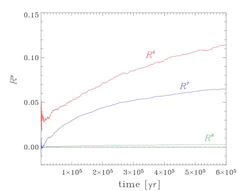
Figure 1: Time evolution of the residuals of the Strömgren sphere radius, ${\mathcal{R}}^{y}$, for a run with $N_{p}=10^{y}$ and $y$=6,7,8, calculated with respect to $N_{p}=10^{9}$ (see text for details).

In this Section, we present a set of tests to illustrate the performances of CRASH in a wide range of astrophysical and cosmological contexts. Radiative transfer problems in three dimensions do not have, in general, analytical solutions except for some simple cases; for this reason testing quantitatively a radiative transfer code is a challenging purpose. As a first test we consider the case of a monochromatic point source embedded in a pure-hydrogen homogeneous gas, with the ionized component at constant temperature. This idealized case of an isothermal Strömgren sphere, has the advantage of being directly comparable to an analytical solution of the problem (e.g. Spitzer 1978). Hence, it is possible to verify the accuracy of the code in reproducing the time evolution of the simulated system and its performances in a large range of gas densities. A second test is designed to check the reliability of the algorithm in calculating the temperature and ionization structure of a gas of primordial H/He composition.

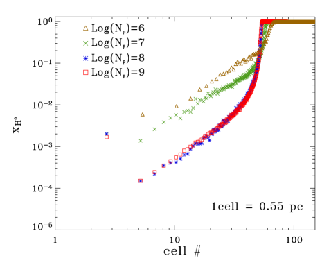
Figure 2: Neutral hydrogen fraction, $x_{{\rm H}^{0}}$, as a function of the distance from the source in cell units. The points represent a subsample of grid points for runs with: $N_{p}=10^{6},10^{7},10^{8},10^{9}$ (triangles, crosses, asterisks and squares).

As no analytical solution is available for this more realistic case, as a check, we compare our results with the ones of the 1-D RT code CLOUDY94, available on the web. The above test is extended to the case of two point sources with largely different luminosities. This problem turns out to be a difficult benchmark for RT codes (see Gnedin & Abel 2001 for a discussion). Finally, we study the case of a dense, very optically thick slab illuminated by a power-law background radiation: our main aim is to show how CRASH performs when confronted with the problem of the diffuse radiation field produced by recombining gas (shadowing).
To test even more complex problems (i.e. time evolution, inhomogeneous density field) it is instead necessary to compare results obtained with different RT codes; such an attempt (dubbed TSU³) is currently under development.

 

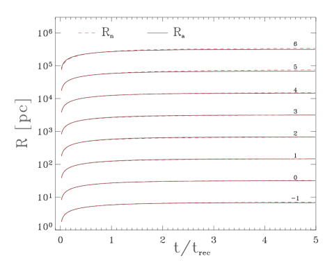
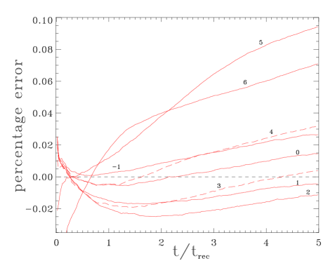
Figure 3: Left: time evolution of the numerical H_II region radius $R_{n}$ (dashed lines) compared with the analytical solution $R_{a}$ (solid). The curves refer to eight different values of $n_{H}=10^{-q}$ cm^-3 and are labeled with the index, $q$, of the corresponding density. Right: percentage errors on the numerical radius with respect to the analytical one for the same runs (and labels) as in the left panel.

3.1 Pure Hydrogen, Isothermal Strömgren Sphere

As mentioned, we first test the code against the analytical solution for the time evolution of the radius of the H_II region produced by a monochromatic source with constant ionizing rate and expanding in a homogeneous medium. The comparison requires an helium abundance equal to zero and a constant temperature in the H_II region; we fixed it equal to $T=10^{4}$ K. The (homogeneous) density field in the simulation box is initialized with a hydrogen number density of $n_{H}=1$ cm^-3; the cartesian grid, which has a linear size $L_{box}=70$ pc, is composed of $N_{c}^{3}=128^{3}$ cells. This density value has been chosen in order for the diffuse (recombination) radiation effects to be evident, so to test the corresponding implementation. The monochromatic source emits photons with energy equal to 13.6 eV, is located at the center of the box and has an ionizing photon rate $\dot{N}_{\gamma}=10^{48}$s^-1. The ionized hydrogen fraction is initialized at collisional equilibrium at $T=10^{4}$ K, i.e. $x_{{\rm H}^{+}}=1.2\times 10^{-3}$. To ensure that equilibrium configuration is achieved the simulation is carried out for a physical time $t_{s}=6\times 10^{5}$ yrs, roughly equal to five recombination times.

The H_II region equivalent radius, $R_{n}$, can be derived as $R_{n}=(3V_{n}/4\pi)^{1/3}$, where $V_{n}$ is the volume of the ionized region. The contribution of each cell $(x,y,x)$ to $V_{n}$ is assumed to be a fraction of the cell volume equal to its ionization fraction $x_{\rm H^{+}}(x,y,z)$:

$$V_{n}=\sum_{ix,iy,iz}x_{H^{+}}(\Delta x)^{3}.$$ (18)

As a single cell could be brought to ionization equilibrium in several time steps, this approach guarantees that the volume of the H_II region is not overestimated as the contribution of the partially ionized cells at the edge of the I-front is included.

To check for convergency, we run four simulations with increasing $N_{p}$. Fig. 1 shows the residual, ${\mathcal{R}}^{y}$, of a given run with respect to the highest resolution run ($N_{p}=10^{9}$), defined as:

$${\mathcal{R}}^{y}=\frac{R_{n}^{y}-R_{n}^{9}}{R_{n}^{9}},$$ (19)

where $y=6,7,8$ refers to the run with $N_{p}=10^{y}$. Good convergency is achieved already for $N_{p}=10^{7}$, when the residual is $\lower 2.15277pt\hbox{$\;\buildrel<\over{\sim}\;$}7$%.
In Fig. 2, the equilibrium neutral hydrogen fraction, $x_{{\rm H}^{0}}=n_{{\rm H}^{0}}/n_{\rm H}$, profile is shown for the four runs. In this case, a higher number of photon packets ($N_{p}\approx 10^{8}$) is needed to reach a good level of convergency. This result suggests that applications which require the determination of the volume ionization structure (as cosmic reionization) are less demanding than problems that require the correct value of neutral hydrogen fraction (i.e. Ly$\alpha$ forest simulations). Thus, depending on the application and the desired accuracy, the required number of photon packets might vary; anyway CRASH converges for a reasonable number of photon packets. As $N_{p}=10^{7}$ already gives good convergency of the calculated numerical radius to be compared with the analytical solution, in the following applications we will adopt this value, unless otherwise stated.

The time evolution of $R_{n}$ can now be compared with the classical analytical solution (Spitzer, 1978):

$$R_{a}(t)=R_{S}(1-e^{-n_{H}\alpha_{B}t})^{1/3},$$ (20)

where $R_{S}=\left(3\dot{N}_{\gamma}/4\pi n_{H}^{2}\alpha_{B}\right)^{1/3}$ is the Strömgren radius and $\alpha_{B}$ is the hydrogen recombination coefficient to levels higher than the first. The comparison of our numerical results for $R_{n}$ against the analytical solution, has been performed for eight different values of the density in the range $n=10^{-6}-10$ cm^-3. In each run $N_{p}$, $N_{c}$ and $\dot{N}_{\gamma}$ are kept constant, as specified above. The source has been located at a corner of the simulation box (of linear size equal to $6R_{S}/5$), to maximize spatial resolution. With the physical simulation time set to $t_{s}=5t^{B}_{rec}$, the equilibrium configuration is reached within $0.25$% of the total computational time, according to eq. (20). As $N_{cr}$ is fixed for all the runs, the accuracy itself is the same, as far as the photon packet distribution and the discretization errors are concerned. Similarly, the ratio $N_{\gamma}/N_{a}$, which determines the accuracy to which the continuity of the photoionization process is reproduced, is the same for all the runs. In fact,

$$N_{\gamma}/N_{a} = (\dot{N}_{\gamma}t_{s}N_{p}^{-1})/(n_{H}{\Delta x}^{3})$$

$$\propto n_{H}^{-1}/\left[n_{H}(n_{H}^{-2/3})^{3}\right]={\rm const},$$

Finally, the ratio between the ionizing photon emission rate and the rate of physical processes reproduced as continuous (recombinations, collisional ionizations etc.) in a given cell increases with density: $\dot{N}_{\gamma}(L_{box})^{-2}t_{min}\propto\dot{N}_{\gamma}(n_{H}^{-2/3})^{-2}n_{H}^{-1}\propto n_{H}^{1/3}$. Hence, if $\dot{N}_{\gamma}$ remains constant, the accuracy of the results decreases towards lower densities for the reasons explained in Section 2.5.

This conclusion is supported by the numerical experiments shown in Fig. 3, showing the evolution of the numerical radius, $R_{n}$ (dotted line), compared with the analytical solution, $R_{a}$ (solid line), for eight values of the density considered. The agreement is remarkably good. For densities $>10^{-4}$cm^-3 errors remain through the entire simulation $\lower 2.15277pt\hbox{$\;\buildrel<\over{\sim}\;$}3$%; for lower densities they increase, according to expectations following the previous discussion, up to $\approx 10$% for $n_{H}=10^{-5}-10^{-6}$ cm^-3. We point out that these runs have the minimum resolution required to achieve convergency and that accuracy can be easily improved using a larger value for $N_{p}$.

These tests, embracing 8 dex in density, demonstrate that CRASH is quite robust and accurate over a wide range of physical conditions.

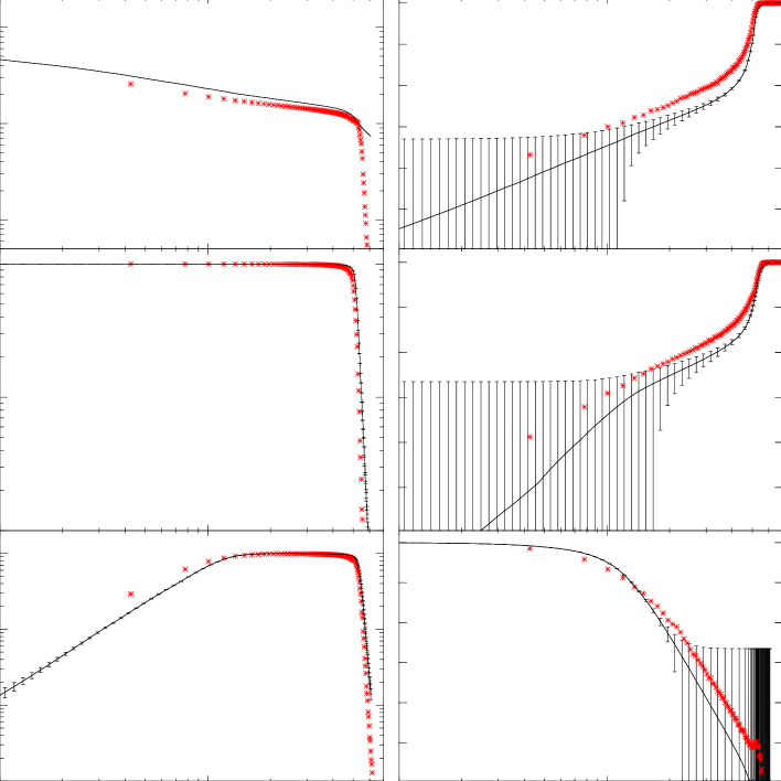
Figure 4: Comparison between the equilibrium configurations obtained by CRASH (points) and CLOUDY94 (solid lines) for different physical quantities, as a function of distance from the point source in cell units. The errors refer to the CLOUDY94 results and are evaluated as explained in the text.

3.2 Realistic Strömgren Spheres

Next, we test the CRASH scheme for the calculation of temperature and helium ionization. As no analytical solution is available, we compare the results with those obtained with the public code CLOUDY94, a 1-D radiative transfer code which calculates equilibrium configurations of the various species. The physics included in the two codes is slightly different. CLOUDY94 treats atoms and ions as multilevel systems, while we consider all species as one-level systems; furthermore CLOUDY94 includes some physical processes, like heat conduction and gas pressure effects, which are not included in CRASH . We consider a point source, emitting as a black body at $T=60000$ K with a luminosity $L=10^{38}$ erg s^-1, located at the center of the simulation box and embedded in a homogeneous density field with $n=1$ cm^-3 composed of hydrogen (90 % by number) and helium (10 %). The gas is initially completely neutral and at a temperature $T=10^{2}$ K in the entire simulation box, whose linear dimension has been fixed to $L_{box}=128$ pc. As an accurate determination of the neutral fractions and temperature inside the ionized regions requires $N_{p}\geq 10^{8}$ (see previous Section), we adopt $N_{p}=10^{8}$. Moreover, spherical symmetry is required to degenerate our 3-D solution to the 1-D geometry adopted by CLOUDY94. The comparison is performed at a time $t_{s}=6\times 10^{5}$ yr $\approx 5t_{rec}^{B}$ (where $t_{rec}^{B}$ is the characteristic time scale for hydrogen recombination to levels other than the first), when the equilibrium configuration has been reached. In Fig. 4 the comparison between the results of the CLOUDY94 (solid lines) and CRASH (points) is shown. The value of the different physical quantities is plotted as a function of the distance from the source, expressed in cell units, $\Delta x=1$ pc. The points represent spherically averaged CRASH outputs. Despite the differences between the two codes, a remarkably good agreement is obtained. In particular, the temperature profiles agrees within 10% of the CLOUDY solution, except from the warm tail extending beyond the location of the ionization front produced by CLOUDY94. The nature of this feature is unclear, but it can be probably imputed to heat conduction, implemented in CLOUDY94, which cause an heat transfer across the ionization front where the temperature gradient is very high.

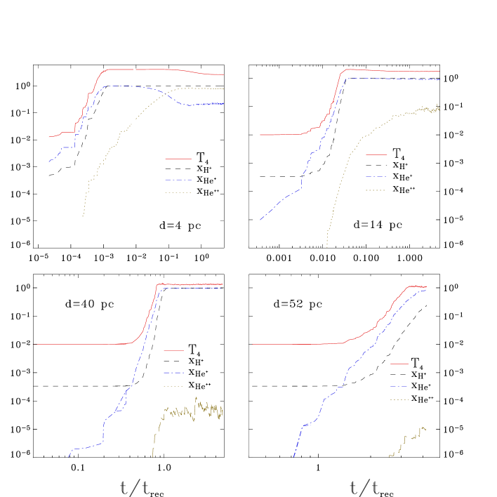
Figure 5: Evolution of the temperature, $T$ (in units of $10^{4}$ K; solid lines) and ionization fractions for $x_{H^{+}}$ (dashed), $x_{He^{+}}$ (dotted-dashed) and $x_{He^{++}}$ (long dashed), in four fixed cells at different distances from the source, $d$=1, 14, 40 and 52 pc.

As for the ionization fractions, the errors plotted on the CLOUDY94 curves are evaluated as follows. At some distances from the source, the CLOUDY94 calculation gives the unphysical results $(x_{H^{+}}+x_{H^{0}})>1$ or $(x_{He^{0}}+x_{He^{+}}+x_{He^{++}})>1$; we then assume the errors to be the maximum value of the quantities $\left[(x_{H^{+}}+x_{H^{0}})-1\right]$, for hydrogen species, and $\left[(x_{He^{0}}+x_{He^{+}}+x_{He^{++}})-1\right]$ for helium species. The errors on the CRASH results are shown by the scatter of the plotted points, which is more significant for the neutral fractions as a result of the discretization error connected to continuous process. The $x_{H^{0}}$ and $x_{He^{0}}$ profiles produced by the two codes are characterized by the same trend. The CRASH results tend to overpredict these quantities with respect to CLOUDY94 on average by 20-30%; this is also the case for the $x_{He^{+}}$, and is likely due to differences in the expressions for the rate coefficients adopted. For example, at $T=10^{4}$ K the CRASH total hydrogen recombination rate (see Appendix B) is equal to 5.097$\times 10^{-13}$ cm³ s^-1, while that adopted by CLOUDY (see Table 20 of CLOUDY90 manual) is 4.17$\times 10^{-13}$ cm³ s^-1, i.e. a 20% discrepancy. Our higher value is consistent with the larger abundance of H⁰ found inside the H_II. The $x_{H^{+}}$ profiles are in perfect agreement, as well as the $x_{He^{++}}$ profiles which appear to be in very good agreement within the errors.

To get more insights on the numerical technique adopted, we plot in Fig. 5 the evolution of the temperature and ionization fractions for the various species in four fixed cells at different distances from the source ($d=4,14,40$ and 52 pc). It is important to note that the continuity of the photoionization (photoheating) process is well reproduced at all distances; also, cells at different distances start to be ionized at different times, as the I-front propagates into the density field. Only in the cell closest to the source the radiation field at energies higher than 4 Ryd is strong enough to significantly doubly ionize He; at 14 pc from the source He⁺ is only partially ionized, and in the two most distant cells He⁺⁺ aboundance is almost negligible.

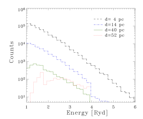
Figure 6: Frequency distribution of the photon packets, weighted by their photon content, seen by the same four cells of Fig. 5 over the entire simulation.

The flux depletion and the progressive filtering of the spectrum by the intervening medium, are further illustrated by Fig. 6, where we plot the frequency distribution of photon packets crossing the same four cells as above during the entire simulation, weighted by their photon content. Moving to regions farther from the source, the ionizing flux decreases, as expected, due to the combined effect of geometrical dilution and photoelectric absorption; this last process also causes the filtering effect resulting in the progressive hardening of the spectrum. Again, we note that packets with energy above 4 Ryd are heavily depleted in distant regions.

These tests allow us to conclude that CRASH reliably computes, on limited computational times (the discussed simulation took a few hours on a 1 GHz workstation), the physical quantities of a photoionized gas of primordial composition and, when confronted to state-of-the-art 1-D equilibrium codes as CLOUDY94, produces results of comparable accuracy level.

As a final remark, we note that the presented tests constitute a particularly difficult physical benchmark due to the relatively high densities and soft source spectrum.

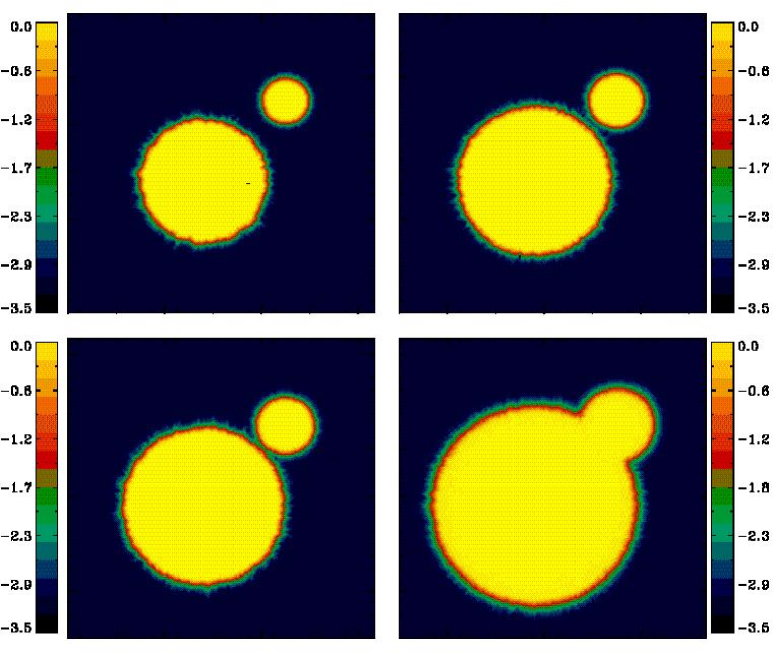
Figure 7: Slice of the simulation box through the planes containing the source locations showing the ionized hydrogen fraction, $x_{\rm H^{+}}$, distribution at four different simulation times: $(0.3,0.6,0.9,3)\times t_{rec}^{B}$ (from left to right and top to bottom).

3.3 Multiple Point Sources

As a third test we run the case of multiple radiation sources in the box. Again, we consider a homogeneous H/He density field with $n=1$ cm^-3, $N_{c}=128$, $N_{p}=10^{8}$ and $L_{box}=160$ pc. Two sources are embedded in the computational volume: one with $L_{1}=10^{38}$ erg s^-1, and a weaker one with $L_{2}=L_{1}/27$, both with a $T=60000$ K black-body spectrum. The temperature and ionization fractions fields are initialized as in the previous test. We follow the evolution of this system for a time $t_{s}=4.5\times 10^{5}$ yr $\approx 3.4t_{rec}^{B}$.

In Fig. 7 we show the ionized hydrogen fraction distribution in a slice of the simulation box through the plane containing the source locations. The panels refer to four different simulation times: $(0.3,0.6,0.9,3)\times t_{rec}^{B}$. The H_II regions around each source evolve independently until they merge at $t\simeq t_{rec}^{B}$. Once the H_II regions overlap, photons from one source can change the properties of the ionized region previously produced by the other one. In particular, we notice that the I-front curvature of the smaller H_II region is changed in the overlapping region.

 

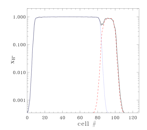
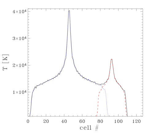
Figure 8: Left: Ionized hydrogen fraction along a direction parallel ($\approx 10$ cells away) to the one connecting the two sources and passing trough the I-fronts intersection region. The three lines refer to simulations in which either the stronger (dashed line) or the weaker source (dotted-dashed) were turned off; the third cut (solid) is through the simulations in which both sources are active. Right: Temperature along the line connecting the two sources; the notation for the curves is the same as in the left panel.

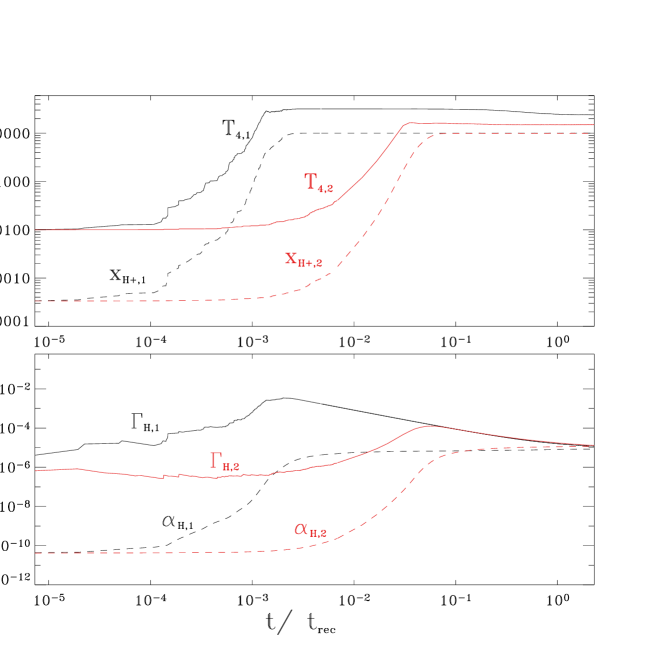
Figure 9: Upper panel: Time evolution of the temperature (solid), hydrogen ionization fraction (dashed) for two cells located at a distance $d=5$ pc from each source. The label 1 (2) on the curves refer to the cell at 5 pc from the the source wiht luminosity $L_{1}$ ($L_{2}$=$L_{1}/27$). Lower panel: As above, but for the photoionization (solid) and recombination (dashed) rates.

This effect is better illustrated by Fig. 8 (left panel), where a 1-D cut of the ionized hydrogen fraction along a direction parallel ($\approx 10$ cells away) to that connecting two sources is shown. The three lines refer to simulations in which either one or the other source were turned off and in which both sources are active. As described above, in the cumulative curve an enhancement of the H⁺ fraction is clearly visible both in the overlapping region and on the far side of the smaller H_II region due to percolating photons coming from the stronger source. A similar effect is visible in the temperature profiles along the line of sight connecting the two sources, plotted in the right panel of Fig. 8. In the overlapping region the temperature is larger than for the case of a single source.

In order to understand the reason for the difference in the temperature profiles within the H_II regions of the two sources we have performed an additional check. The heating rate associated with photoionizations of the species $A$ can be written as ${\cal H}_{A}=\Gamma_{A}\langle h\nu\rangle$, where $\langle h\nu\rangle$ is the mean energy of the photoelectrons. As the spectrum is the same, ${\cal H}_{A}$ only depends on the photoionization rate. The temperature results from the balance of such photoheating with radiative losses. In turn, we have checked that the latter are largely dominated by the recombination cooling rate, which can also be written as the product of the recombination rate and the mean energy lost per recombining electron. Fig. 9 shows the time evolution of the temperature, hydrogen ionization fraction (upper panel), photoionization and recombination rates (lower panel) for two cells located at a distance $d=5$ pc from each source. The different luminosity of the sources results in a different gas thermal/ionization history, the cell illuminated by the most luminous source reaching equilibrium earlier. The photoionization rate increases smoothly with time, due to the decrease of the intervening opacity, until it reaches a maximum; thereafter it decreases because of the lack of absorbers. The temperature equilibrium value is reached in both cases slightly before the recombination rate reaches a plateau at $\approx 10^{-5}$ yr^-1; this value is the same for the two sources as it essentially depends only on the gas density (the tiny deviation seen at large evolutionary times is due to the temperature dependence of the recombination coefficient). However, the photoionization rate at that stage is larger (by roughly a factor $L_{1}/L_{2}$=27) for the more luminous source than for the fainter one. This extra net heating explains the temperature difference. It is also worth noting that asymptotically the photoionization and the recombination rates become equal as expected from the equilibrium condition for a Strömgren sphere.

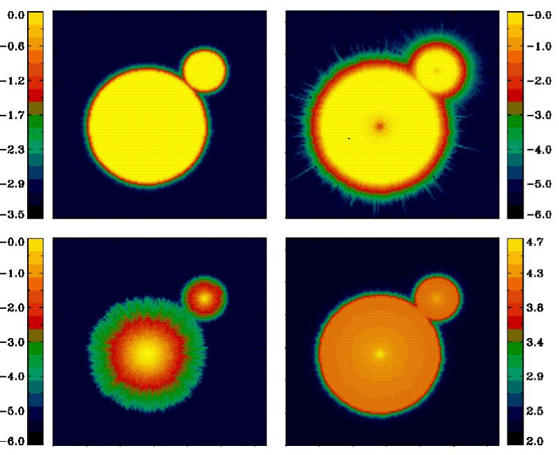
Figure 10: Slices of the simulation box through the plane containing the sources locations showing $x_{H^{+}}$, $x_{He^{+}}$, $x_{He{{}^{++}}}$ and temperature distributions (from left to right and from top to bottom) at the end of the simulation, $t=3.4t_{rec}^{B}$.

Finally, in Fig. 10 we plot 2-D maps of the $x_{H^{+}}$, $x_{He^{+}}$, $x_{He^{++}}$ and temperature distributions at the end of the simulation. Due to the larger mean free path typical of He⁰ ionizing photons, the He⁺ I-front is wider than the H⁺ one, and it is also smoother due the flatter spectrum at $h\nu\geq 24.6$ eV. Moreover, the He⁺ I-front appears to be more affected by numerical noise because of the poorer sampling of the helium ionizing region of the spectrum. This is even more evident in the He⁺⁺ distribution for which the I-front is jagged in the outer parts, where ionization balance is governed by the very high energy tail of the power spectrum. Nevertheless the calculation correctly reproduces the higher He⁺ ionization level around to the stronger source.

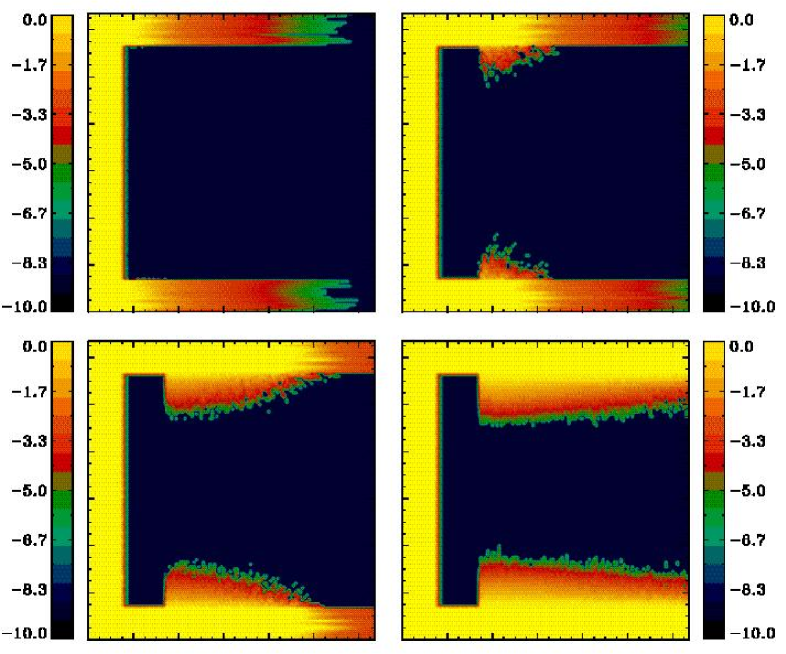
Figure 11: Maps of the $x_{H^{+}}$ distribution at four different simulation times: $(0.2,0.4,0.9,2)\times t_{rec}^{B}$ (from top to bottom and from left to right). The test refers to a region with an overdensity of $10^{3}$ and a dimension of 128$\times$100$\times$20 cells embedded in a homogeneous medium and exposed to a plane parallel ionization front traveling from left to right (see text for details).

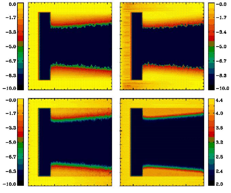
Figure 12: Maps of $x_{H^{+}}$, $x_{He^{+}}$, $x_{He{{}^{++}}}$ and temperature distributions (from left to right and from top to bottom) at the end of the simulation.

3.4 Shadowing of background radiation

As a final test, we study the case of a gas ionized by a power-law background radiation field. Our main aim is to demonstrate the ability of CRASH to deal with the problem of diffuse recombination radiation. The density field has been initialized with a high density region ($n$=1 cm^-3) of dimension 128$\times$100$\times$20 cells, embedded in an homogeneous gas with $n=10^{-3}$ cm ^-3. The density field is exposed to a plane parallel ionization front traveling orthogonally to the overdense slice. The background spectrum has a power-law shape, $J_{\nu}=J_{0}(\nu/\nu_{th,H^{0}})^{-\alpha}$, with $J_{0}=10^{-22}$ erg cm^-2 s^-1 Hz^-1 and $\alpha=-1.4$. The gas composition is the same as in the previous tests. The gas is initially completely neutral and at a temperature $T=10^{2}$ K in the entire simulation box; the physical simulation time is $t_{s}=3\times 10^{8}$ yr$\approx 4.3t_{rec}^{B}$, the box linear size is $L_{box}=6.6$ kpc; moreover, $N_{p}=5\times 10^{7}$ and $N_{c}=128$.
Fig. 10 shows maps of the ionized hydrogen fraction distribution, orthogonal to the overdense slice, at four different simulation times: $(0.2,0.4,0.9,2)\times t_{rec}^{B}$. The I-front initially propagates into the low density field, but it is stopped at the edge of the slice by the high recombination rate, producing a shadow behind it. The I-front is very smooth due the power-law spectrum of the ionizing background. As the simulation proceeds, the diffuse radiation produced by recombinations in the ionized gas, begin to ionize the low density region behind the high density slice. The diffuse radiation then propagates into the shadowed region, ionizing gas that would otherwise remain neutral. Finally, Fig. 11 shows maps for the final $x_{H^{+}}$, $x_{He^{+}}$, $x_{He^{++}}$ and temperature distributions. The hard spectrum is able to ionize almost completely helium to He⁺⁺ in the regions exposed to direct radiation, whereas the diffuse radiation is not hard enough to produce the same effect. In the He⁺⁺ distribution (lower-left panel), a clear separation between the gas ionized by either direct or diffuse radiation is visible. A similar signature is present also in the temperature map, again caused by the fact that diffuse photons have typical energies confined in a narrow band above ionization thresholds of the three absorbers; as a consequence, little energy is available to photoheat the gas. In conclusion, although necessarily qualitative due to the lack of precise solutions to this problem, the shadowing experiment performed here seems to yield physically plausible results.

4 Summary

We have presented an updated version of CRASH , a 3-D RT code evaluating the effects of an ionizing radiation field propagating through a given inhomogeneous H/He density field on the physical conditions of the gas. The code, based on a Monte Carlo technique, self-consistently calculates the time evolution of gas temperature and ionization fractions due to an arbitrary number of point/extended sources and/or diffuse background radiation with given spectra. In addition, the effects of diffuse ionizing radiation following recombinations of ionized atoms have been included. The code has been primarily developed to study a number of cosmological problems, such as hydrogen and helium reionization, physical state of the Ly$\alpha$ forest, escape fraction of Lyman continuum photons from galaxies, diffuse Ly$\alpha$ emission from recombining gas, etc. However, its flexibility allows applications that could be relevant to a wide range of astrophysical problems. The code architecture is sufficiently simple that additional physics can be easily added using the same algorithms already described in this paper. For example, dust absorption/re-emission can be included with minimum effort; molecular opacity and line emission, although more complicated, do not represent a particular challenge given the numerical scheme adopted. Obviously, were such processes added, the computational time could become so long that parallelization would be necessary. This would be required also when CRASH will be coupled to a hydrodynamical code to study the feedback of photo-processes onto the (thermo-)dynamics of the system. This perspective development looks quite encouraging: in fact, Monte Carlo schemes are by construction extremely suitable for parallel computations, as the packet load can be distributed in a straightforward manner to processors, limiting the inter-communication problems among them to a very minimum. Clearly, this is a noticeable advantage of the adopted scheme over those based on full solution of the RT equations. This study is already under work and its implementation will be presented in a forthcoming communication.

To demonstrate the performances, accuracy and robustness of the code we have studied in detail four different test cases designed to ascertain specific aspects of RT: (i) pure hydrogen isothermal Strömgren spheres; (ii) realistic Strömgren spheres; (iii) multiple overlapping point sources, and (iv) shadowing of background radiation. When possible, a detailed quantitative comparison of the results against either analytical solutions or 1-D standard photoionization codes has been made showing a remarkable level of agreement ($\;\buildrel<\over{\sim}\;$ few percent). For more challenging tests the code yields physically plausible results, which could be checked only by comparison with other similar codes.

This work was partially supported by the Research and Training Network ‘The Physics of the Intergalactic Medium’ set up by the European Community under the contract HPRN-CT2000-00126 RG29185.

Appendix A Monte Carlo sampling

The Monte Carlo (MC) method, extensively used in many field of scientific research, allows to sample with great efficiency physical quantities with a given Probability Distribution Function (PDF). Here we outline the basic principles on which the MC sampling technique is based. Let us consider a variable $q$ having values in the interval $[a,b]$, representing a physical quantity distributed according to a PDF, $f(q)$, normalized to $\int_{a}^{b}f(q)dq=1$. The PDF is defined so that the probability of having a value $q$ in the range $[q^{\prime},q^{\prime}+dq]$ is $f(q^{\prime})dq$. Let us also introduce the cumulative probability $P(q^{\prime})$, defined as:

$$P(q^{\prime})=\int_{a}^{q^{\prime}}f(q)dq,$$ (22)

which measures the probability that the previous value of $q$ will yield a value lower or equal to $q^{\prime}$. Given the above normalization, $P(q^{\prime})\leq 1$ for each $q^{\prime}$ in $[a,b]$.

Once the PDF is given, a number ${\cal R}$ is randomly extracted in the interval $[0,1]$. Then, $q^{\prime}$ is derived setting ${\cal R}=P(q^{\prime})$ and inverting the integral in eq. 22. In this way the probability of obtaining the value $q^{\prime}$ when extracting randomly a number in [0,1], corresponds exactly to $f(q^{\prime})$.

If the number of extractions is large enough, it is possible to obtain a statistical population of values which reproduces with great accuracy the given PDF. The main advantage of this technique lies in the ability to sample arbitrary distribution functions by simply randomly sampling the interval $[0,1]$, an easy and cheap algorithm to implement.

Appendix B Rate Coefficients and Cross Sections

In this Section we list the rate coefficients and the cross sections adopted by CRASH , for all the physical processes included.

• Photoionization cross sections    [cm^-2]     (1)
  

  $${\rm H}^{0}\;:\;\sigma_{H^{0}}(\nu)=6.3\times 10^{-18}(\nu/\nu_{th,{\rm H}^{0}})^{-3}\;\;\;\;\;\;\;\;\;\;\;\;\;\;\;\;\;\;\;\;\;\;\;\;\;\;\;\;\;\;\;\;\;\;\;\;\;\;\;\;\;\;\;\;\;\;\;\;\;\;\;\;\;\;\;\;\;\;\;\;\;\;\;\;\;$$

  $${\rm He}^{0}:\sigma_{He^{0}}(\nu)=7.2\times 10^{-18}[1.66(\nu/\nu_{th,{\rm He}^{0}})^{-2.05}\;\;\;\;\;\;\;\;\;\;\;\;\;\;\;\;\;\;\;\;\;\;\;\;\;\;\;\;\;\;\;\;\;$$

  $$\;\;\;\;\;\;\;\;\;\;\;\;\;\;\;\;\;+0.66(\nu/\nu_{th,{\rm He}^{0}})^{-3.05}]\;\;\;\;\;\;\;\;\;\;\;\;\;\;\;\;\;\;\;\;\;$$

  $${\rm He}^{+}:\sigma_{He^{+}}(\nu)=1.58\;\times\;10^{-18}(\nu/\nu_{th,{\rm He}^{+}})^{-3}\;\;\;\;\;\;\;\;\;\;\;\;\;\;\;\;\;\;\;\;\;\;\;$$

  
  

• Recombination rates    [cm³ s^-1]     (2)
  

  $${\rm H}^{0}\;:\;\alpha_{H^{0}}(T)=8.40\times 10^{-11}T^{-1/2}\left(\frac{T}{10^{3}}\right)^{-0.2}\left[1+\left(\frac{T}{10^{6}}\right)^{0.7}\right]^{-1}$$

  $${\rm He}^{0}:\alpha_{He^{0}}(T)=1.50\times 10^{-10}T^{-0.6353}\;\;\;\;\;\;\;\;\;\;\;\;\;\;\;\;\;\;\;\;\;\;\;\;\;\;\;\;\;\;\;\;\;\;\;\;\;\;\;\;\;\;\;\;\;\;\;\;\;\;\;\;\;\;\;\;$$

  $${\rm He}^{+}:\alpha_{He^{+}}(T)=3.36\times 10^{-10}T^{-1/2}\left(\frac{T}{10^{3}}\right)^{-0.2}\left[1+\left(\frac{T}{10^{6}}\right)^{0.7}\right]^{-1}$$

  
  

• Collisional ionization rates    [cm³ s^-1]     (2)
  

  $${\rm H}^{0}\;:\;\gamma_{H^{0}}(T)=5.85\times 10^{-11}T^{1/2}\left[1+\left(\frac{T}{10^{5}}\right)^{1/2}\right]^{-1}e^{-157809.1/T}$$

  $${\rm He}^{0}:\gamma_{He^{0}}(T)=2.38\times 10^{-11}T^{1/2}\left[1+\left(\frac{T}{10^{5}}\right)^{1/2}\right]^{-1}e^{-285335.4/T}\$$

  $${\rm He}^{+}:\gamma_{He^{+}}(T)=5.68\times 10^{-12}T^{1/2}\left[1+\left(\frac{T}{10^{5}}\right)^{1/2}\right]^{-1}e^{-631515/T}$$

  The cooling function, $\Lambda(T,n_{e},n_{H^{0}},n_{H^{+}},n_{He^{0}},n_{He^{+}},n_{He^{++}})$, is calculated including the contribution of the following radiative processes:
  

• Collisional ionization cooling    [erg cm³ s^-1]     (2)
  

  $${\rm H}^{0}\;:\;\zeta_{H^{0}}(T)=1.27\times 10^{-21}T^{1/2}\left[1+\left(\frac{T}{10^{5}}\right)^{1/2}\right]^{-1}e^{-157809.1/T}$$

  $${\rm He}^{0}:\zeta_{He^{0}}(T)=9.38\times 10^{-22}T^{1/2}\left[1+\left(\frac{T}{10^{5}}\right)^{1/2}\right]^{-1}e^{-285335.4/T}$$

  $${\rm He}^{+}:\zeta_{He^{+}}(T)=4.95\times 10^{-22}T^{1/2}\left[1+\left(\frac{T}{10^{5}}\right)^{1/2}\right]^{-1}e^{-631515/T}$$

  
  

• Recombination cooling    [erg cm³ s^-1]     (2)
  

  $${\rm H}^{0}\;:\;\eta_{H^{0}}(T)=8.70\times 10^{-27}T^{1/2}\left(\frac{T}{10^{3}}\right)^{-0.2}\left[1+\left(\frac{T}{10^{6}}\right)^{0.7}\right]^{-1}$$

  $${\rm He}^{0}:\eta_{He^{0}}(T)=1.55\times 10^{-26}T^{0.3647}\;\;\;\;\;\;\;\;\;\;\;\;\;\;\;\;\;\;\;\;\;\;\;\;\;\;\;\;\;\;\;\;\;\;\;\;\;\;\;\;\;\;\;\;\;\;\;\;\;\;\;\;\;\;\;\;\;\;\;$$

  $${\rm He}^{+}:\eta_{He^{+}}(T)=3.48\times 10^{-26}T^{1/2}\left(\frac{T}{10^{3}}\right)^{-0.2}\left[1+\left(\frac{T}{10^{6}}\right)^{0.7}\right]^{-1}$$

  
  

• Collisional excitation cooling     (2)
  

  $${\rm H}^{0}\;:\;\psi_{H^{0}}(T)=7.5\times 10^{-19}\left[1+\left(\frac{T}{10^{5}}\right)^{1/2}\right]^{-1}e^{-118348/T}\;\;\;\;$$

  $\;\;\;\;\;\;\;\;[\psi_{H^{0}}]$=[erg cm³ s^-1]

  $${\rm He}^{+}:\psi_{He^{+}}(T)=5.54\times 10^{-17}T^{-0.397}\left[1+\left(\frac{T}{10^{5}}\right)^{1/2}\right]^{-1}e^{-473638/T}$$

  $\;\;\;\;\;\;\;\;[\psi_{He^{+}}]$=[erg cm³ s^-1]

  $${\rm He}^{0}:\psi_{He}(T)=9.10\times 10^{-27}T^{-0.1687}\left[1+\left(\frac{T}{10^{5}}\right)^{1/2}\right]^{-1}e^{-13179/T}$$

  $\;\;\;\;\;\;\;\;[\psi_{He}]$=[erg cm⁶ s^-1]
  

  The above expressions are for excitations to all H⁰ levels, to $n=2$ for He⁺ and to the $n=2,3,4$ He⁰ triplets (of the He⁰($2^{3}$S) state, supposed to be populated by He⁺ recombinations)
  

• Bremsstrahlung cooling    [erg cm^-3 s^-1]     (3)
  

  $$\beta(T)=1.42\times 10^{-27}T^{1/2}\left[n_{H^{+}}+n_{He^{+}}+4n_{He^{++}}\right]n_{e}$$

  
  

• Compton cooling/heating    [erg cm^-3 s^-1]     (4)
  

  $$\varpi(T)=1.017\times 10^{-37}T_{\gamma}^{4}\left[T-T_{\gamma}\right]n_{e}\;\;\;\;\;\;\;\;\;\;\;\;\;\;\;\;\;\;\;\;\;\;\;\;\;$$

  
  

  References: (1) Osterbrok 1989; (2) Cen 1992; (3) Black 1981; (4) Haiman et al. 1996

References

- [1] Abel, T., Norman, M. L. & Madau, P. 1999, ApJ, 523, 66
- [2] Abel, T. & Wandelt, B. D. 2002, MNRAS, 330, L53
- [3] Benson, A.J., Nusser, A., Sugiyama, N. & Lacey, C.G. 2001, MNRAS, 320, 153
- [4] Bianchi S., Ferrara A. & Giovanardi C., 1996, ApJ, 523,
- [5] Bianchi S., Ferrara A., Davis J. & Alton P.,2000, MNRAS, 311, 601
- [6] Black, J.H., 1981, MNRAS, 197, 553
- [7] Cashwell, E. D., Evrett, C. J.,1959,A Practical Manual on the Monte Carlo Method for Random Walk Problems, Pergamon, New York
- [8] Cen, R. 1992, ApJS, 78, 341
- [9] Cen, R. 2002, ApJS, 141, 211
- [10] Chiu, W. A. & Ostriker, J. P. 2000, ApJ, 534, 507
- [11] Ciardi, B., Ferrara, A., Governato, F. & Jenkins, A. 2000, MNRAS, 314, 611 (CFGJ)
- [12] Ciardi, B., Ferrara, A., Marri, S. & Raimondo, G. 2001, MNRAS, 324, 381 (CFMR)
- [13] Ciardi, B., Stoehr, F. & White, S.D.M. 2003, astro-ph/0301293 (CSW)
- [14] Fan, X. et al. 2001, AJ, 122, 2833
- [15] Fan, X. et al. 2003, astro-ph/0301135
- [16] Ferrara, A., Bianchi, S., Dettmar, R. J. & Giovanardi, C., 1996, ApJ, 467, L69
- [17] Ferrara, A., Bianchi, S., Cimatti, A. & Giovanardi, C., 1999, ApJS, 123, 437
- [18] Gnedin, N. Y. 2000, ApJ, 535, 530
- [19] Gnedin, N. Y. & Abel, T. 2001, NewA, 6, 437
- [20] Gnedin, N. Y. & Ostriker, J. P. 1997, ApJ, 486, 581
- [21] Haiman, Z., Thoul, A. A., Loeb, A. 1996, ApJ, 464, 523
- [22] Haiman, Z. & Loeb, A. 1997, ApJ, 483, 21
- [23] Hu, E.M. et al. 2002, ApJ, 576, 99
- [24] Mihalas, D., 1978, Stella Atmospheres, W. H. Freeman and Company, San Francisco
- [25] Miralda-Escudé, J., Haehnelt, M. & Rees, M. R. 2000, ApJ, 530, 1
- [26] Osterbrok, D. E., 1989, Astrophysics of Gaseous Nebulae and Active Galactic Nuclei, Mill Valley: University science Books
- [27] Razoumov, A. O., Norman, M. L., Abel, T. & Scott, D. 2002, ApJ, 572, 695
- [28] Razoumov, A. & Scott, D. 1999, MNRAS, 309, 287
- [29] Sokasian, A., Abel, T. & Hernquist, L. E. 2001, NewA, 6, 359
- [30] Spitzer, L. Jr., 1978, Phisycal Processes in the Interstellar Medium, Jonh Wiley & Sons, New York
- [31] Umemura, M., Nakamoto, T. & Susa, H. 1999, in Numerical Astrophysics, eds.Miyama et al. (Kluwer: Dordrecht), p.43
- [32] Valageas, P. & Silk, J. 1999, A&A, 347, 1