Probing dark energy perturbations:
the dark energy equation of state and speed of sound as measured by WMAP

Abstract

We review the implications of having a non-trivial matter component in the universe and the potential for detecting such a component through the matter power spectrum and ISW effect. We adopt a phenomenological approach and consider the mysterious dark energy to be a cosmic fluid. It is thus fully characterized, up to linear order, by its equation of state and its speed of sound. Whereas the equation of state has been widely studied in the literature, less interest has been devoted to the speed of sound. Its observational consequences come predominantly from very large scale modes of dark matter perturbations ($k<0.01h\mathrm{Mpc}^{-1}$). Since these modes have hardly been probed so far by large scale galaxy surveys, we investigate whether joint constraints that can be placed on those two quantities using the recent CMB fluctuations measurements by WMAP as well as the recently measured CMB large scale structure cross-correlation. We find only a tentative 1$sigma$ detection of the speed of sound, from CMB alone, $c_{s}^{2}<0.04$ at this low significance level. Furthermore, the current uncertainties in bias in the matter power spectrum preclude any constraints being placed using the cross correlation of CMB with the NVSS radio survey. We believe however that improvements in bias through improved survey scales and depths in the near future will improve hopes of detecting the speed of sound.

I Introduction

With the recent unveiling of the Wilkinson Microwave Anisotropy Probe (WMAP) results, measuring the Cosmic Microwave Background (CMB) anisotropy Bennett03 , the on-going supernovae searches super and the upcoming completion of the Sloan Digital Sky Survey, amongst others, we are seeing a wealth of precision observational data being made available. To a great extent the standard $\Lambda$-CDM scenario fits the data well Spergel03 .

However, the WMAP data might suggest that some modifications to the standard scenario are needed. One possible hint at required modifications is the deficit of large scale power in the temperature map, and in particular, the low CMB quadrupole whose posterior probability is less than a few hundredth (see e.g. for possible interpretations Efstathiou03 ; Contaldi03 and Efstathiou03b for a discussion of this number). One possibility is that this lack of large scale power might point to some particular properties of the dark energy. The dominant contribution to fluctuations on these scales is the Integrated Sachs Wolfe (ISW) effect which describes the fluctuations induced by the passage of CMB photons through the time evolving gravitational potential associated to nearby ($z<5$) large scale structures (LSS). One property we expect of dark energy is that it suppresses the gravitational collapse of matter at relatively recent times, which in turn suppresses the gravitational potential felt by the photons, thereby leaving a signature in the ISW correlations. Since this signature is created by the time evolving potential associated with relatively close LSS, it should be intimately correlated with any tracer of LSS Kofman85 ; Crittenden96 . A positive detection of such a cross correlation using WMAP data, assuming a cosmological constant as the dark energy, has recently been measured Boughn03 ; Nolta03 ; Fosalba03 .

However the underlying cause of the dark energy is still unknown; and such observational inferences offer rich prospects for guiding and leading the theoretical effort. A wide variety of models have been proposed to explain observations, from the unperturbed cosmological constant, to a multitude of scalar field quintessence and exotic particle theories (see Peebles02 for a review).

Much effort has been put into determining the equation of state of dark energy, in an attempt to constrain and direct theories. Since the equation of state affects both the background expansion and the evolution of matter perturbations there are a wealth of complementary observations available (again see Peebles02 and references therein).

An equally insightful, but less investigated, characteristic of dark energy is the speed of sound within it. This does not affect the background evolution but is fundamental in determining a dark energy s clustering properties, through the Jeans scale. It will, therefore, have an effect on the evolution of fluctuations in the matter distribution.

Following the papers laying the foundations for cosmological perturbation theory Bardeen80 ; Kodama84 , the effect of the speed of sound on observables was considered in more detail: for the CMB and large scale structure Hu98 ; Hu99 and in the context of lensing Hu02 . Observational implications of the speed of sound in a variety of dark energy models have also recently been discussed: for example for k-essence Erikson01 ; Dedeo03 , condensation of dark matter Bassett02 and the Chaplygin gas, in terms of the matter power spectrum Sandvik02 ; Beca03 ; Reiss03 and combined full CMB and large scale structure measurements Bean03 ; Amendola03 .

Minimally coupled scalar field, quintessence models, commonly have a non-adiabatic speed of sound close or equal to unity (in units of c, the speed of light),(see for example Ferreira97 ). By contrast however, the adiabatic Chaplygin gas model,( e.g. motivated by a rolling tachyon Gibbons02 ) has a speed of sound directly proportional to the equation of state, both of which are approximately zero up until late times when the dark energy starts to dominate. It is conceivable therefore that distinctions between such models might be able to be made through the detection of a signature of the dark energy speed of sound: in the large scale ISW correlations, and in the cross correlation of the CMB with the distribution of large scale structure Crittenden96 .

In section II we briefly review parameters describing a general fluid and the issues that arise when establishing a fluid’s speed of sound. In section III we describe the implications of equation of state and speed of sound on perturbation evolution in the fluid and CDM. We consider a toy model with slowly varying equation of state and sound speed applicable in a wide variety of minimally coupled scalar field theories. In section IV we discuss the potential for detecting the speed of sound using late time perturbation evolution, in the ISW effect, through the autocorrelation of the CMB temperature power spectrum. In section V we extend the analysis to the cross correlation of the WMAP CMB data with distribution. Finally, in section VI we summarize our findings.

II The speed of sound within general matter

For a perfect fluid the speed of sound purely arises from adiabatic perturbations in the pressure, $p$, and energy density $\rho$ and the adiabatic speed of sound, $c_{a}^{2}$ is purely determined by the equation of state $w$,

$$w_{i} \equiv {p_{i}\over\rho_{i}}$$ (1)

$$c_{ai}^{2} \equiv {\dot{p}_{i}\over\dot{\rho}_{i}}=w_{i}-{\dot{w}_{i}\over 3{\cal H}(1+w_{i})}$$ (2)

where the subscript $i$ denotes a general specie of matter, where dots represent derivatives with respect to conformal time and where ${\cal H}$ is the Hubble constant with respect to conformal time.

In imperfect fluids, for example most scalar field or quintessence models, however, dissipative processes generate entropic perturbations in the fluid and this simple relation between background and the speed of sound breaks down and we have the more general relation

$$c_{si}^{2} \equiv {\delta p_{i}\over\delta\rho_{i}}.$$ (3)

In order to establish the speed of sound in these cases we must look to the full action for the fluid described often through the form of an effective potential. In this case, the speed of sound can be written in terms of the contribution of the adiabatic component and an additional entropy perturbation $\Gamma_{i}$ and the density fluctuation in the given frame $\delta_{i}$ Kodama84 ,

$$w_{i}\Gamma_{i} \equiv (c_{si}^{2}-c_{ai}^{2})\delta_{i}$$ (4)

$$= {\dot{p}_{i}\over\rho_{i}}\left({\delta p_{i}\over\dot{p}_{i}}-{\delta\rho_{i}\over\dot{\rho}_{i}}\right)$$ (5)

$\Gamma_{i}$ is the intrinsic entropy perturbation of the matter component, representing the displacement between hypersurfaces of uniform pressure and uniform energy density. In this paper, we are solely interested in probing the intrinsic entropy of the dark energy component. It is worth noting that in a multi-fluid scenario, in addition to the intrinsic entropy perturbations denoted by $\Gamma_{i}$, further contributions to the total entropy perturbation of the system can arise from the relative evolution of two or more fluids with different adiabatic sound speeds, and through non-minimal coupling (see for example Balakin03 ).

Whereas the adiabatic speed of sound, $c_{ai}$, and $\Gamma_{i}$ are scale independent, gauge invariant quantities, $c_{si}$ can be neither. As such the general speed of sound is gauge and scale dependent and issues of preferred frame arise. Looking at equation (5), since the fluid $i$ rest frame is the only frame in which $\delta_{i}$ is a gauge invariant quantity, this is the only frame in which a matter component’s speed of sound is also gauge-invariant.

A useful transformation Kodama84 relates the gauge-invariant, rest frame density perturbation, $\hat{\delta}_{i}$, to the density and velocity perturbations in a random frame, $\delta_{i}$ and $\theta_{i}$,

$$\hat{\delta}_{i}=\delta_{i}+3{\cal H}(1+w_{i}){\theta_{i}\over k^{2}}$$ (6)

where we assume that the component is minimally coupled to other matter species and henceforth dark energy rest frame quantities are denoted using a circumflex (^) .

Using equations (5) and (6) we can rewrite the pressure perturbation in a general frame, $\delta p_{i}$, in terms of the rest frame speed of sound,

$$\delta p_{i} = \hat{c}_{si}^{2}\delta\rho_{i}+3{\cal H}(1+w_{i})(\hat{c}_{si}^{2}-c_{ai}^{2})\rho_{i}{\theta_{i}\over k^{2}}.$$ (7)

III The speed of sound and perturbation evolution

Figure 1: Relative suppression of dark energy perturbations to those in CDM as one increases $\hat{c}_{s}^{2}$ from 0 to 1 (top to bottom in both panels) for $w=-0.8$. The top panel shows perturbations in CDM rest frame, which due to entropy perturbations can become negative. The bottom panel shows perturbations in dark energy rest frame which are always positive but for $w<0$ are a fraction of the CDM perturbations. $h$ and $\Omega_{x}$ are fixed so as to fit the WMAP constraints on $\Omega_{b}h^{2},\Omega_{c}h^{2}$ and angular diameter distance to last scattering Spergel03 .

Herein, we use the synchronous gauge and follow the notation of Ma95 . CDM rest frame quantities are denoted $\delta_{i}$ and $\theta_{i}$, while dark energy rest frame quantities use the circumflex (^). The two are related by equation (6).

The energy density and velocity perturbation evolution of a general matter component in the CDM rest frame is given by

$$\dot{\delta} = -(1+w)\left\{\left[k^{2}+9{\cal H}^{2}(\hat{c}_{s}^{2}-c_{a}^{2})\right]{\theta\over k^{2}}+{\dot{h}\over 2}\right\}$$ (8)

$$-3{\cal H}(\hat{c}_{s}^{2}-w)\delta$$

$${\dot{\theta}\over k^{2}} = -{\cal H}(1-3\hat{c}_{s}^{2}){\theta\over k^{2}}+{\hat{c}_{s}^{2}\over 1+w}\delta\;.$$ (9)

This set of equations illustrate clearly that linear perturbations can be fully characterised by two numbers (and their potential time evolution): the equation of state and the rest frame speed of sound.

Let us now consider a toy model with a general fluid in which the time variation in $w$ and $\hat{c}_{s}^{2}$ is small in comparison to the expansion rate of the universe so that we can model it with constant $w$ (i.e. $c_{a}^{2}\approx w$) and $\hat{c}_{s}^{2}$. Such models are not impractical and can be used as the basis for comparison with scalar field theories such as those with scaling potentials and Chaplygin gases during the radiation and matter dominated eras.

In the matter dominated era, ignoring baryons for simplicity, CDM density perturbations are affected by the speed of sound of dark energy (denoted ‘$x$’) through the relation,

$$\ddot{\delta}_{c}+{\cal H}\dot{\delta}_{c}-{3{\cal H}^{2}\over 2}\Omega_{c}\delta_{c}=$$ (10)

$${3{\cal H}^{2}\Omega_{x}\over 2}\left[(1+3\hat{c}_{s}^{2})\delta_{x}+9{\cal H}(1+w)(\hat{c}_{s}^{2}-w){\theta_{x}\over k^{2}}\right]$$

In the radiation and matter dominated eras the expansion rate obeys an effective power law $a\propto\tau^{m}$ and we find that the evolution equations admit a solution of the form $\delta_{c}\propto\delta_{x}/(1+w)\propto\tau^{2}$, and $\theta_{x}\propto\tau^{3}$.

Figure 2: Evolution the ISW source term, in comparison to the $\hat{c}_{s}^{2}=0$ scenario, with $w=-0.3$, for $\hat{c}_{s}^{2}=0.25,0.5,0.75$ and 1 from bottom to top. $h$ and $\Omega_{x}$ are fixed as in Fig. 1.

Equation (8) shows how $w$ and $\hat{c}_{s}^{2}$ affect the relative size of dark energy and CDM perturbations. In Fig. 1 we see that, as one expects, increasing the speed of sound accentuates this suppression produced by reducing $w$, lowering $\delta_{x}/\delta_{c}$. Note that the dark energy density perturbation is well defined (remaining positive) in the rest frame, while the transformation into the CDM rest frame can make $\delta_{x}$ negative; this is just a foible of the frame one chooses, however.

The presence of dark energy perturbations leaves a $w$ and $c_{s}^{2}$ dependent signature in the ISW source term. This can be written in terms of the time variation of the anisotropic stress and the rest frame density perturbations of each matter component.

$$\dot{\Phi}-\dot{\Psi} \stackrel{{\scriptstyle z\rightarrow 0}}{{\approx}} -{1\over k^{2}}{d\over d\tau}\left[{\cal H}^{2}\left(\Omega_{c}\delta_{c}+\Omega_{x}\hat{\delta}_{x}\right)\right]$$ (11)

Since $\hat{\delta}_{x}$ is suppressed in comparison to $\delta_{c}$, the dominant contribution to the ISW will come from the CDM perturbations. Subsequently it will be suppression of these (in comparison to a $\Omega_{c}=1$ scenario) through the effect of the dark energy speed of sound and equation of state that will leave a signature in the ISW. Fig 2. shows how as one increases $\hat{c}_{s}^{2}$ the ISW effect increases.

IV Constraints using WMAP temperature fluctuations at large scales

Figure 3: CMB TT spectra for $w=-0.3$ (top panel) and $w=-0.9$ (bottom panel) with $\hat{c}_{s}^{2}=0$ and 1, all other parameters fixed to give the best fit at smaller scales. All spectra are normalized to $C_{87}$ for comparison.

In this section, we investigate the joint constraints on the equation of state and the speed of sound that can be infered using the CMB temperature power spectrum. As was discussed earlier, the main effect of a sound speed smaller than the speed of light will be felt at late times and large scales and will thus only affect the very large scale CMB temperature fluctuations arising from the late ISW effect, for which WMAP already provide us will full sky cosmic variance limited measurement Bennett03 . The Fourier component of the fluctuations arising from the ISW effect are given by (for this equation only, we ignore the well known issues related to the sphericity of the observed sky).

$${\delta T\over T_{0}}(z,k) = \int^{\eta_{0}}_{\eta(z)}2\dot{\Phi}(\eta,k)d\eta$$ (12)

$$= {3H_{0}^{2}\Omega_{m}^{0}\over c^{2}k^{2}}\delta_{c}^{0}(k)\int^{z}_{0}{dg\over dz}dz$$ (13)

where $c^{2}$ is the square of the speed of light, $H_{0}$ is the Hubble constant today, $\delta_{c}^{0}(k)=\delta_{c}(z=0,k)$ and $\Omega_{m}^{0}$ is the fractional energy density in matter (CDM+baryons) today and $g(z,k)=(1+z)D(z,k)$ where $D(z,k)$ is the linear growth factor given by $\delta_{c}(z,k)=D(z,k)\delta_{c}^{0}(k)$. In the limit that $w$ tends to -1 $D(z,k)$ is scale independent and can be approximated by

$$D(z) = {5\Omega_{c}^{0}E(z)\over 2}\int_{z}^{\infty}{(1+z)dz\over E(z)^{3}}$$ (14)

$$E(z) = {H(z)\over H_{0}}=\left[\sum_{i}\Omega_{i}^{0}(1+z)^{3(1+w_{i})}\right]^{1\over 2}.$$ (15)

however this approximation does not provide the degree of precision that is required for $w>-1$, even in the absence of dark energy perturbations Linder03 . Because of this and in order to factor in the late time effect of dark energy perturbations and their scale dependence, for $\hat{c}_{s}^{2}\neq 0$, we explicitly calculate the linear growth function, $D(z,k;\hat{c}_{s}^{2},w)$ for each model.

Note that the effect of the speed of sound comes in solely through the value of $\delta_{c}^{0}$ while the equation of state affects both $\delta_{c}^{0}$ and the linear growth factor.

Figure 4: Likelihood contour plot for the dark energy component in the $w-c_{s}^{2}$ plane showing 1, 2 and 3$\sigma$ contours (heaviest to faintest lines respectively) after marginalising over the power spectrum normalisation .

The associated auto power spectrum is given subsequently by

$$C_{\ell}^{TT} = 4\pi\int_{0}^{\infty}{dk\over k}\left\langle{\delta T\over T_{0}}(k){\delta T\over T_{0}}(k^{\prime})\right\rangle j_{\ell}^{2}(k\eta)\;.$$ (16)

In order to probe solely the effect of $\hat{c}_{s}^{2}$ on $C_{\ell}^{TT}$, we will compare to WMAP observations a family of models lying along the angular diameter degeneracy surface present in the CMB spectrum. To do so, we keep $\Omega_{c}h^{2}=0.135$ and $\Omega_{b}h^{2}=0.0224$ to be consistent with the WMAP best fit Spergel03 and choose $w$ and $h$ such that the angular diameter distance to last scattering is the same. Other parameters correspond to the best fit model of Spergel03 (table 7). Doing so, we ensure that only the large scale correlations vary with each model and that in all other respects they fit the WMAP data well. Note that we also have vary slightly the overall amplitude due to the change in the first peak height ISW plateau ratio. We consider $w$ values between 0 and -1 and $\hat{c}_{s}^{2}$ between 0 and 1. Given this grid of model, we can then deduce easily the likelihood of the data using the publically available code provided by the WMAP team WMAPanalysis03 , from which we can deduce some joint constraints on $w$ and $\hat{c}_{s}^{2}$.

In Fig. 3 we show the variation of the CMB TT power spectrum as one varies $\hat{c}_{s}^{2}$ from 0 to 1 for a model with $w=-0.3$ and -0.9. One can see that increasing $\hat{c}_{s}^{2}$ increases the suppression of the CDM perturbations and therefore increases the power on large scales. The effect decreases though as one decreases $w$; at low $w$, the suppression due to the equation of state itself will generate a dominant ISW effect on top of which a subdominant contribution from $\hat{c}_{s}^{2}$ is then superimposed. Those results agree with the one obtained in Hu02 .

In Fig. 4 we show the likelihood plot from the WMAP data in the $w-\hat{c}_{s}^{2}$ plane. The low quadrupole, and other low $\ell$ $C_{\ell}$’s lead to a value of $\hat{c}_{s}^{2}<0.04$ being preferred by the data, at the 1$\sigma$ level, although as one moves to lower $w$ the ability to distinguish between different values of the speed of sound disappears, because of cosmic variance.

The cosmic variance thus limit our ability to constraint the dark energy speed of sound using temperature $C_{\ell}$ only. However, given the fact that all the constraints comes from the ISW effect, it is natural to consider the cross correlation the CMB with the large scale distribution of matter near us, correlation that is a direct probe of the late ISW. In theory then, this might give us a better and different probe into $\hat{c}_{s}^{2}$, so that both should be combine eventually. We consider this in the next section.

V Constraints using CMB and large scale structure cross correlation

Figure 5: Matter power spectra spectra COBE normalised
Top panel: $w=-0.9$ (dashed) and $-0.3$ (full) with $c_{s}^{2}=0$ and $1$ (top and bottom lines respectively )
Bottom panel: $c_{s}^{2}=0$, $w=-1,-0.75,-0.5,-0.25$ from top to bottom (at large scales on both plots)

As stated earlier, the dark energy affects very large scale modes of dark matter density perturbations. As shown on Fig. 5 , those modes are outside the range of current wide field galaxy surveys. For example, the SDSS measured the galaxy power spectrum down to $\simeq$ 0.01 $h$Mpc^-1 ”only” (see e.g. Dodelson01 ). Full sky survey exists though, but their particular properties and intrinsic limitations restricted their use as direct probes of the matter power spectrum at those scales. For example, the NRAO VLA Sky Survey (NVSS) Condon98 encompass such a wide variety of objects that the difficulties in modeling the biases at stake prevented its usage to directly measure (dark) matter density fluctuations at those scales and infer this way any precise cosmological constraint. However, their use in conjunction with large scale CMB fluctuation measurements allows us to circumvent somehow this difficulty.

Indeed, within a given cosmological model, one can look at the surveyed objects as a simple linearly bias tracer of dark matter perturbations, a reasonnable approximation on those very large scales. By measuring the auto-correlation function (ACF) of those objects on those scales, one can infer the model dependant effective bias for this composite population. Since this population trace the large scale gravitational potential, it should correlate with the CMB fluctuations induced by the same potential through the ISW effect. The angular dependance of this cross-correlation function (CCF) and its amplitude both depend on the tracer properties (bias and redshift distribution) and on the particular cosmological model considered. In particular, we would expect an important dependacy on the dark energy properties which drive the evolution of the universe at those late times and large scales. Modeling the tracer properties, we can thus in principle constrain the cosmology. This has been advocated first in Crittenden96 , studied in details in Peiris00 ; Cooray02 and performed effectively using as a tracer the NVSS sources Boughn02b ; Boughn03 ; Nolta03 , HEAO-1X-ray sources Boughn98 ; Boughn02 or APM galaxies Fosalba03 .

So far, this correlation has been probed to prove the very existence of dark energy and to constrain its overall density. We here extend this approach and try to investigate the potential constrains on its very perturbative properties, i.e. jointlly its equation of state and its sound speed. We will use as a data-set the ACF and CCF measurements of Nolta03 performed using the NVSS catalog and the WMAP 1-year maps. For the sake of simplicity we will follow the same notations that we recall brievly.

The measurements of fluctuations in the nearby matter distribution from measuring the radio sources distribution can be expressed in terms of the fractional source count perturbation given by,

$${\delta N\over N_{0}}(\hat{n}) = b_{r}\delta_{c}^{0}(\hat{n})\int_{0}^{z}{d\tilde{N}\over dz}D(z,{\hat{n}})dz$$ (17)

where $b_{r}$ is the linear bias in the matter distribution, $N_{0}$ is the mean source count per pixel (147.9 for 1.8$\deg$ square pixels used in Nolta03 ), and $d\tilde{N}/dz$ is the normalised redshift distribution of galaxies, such that $\int(d\tilde{N}/dz)dz=1$. For the latter we adopt the model of Dunlop90 .

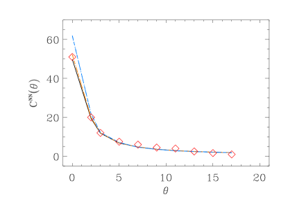
Figure 6: Predicted ACF for the NVSS radio source catalog as a function of angular separation, $\theta$,, in degree. The linear bias factor has been accounted for. The various models correspond, in orange, to $w=-0.9$ and $c_{s}^{2}=0.9,0.1$ (respectively in triple dot-dashed or dot-dashed lines), or, in blue, to $w=-0.3$ with $c_{s}^{2}=0.9,0.1$ (respectively in triple dot-dashed or dot-dashed lines). The black line corresponds to our fiducial $\Lambda$CDM model. Measurements in red are from Nolta03 .

The dimensionless two point correlation function between two quantities $X$ and $Y$ with background values $X_{0}$ and $Y_{0}$ in positions $\hat{n}$ and $\hat{n}^{\prime}$ in the sky is given by

$$C^{XY}(\theta) = \left\langle{\delta X\over X_{0}}(\hat{n}){\delta Y\over Y_{0}}(\hat{n}^{\prime})\right\rangle_{\hat{n}\cdot\hat{n}^{\prime}=cos\theta}$$ (18)

$$= {1\over 4\pi}\sum_{\ell=2}^{\infty}(2l+1)C^{XY}_{\ell}P_{\ell}(cos\theta)$$

For the fractional source count and CMB temperature cross and auto correlations

$$C^{NT}_{\ell} = 4\pi\int_{0}^{\infty}{dk\over k}\left\langle{\delta N\over N_{0}}(k){\delta T\over T_{0}}(k^{\prime})\right\rangle j_{\ell}^{2}(k\eta)$$ (19)

$$= 4\pi\int_{0}^{\infty}{dk\over k}\Delta^{2}(k)f_{\ell}^{N}(k)f_{\ell}^{T}(k)\;,$$

$$C^{NN}_{\ell} = 4\pi\int_{0}^{\infty}{dk\over k}\left\langle{\delta N\over N_{0}}(k){\delta N\over N_{0}}(k^{\prime})\right\rangle j_{\ell}^{2}(k\eta)$$ (20)

$$= 4\pi\int_{0}^{\infty}{dk\over k}\Delta^{2}(k)f_{\ell}^{N}(k)f_{\ell}^{N}(k)\;,$$

where

$$\Delta^{2}(k)=\langle\delta_{c}^{0}(k)\delta_{c}^{0}(k^{\prime})\rangle=\delta(k-k^{\prime})k^{3}P(k)/2\pi^{2}$$ (21)

and where the filter functions for the temperature and number count fluctuations respectively are given by

$$f_{\ell}^{T}(k) = {3H_{0}^{2}\Omega_{m}^{0}\over c^{2}k^{2}}\int^{z}_{0}{dg(z,k)\over dz}j_{\ell}(k\eta(z))dz$$ (22)

$$f_{\ell}^{N}(k) = b_{r}\int_{0}^{z}{d\tilde{N}\over dz}D(z,k)j_{\ell}(k\eta(z))dz\;,$$ (23)

where $D(z,k)$ has been previously defined in section IV.

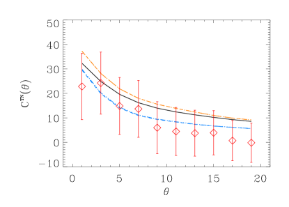
Figure 7: Predicted CCF for the NVSS radio source catalog as a function of angular separation, $\theta$, in degree. The linear bias factor has been accounted for. The various models correspond, in orange, to $w=-0.9$ and $c_{s}^{2}=0.9,0.1$ (respectively in triple dot-dashed, dot-dashed lines), or, in blue, to $w=-0.3$ with $c_{s}^{2}=0.9,0.1$ (respectively in triple dot-dashed or dot-dashed lines). They largely overlap. The black line corresponds to our fiducial $\Lambda$CDM model. Data points from Nolta03 are in red as well as (correlated) error bars.

The results of this approach are summarised in figures 6 and 7. As was used in section IV, we consider here a family of models lying along the CMB angular diameter degeneracy surface, and move along it by varying simultaneoulsy $w$ and $h$. For each of these background, we then consider various $c_{s}^{2}$ and compute the linear transfer function using a modified version of the CMBfast cmbfast or CAMB camb softwares . For a sample of those models, we plotted both the predicted ACF, $C^{NN}(\theta)$, from which we infer the bias (figure 6) and the subsequent predicted CCF, $C^{NT}(\theta)$ which one can compare with the measurements of Nolta03 (figure 7). Obviously, even if this signal does indeed have some dependance with regards to the dark energy pertubations parameters, $w$ and $c_{s}^{2}$, most of the effect is absorbed in the bias measurement illustrated in figure 6. The uncertainty in the bias is the main hindrance in placing constraints on both the equation of state and speed of sound, so that current data do not allow this correlation is not measured well enough to constrain our models. We obtain a bias range and a bias evolution similar as the one obtained by Nolta03 , i.e. $b_{r}\simeq 1.4$ for our fiducial $\Lambda$CDM model, and $b_{r}$ tends to decrease when $w$ increases (in range comprised between 1.4 and 2.2). Note that the plotted error bars are heavily correlated. The knowledge of the correlation matrix computed in Nolta03 allows us however to compute a well defined $\chi^{2}$ statistic. Note also that those error bars include cosmic variance only but do not take into account the shot noise in the radio source catalog. It would be important to consider the uncertainties in the bias measurement that propagates directly in the signal prediction but we leave this issue for future work. Nevertheless, given the fact that all our models lie within the one sigma error bars, we will not illustrate here by a contour plot those weak joint constraints on $w$ and $c_{s}^{2}$.

A natural and important question that arises at this level concerns the future prospect for the measurements of this correlation, depending on the used LSS tracers as well as the survey considered. Although some studies have already been done Hu99 ; Peiris00 ; Cooray02 , more specific investigations are necessary. In particular an independent measurement of the bias, along with improved scale and depth of survey will all contribute to vastly improving on the current observational uncertainties.

VI Conclusions

We have reviewed the effect of the speed of sound of dark energy on CDM and dark energy perturbations. While a positive dark energy speed of sound suppresses the CDM perturbations, it is the deviation from adiabaticity, in combination with the equation of state that determine the degree of suppression of the amplitude dark energy perturbation in comparison to those of the CDM.

We have found the CMB large scale temperature fluctuations, dominated by the ISW effect, are a promising tool to measure the speed of sound. The suppression of CDM matter perturbations drive the late time ISW effect.

From the auto correlation of the WMAP data with itself we obtain a $1\sigma$ ”constraint” on the speed of sound $\hat{c}_{s}^{2}<0.04$, using scenarios that minimise contributions to the likelihood on small scales (from the peaks) as much as possible by using well known degeneracies to follow the WMAP best fit model as closely as possible. The main limitation in obtaining constraints from the auto correlation is the cosmic variance.

We have also investigated the cross correlation of the large scale CMB with fluctuations in the nearby mass distribution using the NVSS radio source catalogue. We here again find that cosmic variance is a strong limitation and prevent us from placing any strong constraint in the $w-c_{s}^{2}$ plane.

However, since the potential of such an analysis might be unique in unveiling the mysteries of the dark energy, it is important to explore further out the prospect of future potential large scale probe of the gravitational portential and so of the ISW (LSST, PLANCK, CMBPOL). We have presented some estimates of prospective constraints that one might obtain from cross correlation of large scale probes with CMB however we leave this exploration for future work.

Acknowledgements We would like to thank Robert Caldwell, Sean Carroll, Anthony Challinor, Rob Crittenden, Joe Hennawi, Mike Nolta, Hiranya Peiris, Martin White and, especially, David Spergel for very helpful discussions and questions in the course of this work. O.D. acknowledges the Aspen Center for Physics where part of this work was pursued. R.B. and O.D. are supported by WMAP and NASA ATP grant NAG5-7154 respectively.

References

- (1) C. L. Bennett et al.astro-ph/0302207
- (2) P.M. Garnavich et al, Ap.J. Letters 493, L53-57 (1998); S. Perlmutter et al, Ap. J. 483, 565 (1997); S. Perlmutter et al (The SupernovaCosmology Project), Nature 391 51 (1998); A.G. Riess et al,Ap. J. 116, 1009 (1998)
- (3) D. N. Spergel et al.astro-ph/0302209
- (4) G. Efstathiou, astro-ph/0303127.
- (5) C.R. Contaldi, M. Peloso, L. Kofman, A. Linde, astro-ph/0303636.
- (6) G. Efstathiou, astro-ph/0306431
- (7) L. A. Kofman & A. A. Starobinskii 1985, Soviet Astronomy Letters, 11, 271
- (8) R.G. Crittenden, N. Turok Phys. Rev. Lett. 76 4 (1996).
- (9) S.P. Boughn, R.G Crittenden astro-ph/0305001
- (10) M.R. Nolta et al.astro-ph/0305097
- (11) P. Fosalba & E. Gatzanaga, astro-ph/0305468
- (12) P. J. E. Peebles, B. Ratra, RMP (2003) in press, astro-ph/0207347.
- (13) J.M. Bardeen, Phys. Rev. D 22 1882 (1980)
- (14) H. Kodama & M. Sasaki, Prog. Theo. Phys. Supp. 78 1 (1984)
- (15) W. Hu, Astrophys. J. 506 485H (1998), astro-ph/9801234
- (16) W. Hu., D. J. Eisenstein, M. Tegmark & M. White 1999, Phys. Rev. D, 59, 23512
- (17) W. Hu,Phys. Rev. D 65 023003 (2002), astro-ph/0108090.
- (18) J. Erikson, R.R. Caldwell, P.J. Steinhardt, V. Mukhanov, and C. Armendariz-Picon Phys. Rev. Lett. 88 121301 (2001)
- (19) S. DeDeo, R.R. Caldwell, P.J. Steinhardt, astro-ph/0301284
- (20) B. A. Bassett, M. Kunz, D. Parkinson, C. Ungarelli, astro-ph/0210640; astro-ph/0211303
- (21) H. Sandvik, M. Tegmark, M. Zaldarriaga, I. Waga, astro-ph/0212144.
- (22) L.M.G. Beca, P.P. Avelino, J.P.M. de Carvalho, C.J.A.P. Martins astro-ph/0303564, to appear in Phys. Rev. D
- (23) R.R.R Reiss, I. Waga, M.O. Calvão, S.E. Jorás astro-ph/0306004.
- (24) R. Bean, O. Doré, Phys. Rev. D in press, astro-ph/0301308
- (25) L. Amendola, F. Finelli, C. Burigana, D. Carturan astro-ph/0304325
- (26) P.G. Ferreira, M. Joyce, Phys. Rev. Lett. 79 4740 (1997); P.G. Ferreira, M. Joyce, Phys. Rev. D 58 023503 (1998)
- (27) G. Gibbons, Phys. Lett. B 537 1 (2002), hep-th/0204008
- (28) A. B. Balakin, D. Pavón, D. Schwarz, W. Zimdahl, astro-ph/0302150
- (29) C.P Ma, E. Bertschinger Astrophys. J. 455 7 (1995).
- (30) E.V. Linder, A. Jenkins astro-ph/0305286
- (31) Verde et al., astro-ph/0302218, Hinshaw et al. astro-ph/0302217; A. Kogut et al., astro-ph/0302213.
- (32) S. Dodelson et al., Astrophys. J. , 572, 140-156 (2001)
- (33) J. Condon et al., Astron. J. 115, 1693 (1998)
- (34) H. Peiris & D. Spergel, Astrophys. J. , 540, 605, 2000
- (35) A. Cooray, A. 2002, Phys. Rev. D, 65, 103510
- (36) S. Boughn, & R. Crittenden, Phys. Rev. Lett. , 88, 21302 (2002)
- (37) S. Boughn, R. Crittenden, & N. Turok 1998, New Astronomy, 3, 275
- (38) S. Boughn, R. Crittenden, & G. P. Koehrsen, Astrophys. J. , 580, 672 (2002)
- (39) J.S. Dunlop, J.A. Peacock MNRAS 247 19 (1990).
- (40) Seljak, U. & Zaldarriaga, M. 1996, Astrophys. J. , 469, 437 , see also http://cmbfast.org/
- (41) http://camb.info/