Bayesian joint analysis of cluster weak lensing and Sunyaev-Zel’dovich effect data

Abstract

As the quality of the available galaxy cluster data improves, the models fitted to these data might be expected to become increasingly complex. Here we present the Bayesian approach to the problem of cluster data modelling: starting from simple, physically motivated parameterised functions to describe the cluster’s gas density, gravitational potential and temperature, we explore the high-dimensional parameter spaces with a Markov-Chain Monte-Carlo sampler, and compute the Bayesian evidence in order to make probabilistic statements about the models tested. In this way sufficiently good data will enable the models to be distinguished, enhancing our astrophysical understanding; in any case the models may be marginalised over in the correct way when estimating global, perhaps cosmological, parameters. In this work we apply this methodology to two sets of simulated interferometric Sunyaev-Zel’dovich effect and gravitational weak lensing data, corresponding to current and next-generation telescopes. We calculate the expected precision on the measurement of the cluster gas fraction from such experiments, and investigate the effect of the primordial CMB fluctuations on their accuracy. We find that data from instruments such as AMI, when combined with wide-field ground-based weak lensing data, should allow both cluster model selection and estimation of gas fractions to a precision of better than 30 percent for a given cluster.

1 Introduction

Clusters of galaxies, as the largest gravitationally bound structures in the Universe, may be used as cosmological probes. The number count of clusters as a function of their mass has been predicted both analytically (see e.g. Press & Schechter, 1974; Sheth et al., 2001) and from large scale numerical simulations (see e.g. Jenkins et al., 2001; Evrard et al., 2002), and are very sensitive to the cosmological parameters $\sigma_{8}$ and $\Omega_{\rm m}$ (Battye & Weller, 2003). The size and formation history of massive clusters is such that the ratio of gas mass to total mass is expected to be representative of the universal ratio $\Omega_{\rm b}/\Omega_{\rm m}$, once the relatively small amount of baryonic matter in the cluster galaxies is taken into account (White et al., 1993).

The deep gravitational potential wells of clusters contain hot ionised gas, which radiates via thermal bremsstrahlung in the X-ray waveband, with a luminosity proportional to the projected squared gas density. Inverse Compton scattering of cosmic microwave background radiation (CMB) photons by this gas produces an observable shift in the thermal spectrum of the CMB in the direction of the cluster (the Sunyaev-Zel’dovich (SZ) effect, Sunyaev & Zeldovich, 1972) which is proportional to the projected gas density. Comparing the SZ and X-ray flux densities allows the angular size distance, and so the Hubble constant, to be measured (Cavaliere, Danese & de Zotti, 1978).

To date, most of our knowledge about clusters has come from optical studies of the cluster member galaxies, and from X-ray observations of the intra-cluster medium. In particular, the recently acquired data from the Chandra and XMM missions have allowed the spatial and spectral features of the X-ray emission from galaxy clusters to be measured in unprecedented detail. This has allowed the measurement of the mass function and global cluster gas fraction to be attempted (Allen et al., 2002; Allen et al., 2003); however, the methodology requires X-ray data from the most massive, relaxed clusters, and includes assumptions of high symmetry and hydrostatic equilibrium.

It is becoming increasingly common to measure the distribution of gas and mass in galaxy clusters by other means. Weakly gravitationally lensed images of field galaxies lying behind the cluster are now routinely observed and used to infer the projected mass distribution of the cluster (see e.g. Kaiser & Squires, 1993; Dahle et al., 2002; Clowe & Schneider, 2002). Similarly, the SZ effect has been observed in many clusters (see e.g. Jones et al., 1993; Carlstrom et al., 1996; Grego et al., 2001), and has been used with some success in the determination of H₀ (see e.g. Birkinshaw & Hughes, 1994; Jones et al., 2001; Mason et al., 2001; Grainge et al., 2002; Reese et al., 2002). Clearly a more complete analysis of clusters of galaxies utilising all these data at the same time would be desirable. In this paper we outline our general approach to this task, and show how our methods give natural answers to the specific questions being asked of the data. Either Hubble’s parameter, or the cluster gas fraction, or indeed both, could equally well be chosen as the cosmological parameter for the demonstrative purposes of this work; for simplicity we focus on the gas fraction, setting H${}_{0}=100h\;\textrm{km s}^{-1}$.

The quality of X-ray data in the past, and that of current weak lensing and SZ data, is such that the information content of each dataset individually matches that of a simple, symmetric, constrained model, with just a handful of parameters. One might expect that combining the datasets would lead to an improvement in the parameter estimates, and thus open up the possibility of testing more complex models. In this work we simulate and compare observations made with current generation SZ telescopes, such as the VSA (Watson et al. 2003) and CBI (Pearson et al. 2003), with those under construction such as AMI (Kneissl et al. 2001) and the SZA (Mohr et al. 2002). In each case we match the mock SZ observations with simulated wide field lensing data, and investigate the prospects for measuring the cluster gas fraction via this route.

In Section 2 we discuss a systematic approach to the problem of cluster model parameter fitting and model selection. We also show in this context how to infer model-independent conclusions from cluster data, where the derived errors on, in particular, any inferred cosmological parameters take the uncertainty in the cluster model into account. After an introduction to the example cluster data and models in Sections 3 and 4, we apply these methods to simulated sets of data from weak gravitational lensing and the SZ effect observed by microwave interferometers in Section 5, and discuss the prospects of the aforementioned current and near-future experiments. We then put the results of this demonstration in context with a brief discussion of our methodology and others (Section 6), and summarise our conclusions in Section 7.

2 Bayesian inference

For a set of data arranged into a vector $\mathbf{d}$, our knowledge of the experimental errors on those data can be written in the form of a likelihood function $L$:

$$L=\textrm{Pr}(\mathbf{d}|\mn@boldsymbol{\theta},\mathnormal{H}_{j}),$$ (1)

which is a function of the observed data and depends on the parameter vector $\mn@boldsymbol{\theta}$ of an assumed model or hypothesis $\mathnormal{H}_{j}$. By the central limit theorem the likelihood can often be approximated by a multivariate Gaussian,

$$L=\frac{1}{|2\pi\mathsf{C}|^{\frac{1}{2}}}\exp{-\frac{1}{2}(\mathbf{d}-\mathbf{d}_{p})^{T}\mathsf{C}^{-1}(\mathbf{d}-\mathbf{d}_{p})}$$ (2)

where the predicted data vector $\mathbf{d}_{p}$ is calculated within the model $\mathnormal{H}_{j}$. However, other forms of the likelihood function may describe the data more accurately; none of the rest of this section relies on the Gaussian approximation. If the data vector can be written as

$$\mathbf{d}=\mathbf{d}_{1}+\mathbf{d}_{2},$$ (3)

where the two sub-datasets are independent, then we can write the joint likelihood as

$$\textrm{Pr}(\mathbf{d}|\mn@boldsymbol{\theta},\mathnormal{H}_{j})=\textrm{Pr}(\mathbf{d}_{1}|\mn@boldsymbol{\theta},\mathnormal{H}_{j})\textrm{Pr}(\mathbf{d}_{2}|\mn@boldsymbol{\theta},\mathnormal{H}_{j}),$$ (4)

as has been applied to cluster potential analysis by Castander et al. (2000).

At this point we can ask the following questions:

1. “What are the relative probabilities of any two models $\mathnormal{H}_{i}$ and $\mathnormal{H}_{j}$ being the true model, given all the information we have?”

2. “What is the joint probability distribution of the parameters $\mn@boldsymbol{\theta}$ of model $\mathnormal{H}_{i}$, given all the information we have?”

3. “What is the probability distribution of any one particularly interesting parameter $\theta_{k}$, given all the information we have?”

In the context of galaxy cluster data analysis, a model will be a set of suitably parameterised functions describing the cluster potential, gas density and temperature, and a suitably parameterised background cosmology; all of these parameters are included in the vector $\mn@boldsymbol{\theta}$ and should be inferred simultaneously. Learning the structure of the cluster involves finding the most appropriate cluster model and its parameters; the first two questions above can therefore be bracketed together as “astrophysical” questions. To do cosmology with clusters one just wants to investigate the cosmological part of the parameter space, in a way that is independent of the cluster model. In this respect, question (iii) can be labelled “cosmological”.

2.1 Model selection and parameter fitting: astrophysics

The answer to question (ii) above is given by Bayes’ theorem:

$$\textrm{Pr}(\mn@boldsymbol{\theta}|\mathbf{d},\mathnormal{H}_{j})=\frac{\textrm{Pr}(\mathbf{d}|\mn@boldsymbol{\theta},\mathnormal{H}_{j})\textrm{Pr}(\mn@boldsymbol{\theta}|\mathnormal{H}_{j})}{\textrm{Pr}(\mathbf{d}|\mathnormal{H}_{j})}.$$ (5)

The probability density function (pdf) $\textrm{Pr}(\mn@boldsymbol{\theta}|\mathnormal{H}_{j})$ should encode any prior knowledge we have of the parameters of the model in question. For example, uncertainty as to the order of magnitude of a parameter should be represented by a uniform probability distribution in the logarithm of the parameter (Jeffreys, 1932), whilst a previously performed, independent measurement of a parameter might be interpreted as a Gaussian prior centred on the observed value with width equal to the quoted error.

The denominator of equation (5) plays an important role in answering question (i). Applying Bayes’ theorem again we have

$$\textrm{Pr}(\mathnormal{H}_{j}|\mathbf{d})=\frac{\textrm{Pr}(\mathbf{d}|\mathnormal{H}_{j})\textrm{Pr}(\mathnormal{H}_{j})}{\textrm{Pr}(\mathbf{d})}.$$ (6)

Here, the denominator is a constant. Moreover, if, prior to the analysis, the various models are assigned equal probabilities (as might be the case for an attempt at a “fair test”, or if the analyst really does have no more belief in any one model than another), then the quantity $\textrm{Pr}(\mathbf{d}|\mathnormal{H}_{j})$ may be used in comparing the relative probailities of each model under consideration. For more details on the use of this quantity, known as the “evidence” (see e.g. Jaynes, 2003; MacKay, 1992). Calculation of the evidence is in principle straightforward; marginalising out the $N_{i}$ parameters of the model gives

$$\textrm{Pr}(\mathbf{d}|\mathnormal{H}_{j})=\int\textrm{Pr}(\mathbf{d}|\mn@boldsymbol{\theta},\mathnormal{H}_{j})\textrm{Pr}(\mn@boldsymbol{\theta}|\mathnormal{H}_{j})\,d^{N_{i}}\mn@boldsymbol{\theta}.$$ (7)

However, for the purposes of this work it is useful to note that the evidence is sensitive both to the parameter prior and the likelihood. Models providing a better fit to the data, and so a higher value at the peak of the likelihood function, have higher evidence associated with them. Conversely, models whose priors define large volumes of low likelihood parameter space will give lower evidence values – overly complex models are penalised.

We now turn to the practical problems associated with the calculation of the posterior probability $\textrm{Pr}(\mn@boldsymbol{\theta}|\mathbf{d},\mathnormal{H}_{j})$ and the associated evidence $\textrm{Pr}(\mathbf{d}|\mathnormal{H}_{j})$. One approach, much used in the field of cosmological parameter estimation, is to calculate the prior density and likelihood on a discrete parameter grid. However, as the models considered become more complex, this task becomes exponentially more computationally intensive. As an illustration, if a likelihood evaluation for a 10 parameter model takes just 1 second, the time to produce a grid of posterior probability densities, ten pixels in each dimension, is of order $10^{10}$ seconds, or 300 years. Clearly this procedure is neither practical nor accurate. Instead, we use an exploratory Markov-Chain Monte-Carlo (MCMC) algorithm to draw samples from the multidimensional unnormalised posterior $\textrm{Pr}(\mathbf{d}|\mn@boldsymbol{\theta},\mathnormal{H}_{j})\textrm{Pr}(\mn@boldsymbol{\theta}|\mathnormal{H}_{j})$ (Gilks et al., 1996). The output of the MCMC algorithm is a list of samples whose number density in parameter space is proportional to the posterior probability density. This allows a representation of the desired posterior to be constructed which is both efficiently calculated (computation time is typically of the order of a few hours) and convenient to use. For example, the sample parameter values may be combined to calculate predictions for other properties of the model.

Calculating the evidence by performing the integral of equation (7) numerically by ordinary means would of course involve a similar number of operations as that outlined above. We instead make use of the technique of “thermodynamic integration” to calculate the evidence dynamically during an initial “burn-in” phase of the MCMC algorithm (Gilks et al., 1996). This process results in evidence values precise to a fraction of a unit in $\log_{e}{\textrm{Pr}(\mathbf{d}|\mathnormal{H}_{j})}$. This corresponds to a probability ratio between two models’ of less than 3, well below the “belief threshold” of a sensible analyst.

2.2 Marginalising over parameters and models: cosmology

A major benefit of working with samples drawn from the posterior rather than a grid of posterior values is that the process of marginalisation becomes trivial. When estimating a single parameter $\theta_{i}$ of a model $\mathnormal{H}_{j}$ the distribution of interest is

$$\textrm{Pr}(\theta_{i}|\mathbf{d},\mathnormal{H}_{j})=\int\textrm{Pr}(\mn@boldsymbol{\theta}|\mathbf{d},\mathnormal{H}_{j})\,d^{{N_{i}}-1}\mn@boldsymbol{\theta},$$ (8)

where the integral is over all other parameters. This projection takes into account all the parameter degeneracies of the model, as well as the priors on all of the parameters. An ensemble of sample $\mn@boldsymbol{\theta}$-vectors drawn from the full posterior can be projected onto the $\theta_{i}$ direction just by extracting the $\theta_{i}$ values from the ensemble.

Although computing $n$-point statistics from a set of samples is very easy, reconstructing the marginalised posterior pdf is not so straightforward. To do this we provide as estimators for these distributions histograms of sample values smoothed to some arbitrary length scale, such that we err on the side of caution and never underestimate the distribution widths. This is in keeping with our general approach: the marginalised posterior probability distribution $\textrm{Pr}(\theta_{k}|\mathbf{d})$ is in general broader than those conditional on other parameters being fixed at, for instance, the maximum likelihood point. The resulting estimators are therefore as accurate as possible, since the maximum amount of information has been included, and as precise as allowed by the quality of the data, since the errors on the observed quantities have been rigorously propagated in a self-consistent way.

By taking this process one step further we can answer question (iii), by marginalising over model space. This procedure is important in the context of cluster data analysis: we want to be able to make robust, model-independent statements about cosmological parameters from cluster data. To this end, and denoting the cosmological parameter of interest $\theta_{k}$, one should calculate

$$\textrm{Pr}(\theta_{k}|\mathbf{d}) =\underset{j}{\sum}\textrm{Pr}(\theta_{k}|\mathbf{d},\mathnormal{H}_{j})\textrm{Pr}(\mathnormal{H}_{j}|\mathbf{d})$$ (9)

$$\propto\underset{j}{\sum}\textrm{Pr}(\theta_{k}|\mathbf{d},\mathnormal{H}_{j})\textrm{Pr}(\mathbf{d}|\mathnormal{H}_{j})\textrm{Pr}(\mathnormal{H}_{j}).$$ (10)

The last proportionality is as such because we have discarded the normalising constant of equation (6). Equation (10) is now a relationship between quantities that we can calculate, and represents a model-averaging process. We might hope that one particular model would be many times more probable given the data, in which case we have learnt something about the astrophysics of the cluster and the sum will be dominated by this model. On the other hand, it is always possible to construct a range of models whose parameter priors all match the data’s likelihood equally well, and so give similar evidences. In this case the averaging process serves to increase the width of the posterior density of interest, that of the interesting parameter $\theta_{k}$ given the data only, by an amount appropriate to the uncertainty over the range of models. In this way, (quasi)-model independent statements can be made about cosmological parameters, such as the cluster gas fraction, from the cluster data.

3 Data

In this section we give a brief introduction to weak lensing and interferometric Sunyaev-Zel’dovich effect data, demonstrating the construction of the likelihood function in each case.

3.1 Weak lensing

Weak gravitational lensing may be used to investigate cluster mass distributions through the relationship (see e.g. Schramm & Kayser, 1995)

$$\langle\epsilon\rangle=g(\mn@boldsymbol{\theta});$$ (11)

that is, the average complex ellipticity $\epsilon=\epsilon_{1}+i\epsilon_{2}$ of an ensemble of background galaxy images is an unbiased estimator of the local reduced shear field ($g$) due to the cluster. Equation (11) allows us to use each of the $2N_{\rm gal}$ lensed ellipticity components $\epsilon_{j}$ of $N_{\rm gal}$ measured background galaxy images as noisy estimators for the corresponding component of the reduced shear $g_{j}(\mn@boldsymbol{\theta})$ due to the cluster model, parameterised with the variables $\mn@boldsymbol{\theta}$ (Seitz et al., 1998; Schneider et al., 2000; Marshall et al., 2002).

Here, the complex ellipticity is defined such that an elliptical object with semi-major axis $a$, semi-minor axis $b$ and orientation angle (measured anticlockwise from $x$-axis to semi-major axis) $\phi$ has ellipticity

$$\epsilon=\frac{a-b}{a+b}e^{2i\phi}.$$ (12)

Figure 1 of Kaiser et al. (1995) shows the image shapes corresponding to different values of this (or a similarly defined) ellipticity; the effect of an isolated mass concentration lying in front of a galaxy field is to align the image shapes tangentially about the centre of the mass distribution. Large catalogues of background galaxies with measured ellipticities are now almost routinely generated from wide field optical images, using shape estimation software such as imcat (Kaiser et al., 1995) or im2shape (Bridle et al., 2001).

We may organise the observed ellipticities into the data vector $\mathbf{d}$, having components

$$\mathnormal{d}_{i}=\left\{\begin{array}[]{ll}\textrm{Re}(\epsilon_{i})&\mbox{$\left(i\leq N_{\rm gal}\right)$}\\ &\\ \textrm{Im}(\epsilon_{i-N_{\rm gal}})&\mbox{$\left(N_{\rm gal}+1\leq i\leq 2N_{\rm gal}\right)$}\end{array}\right..$$ (13)

Likewise the corresponding model reduced shears can be arranged into the predicted data vector $\mathbf{d}^{\rm p}$, having components

$$\mathnormal{d}^{\rm p}_{i}=\left\{\begin{array}[]{ll}\textrm{Re}(g_{i})&\mbox{$\left(i\leq N_{\rm gal}\right)$}\\ &\\ \textrm{Im}(g_{i-N_{\rm gal}})&\mbox{$\left(N_{\rm gal}+1\leq i\leq 2N_{\rm gal}\right)$}\end{array}\right..$$ (14)

The unlensed ellipticity components may often be taken as having been drawn independently from a Gaussian distribution with mean $g_{j}$ and variance $\sigma_{\rm intrinsic}^{2}$, leading to a diagonal noise covariance matrix $\mathsf{C}$. We can then write the likelihood function as

$$L_{\rm Lensing} =\textrm{Pr}(\mbox{\mbox{Data}}|\mn@boldsymbol{\theta})$$ (15)

$$=\frac{1}{Z_{L}}\exp(-\frac{\chi^{2}}{2}),$$

where $\chi^{2}$ is the usual misfit statistic

$$\chi^{2} =\sum_{i=1}^{N_{\rm gal}}\sum_{j=1}^{2}\frac{\left(\epsilon_{j,i}-g_{j,i}(\mn@boldsymbol{\theta})\right)^{2}}{\sigma^{2}}$$ (16)

$$=\left(\mathbf{d}-\mathbf{d}^{\rm p}\right)^{\rm T}\mathsf{C}^{-1}\left(\mathbf{d}-\mathbf{d}^{\rm p}\right),$$ (17)

and the normalisation factor is

$$Z_{L}=(2\pi)^{2N_{\rm gal}/2}|\mathsf{C}|^{1/2}.$$ (18)

The effect of Gaussian errors introduced by the galaxy shape estimation procedure has been included by adding them in quadrature to the intrinsic ellipticity dispersion (Hoekstra et al., 2000; Marshall et al., 2002),

$$\sigma=\sqrt{\sigma^{2}_{\rm obs}+\sigma^{2}_{\rm intrinsic}}.$$ (19)

This approximation includes the assumption that the applied reduced shear is not too large (as is the case for low redshift clusters).

3.2 Sunyaev Zel’dovich effect

To date, the majority of the observations of the SZ effect towards clusters of galaxies have been made with interferometers (see e.g. Joy et al., 2001; Jones et al., 2001; LaRoque et al., 2003). These instruments have a number of advantages over single dish telescopes, including their relative insensitivity to atmospheric emission (e.g. Lay & Halverson, 2000), lack of required receiver stability, and the ease with which systematic errors such as ground spill (Watson et al. 2003) and point source contamination (Grainger et al. 2002, Taylor et al. 2003) can be minimised.

Assuming a small field size, an interferometer operating at a single frequency $\nu$ measures samples from the complex visibility plane $\widetilde{I}_{\nu}(\mn@boldsymbol{u})$. This is given by the weighted Fourier transform of the surface brightness $I_{\nu}$,

$$\widetilde{I}_{\nu}(\mn@boldsymbol{u})=\int A_{\nu}(\mn@boldsymbol{x})I_{\nu}(\mn@boldsymbol{x})\exp(2\pi i\mn@boldsymbol{u}\cdot\mn@boldsymbol{x})~{}{\rm d}^{2}\mn@boldsymbol{x},$$ (20)

where $\mn@boldsymbol{x}$ is the position relative to the phase centre, $A(\mn@boldsymbol{x},\nu)$ is the (power) primary beam of the antennas at the observing frequency $\nu$ (normalised to unity at its peak), and $\mn@boldsymbol{u}$ is a baseline vector in units of wavelength.

The positions in the $uv$-plane at which this function is sampled by the interferometer are determined by the physical positions of its antennas and the direction of the field on the sky. The samples $\mn@boldsymbol{u}_{j}$ lie on a series of curves which we may denote by the function $\widetilde{B_{\nu}}(\mn@boldsymbol{u})$ that equals unity where the Fourier domain (or $uv$-plane) is sampled and equals zero elsewhere. The function $\widetilde{B_{\nu}}(\mn@boldsymbol{u})$ may be inverse Fourier transformed to give the synthesised beam $B_{\nu}(\mn@boldsymbol{x})$ of the interferometer at an observing frequency $\nu$.

For a realistic interferometer, the sample values will also contain a contribution due to noise; the $j$th baseline $\mn@boldsymbol{u}_{j}$ of an interferometer measures the complex visibility

$$V(\mn@boldsymbol{u}_{j})=\widetilde{I}_{\nu}(\mn@boldsymbol{u}_{j})+N(\mn@boldsymbol{u}_{j}),$$ (21)

where $N(\mn@boldsymbol{u}_{j})$ is the noise on the $j$th visibility. This noise comes from two sources: the first is uncorrelated Johnson noise from the receivers. The second source of noise is the CMB itself, now known to be very well approximated by a Gaussian random field defined by its angular power spectrum. That is, expanding the primordial CMB surface brightness distribution into a spherical harmonic series gives

$$I_{\nu}^{\rm CMB}=\sum_{\ell=0}^{\infty}\sum_{m=-\ell}^{\ell}a_{\ell m}(\nu)Y_{\ell m}(\hat{\mn@boldsymbol{x}}),$$ (22)

leading to the power spectrum

$$c_{\ell}=\langle|a_{\ell m}|^{2}\rangle.$$ (23)

For small fields of view, the index $\ell$ is related to the Fourier ($uv$) plane vector  $\mn@boldsymbol{u}$ by $\ell\approx 2\pi|\mn@boldsymbol{u}|$. An ideal interferometer would therefore measure the $a_{\ell m}$ directly, giving an extra noise vector

$$N^{\rm CMB}(|\mn@boldsymbol{u}|)=\sqrt{c}_{\ell}.$$ (24)

In practice, the interferometer observes the sky surface brightness multiplied by the primary beam $A_{\nu}(\mn@boldsymbol{x})$; the corresponding convolution with the aperture illumination function $\widetilde{A}_{\nu}(\mn@boldsymbol{u})$ in the $uv$-plane produces correlated visibilities. Since the SZ effect produces a (frequency dependent) linear perturbation $\delta I_{\nu}$ to the CMB surface brightness, the noise on an SZ observation can therefore be described by the covariance matrix

$$\mathsf{C}=\mathsf{C}^{\rm receiver}+\mathsf{C}^{\rm CMB}.$$ (25)

The first term on the right hand side is a diagonal matrix with elements $\sigma^{2}_{i}\delta_{ij}$, with $\sigma_{i}$ the rms Johnson noise on the $i^{th}$ baseline visibility. The second term contains significant off-diagonal elements and can be calculated from a given primordial CMB power spectrum following Hobson & Maisinger (2002). Rather than dealing with complex data and covariance matrices, it is convenient to order the visibility components into a data vector $\mathbf{d}$ with components

$$\mathnormal{d}_{i}=\left\{\begin{array}[]{ll}\textrm{Re}(V_{i})&\mbox{$\left(i\leq N_{\rm vis}\right)$}\\ &\\ \textrm{Im}(V_{i-N_{\rm vis}})&\mbox{$\left(N_{\rm vis}+1\leq i\leq 2N_{\rm vis}\right)$}\end{array}\right..$$ (26)

With an inversionally symmetric primary beam pattern there is no correlation between the real and imaginary parts of the visibilities, so with this ordering of the data the matrix $\mathsf{C}^{\rm CMB}$ is block-diagonal. The power spectrum is often approximated to be constant within each of a set of bins in the spherical harmonic coefficient index $l$; these bins therefore correspond to annuli in the $uv$-plane, and the “flat band powers” $d_{b}=\langle\ell(\ell+1)c_{\ell}\rangle_{b}$ are then related to the CMB covariance matrix by an equation of the form

$$\mathsf{C}^{\rm CMB}_{\mathnormal{ij}}=\sum_{b}d_{b}J_{\mathnormal{ij}}(|\mn@boldsymbol{u}|_{b},|\mn@boldsymbol{u}|_{b+1}),$$ (27)

where the $b^{th}$ bin covers the range $|\mn@boldsymbol{u}|_{b}$ to $|\mn@boldsymbol{u}|_{b+1}$, and the integrals $J_{ij}$ take the effect of the the aperture illumination function into account. Figure 1 shows the power spectrum used in the generation of the covariance matrix $\mathsf{C}^{\rm CMB}$ for simulated VSA data.

Figure 1: The flat band powers used to create the covariance matrix associated with the primary CMB fluctuations on the sky. The dotted lines correspond roughly to the range of scales that can be probed by the VSA in its present extended configuration. Overplotted is a theoretical model corresponding to the flat $\Lambda$CDM model favoured by the WMAP satellite data.

With the combined covariance matrix $\mathsf{C}$ in hand, the likelihood function can be written

$$L_{\rm SZ} =\textrm{Pr}(\mbox{\mbox{Data}}|\mn@boldsymbol{\theta})$$ (28)

$$=\frac{1}{Z_{L}}\exp\left(-\frac{\chi^{2}}{2}\right),$$

where $\chi^{2}$ is again a statistic quantifying the misfit between observed data $\mathbf{d}$ and predicted data $\mathbf{d}^{p}$, the latter of which is a function of the model SZ surface brightness $\delta I_{\nu}$:

$$\chi^{2}=\left(\mathbf{d}-\mathbf{d}^{\rm p}\right)^{\rm T}\mathsf{C}^{-1}\left(\mathbf{d}-\mathbf{d}^{\rm p}\right),$$ (29)

and the normalisation factor is

$$Z_{L}=\left(2\pi\right)^{2N_{\rm vis}/2}|\mathsf{C}|^{1/2}.$$ (30)

3.3 Joint analysis

As given in equation (3), the independent likelihoods described in the previous subsections can be simply combined to give the joint likelihood

$$\log{L}=\log{L_{\rm SZ}}+\log{L_{\rm Lensing}}.$$ (31)

If the datasets contain systematic errors, then some attempt to deal with this can be made by applying hyperparameters to the likelihoods (Lahav et al., 2000; Hobson et al., 2002); this further complication is not considered here. It is sufficient to note that such a mismatch between the conclusions drawn independently from the two datasets should result in a joint log evidence smaller than the sum of the two individual log evidence values.

4 Simple cluster models

Clearly the sum over models in equation (10) can be simplified by discarding the terms with neglible weight; this corresponds to investigating only physically reasonable models, starting with the simplest and gradually increasing the complexity as required by the data via the evidence. With this in mind, and for the illustrative purpose of this work we limit ourselves to investigating just two cluster models, referred to as “Beta” and “iHSE”.

Both models are spherically symmetric, with centroids assumed to be known to within a Gaussian error of $\pm 1$ arcmin. All projected distributions are then circularly symmetric, with profiles defined as a function of projected radius $s=\sqrt{(x-x_{0})^{2}+(y-y_{0})^{2}}$. The three distributions taken to be fundamental in defining the cluster model are taken to be the gravitational potential due to the total mass density (including dark matter and intracluster medium), the density of hot gas in the cluster, and the gas temperature.

4.1 Mass distributions

For simplicity, we limit ourselves in this work to a single model for the mass distribution, and choose for this purpose the NFW profile (Navarro, Frenk & White, 1995). This has been found to provide a good fit to many numerically simulated clusters, and is simple enough that analytic formulae for many derived distributions have been worked out, as described below. The three-dimensional radial dependence of the density is given by

$$\rho(r)=\frac{\rho_{s}}{\left(r/r_{s}\right)\left(1+r/r_{s}\right)^{2}}.$$ (32)

The gravitational lensing data are sensitive only to the projected total mass density distribution, $\Sigma(x)$, where $x$ is the scaled projected radius $x=s/r_{s}$. For a circularly symmetric surface density, the magnitude of the shear is given by

$$|\gamma|=\frac{\overline{\Sigma}(x)-\Sigma(x)}{\Sigma_{\rm crit}}$$ (33)

(with the overbar denoting average density within $x$). Here, the critical density $\Sigma_{\rm crit}$ is a factor dependent on the angular diameter distances to and between the lens ($l$) and source ($s$) planes:

$$\Sigma_{\rm crit}=\frac{c^{2}}{4\pi G}\frac{D_{s}}{D_{l}D_{ls}}.$$ (34)

The complex reduced shear at background galaxy position radius $x$ and azimuthal angle $\phi$ can then be formed from

$$g=\frac{|\gamma|(x)}{1-\kappa(x)}\left(-\cos(2\phi)-i\sin(2\phi)\right),$$ (35)

(with the convergence $\kappa=\Sigma/\Sigma_{\rm crit}$) and provide the predicted lensing data. Analytical formulae for $|\gamma|(x)$ and $\kappa(x)$ are given by Wright & Brainerd (2000) and are not reproduced here.

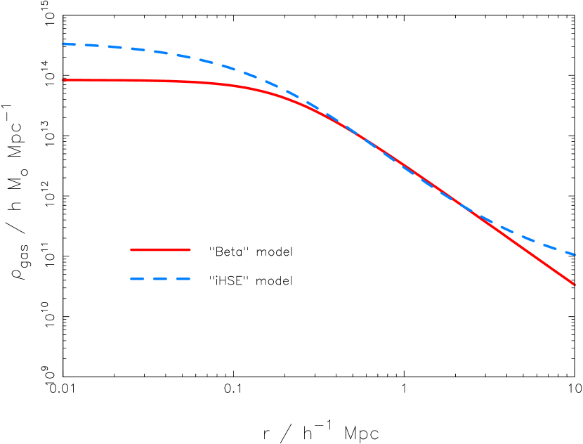
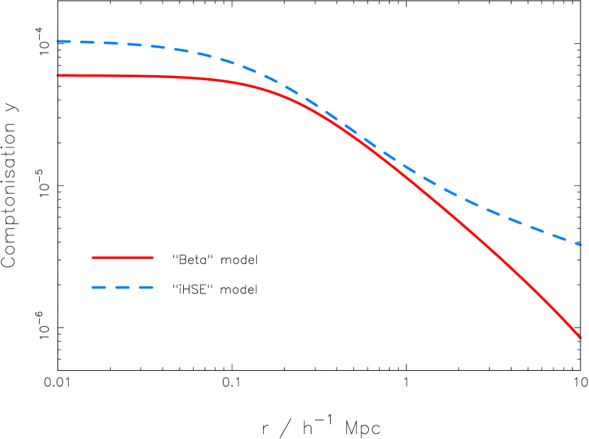
Figure 2: Deprojected radial gas density (left), and Comptonisation parameter $y$ (right) for the two simulated clusters described in the text.

Note that for the NFW model the predicted lensing data are most easily parameterised in terms of a scale radius and density; however, the prior which we understand best is on the total mass, defined to be that within a radius $r_{200}$ such that the average density within $r_{200}$ is 200 times the critical density of the Universe. The overdensity 200 is a value often used by workers investigating numerical simulations of clusters, a potential source of prior information. Given values of $M_{200}$ and the corresponding concentration parameter $c_{200}=r_{200}/r_{s}$, the scale radius and density can be computed.

4.2 Gas distributions

The SZ data are sensitive only to the cluster gas pressure, which must be calculated from the model gas density and temperature distributions. Both models assume a one-parameter isothermal temperature profile. The difference between the models comes in the gas density distribution. The Beta model has gas density profile

$$\rho_{\rm gas}(r)=\frac{\rho_{\rm gas}(0)}{\left(1+\left(r/r_{c}\right)^{2}\right)^{\frac{3\beta}{2}}},$$ (36)

often used in cluster modelling (see e.g. Sarazin, 1988). In the iHSE model the gas is in full hydrostatic pressure equilibrium with the potential defined by the NFW mass model (iHSE). This potential is

$$\Phi =-\frac{GM(r)}{r}$$ (37)

$$=-\frac{4\pi G\rho_{s}r_{s}^{3}}{r}\left[\log(1+r/r_{s})-\frac{r/r_{s}}{1+r/r_{s}}\right].$$ (38)

The equation of hydrostatic equilibrium is

$$\nabla P=-\rho_{\rm gas}\nabla\Phi,$$ (39)

which, with the assumption of a spherically symmetric distribution of ideal gas at temperature $T$, becomes

$$\frac{d\log{\rho_{\rm gas}}}{d\log{r}}=-\frac{GM(r)\mu}{kTr}.$$ (40)

We assume a mass per particle of $\mu=0.59$ times the proton mass. Given the potential of equation (38), this equation can be integrated (Suto et al., 1998) to give

$$\rho_{\rm gas}=\rho_{\rm gas}(0)\exp{-\frac{4\pi G\rho_{s}r_{s}^{2}\mu}{kT}\left(1-\frac{\log(1+r/r_{s})}{r/r_{s}}\right)}$$ (41)

Note again that the predicted data are most easily expressed in terms of a central gas density $\rho_{gas}(0)$, which can be computed by numerically integrating either gas density profile to $r_{200}$ and normalising to the gas mass within this radius, a parameter for which again the prior is better understood. This integral is performed numerically, as is the Abel integral used in projecting the gas pressure distribution along the line of sight $l$, as required in the calculation of the Compton $y$-parameter:

$$y(s) =\frac{\sigma_{\rm T}}{m_{e}c^{2}}\int_{-\infty}^{\infty}n_{e}kTdl$$ (42)

$$\propto\int_{s}^{\infty}\frac{2r\rho_{\rm gas}(r)}{\sqrt{r^{2}-s^{2}}}dr.$$ (43)

Predicted visibilities are generated by sampling the (Fast) Fourier transform of the 30 GHz sky surface brightness $\delta I_{\nu}$, related to the $y$-parameter by

$$\delta I_{\nu}=f(\nu)yB_{\nu}(T_{\rm CMB}),$$ (44)

where $B_{\nu}(T_{\rm CMB})$ is the CMB blackbody spectrum and $f(\nu)$ is a frequency-dependent factor approximately equal to $-2$ at 30 GHz.

Figure 2 shows the Beta and iHSE model profiles, as functions of three-dimensional radius for the gas density profile (equation (41)), and of projected radius for the Comptonisation parameter (equation (43)). Finally, the reader should note that the Beta profile, free from the hydrostatic equilibrium constraint, has two extra parameters, making it more flexible in fitting the data. Moreover, the two gas density profiles described here have been chosen to have the same method of normalisation, allowing straightforward comparison of the two models in fitting the data. This is purely a matter of convenience, and is not required by the methodology of Section 2.

5 Application to simulated data

Table 1: Cluster model parameters and priors. Inequalities denote uniform prior probability between the given limits, whilst $(a\pm b)$ indicates a Gaussian prior centred on $a$ with variance $b^{2}$.

Dataset	Model	Parameters	Truth	Priors
Both		$x_{0},y_{0}$	0.0,0.0	$(0\pm 1)$ arcmin
Gravitational	Both	$M_{200}$	$7.0\times 10^{14}h^{-1}\textrm{M}_{\odot}$	$0<M_{200}/h^{-1}\textrm{M}_{\odot}<2\times 10^{15}$
lensing		$c_{200}$	4	$0<c_{200}<12$
SZ effect	Both	$M_{\rm gas}$	$4.9\times 10^{13}h^{-2}\textrm{M}_{\odot}$	$0<M_{\rm gas}/h^{-2}\textrm{M}_{\odot}<3\times 10^{14}$
		$T$	8 keV	$(8\pm 2)$ keV
	Beta	$r_{c}$	$200h^{-1}$ kpc	$0<r_{c}/h^{-1}\textrm{kpc}<1000$
	only	$\beta$	0.667	$0.3<\beta<1.5$

In this section we use simulated data to demonstrate the methods outlined in Section 2. We first focus on simulations of current data, namely observations of low redshift clusters in the optical with MegaCam at CFHT (Marshall et al. 2003 in preparation), and at 30 GHz with the extended VSA (Lancaster et al. 2003 in preparation). We then move on to consider data of the quality we might expect in the near future, at higher redshift with SZ telescopes such as AMI. This is considered in combination with ground-based lensing data from a camera with field of view again well-matched to the SZ observations.

Our strategy is to simulate lensing and SZ data using each of the model clusters described in the previous section, and then analyse these data as recommended in Section 2, assuming in turn both of the models (one of which is the correct one). The “true” cluster parameters for each model are given in Table 1. We use the same model clusters for both current and next-generation mock observations, the only difference being a shift in redshift from 0.07 (current observations) to 0.2 (next-generation observations). Also given in Table 1 are the prior pdfs used in the mock analyses. The profiles plotted in Figure 2 correspond to these choices of true parameters.

The lensing data were generated by drawing $N$ background galaxy ellipticities from a Gaussian intrinsic ellipticity distribution of width 0.25, lensing them by the calculated reduced shear field of the cluster, then adding realistic Gaussian shape measurement noise with $\sigma_{\rm obs}=0.2$. $N$ was specified by choosing a source density of 15 arcmin^-2, appropriate to a 3-hour ground-based observation (Clowe & Schneider, 2002).

For the mock SZ datasets, the Fourier transform of the model cluster’s surface brightness was calculated at each of the telescope-sampled points in the $uv$-plane; Gaussian noise was then added, drawn from the covariance matrix described in Section 3.2 with thermal receiver noise corresponding to 150 hours’ observation.

5.1 Measuring cluster gas fractions

With the model gas and total mass density profiles both normalised to the respective mass within $r_{200}$, it is straightforward to compute the cluster gas fraction within the same radius. Since the observable quantities, the Comptonisation parameter $y$ and the reduced shear $g$, cannot depend on the Hubble constant, the gas mass must have units of $h^{-2}\textrm{M}_{\odot}$ while the units of total mass are $h^{-1}\textrm{M}_{\odot}$. Consequently, the gas fraction measurable by combination of weak lensing and SZ effect data contains a factor of $h$:

$$\frac{M_{\rm gas}}{M_{200}}=f_{\rm gas}h.$$ (45)

This is the same $h$-dependence as found by Grego et al. (2001) when constraining the potential with the assumption of hydrostatic equilibrium, but is different from that arising from the fitting of X-ray data. Combination of the results from lensing and SZ data with those from an analysis of X-ray data will thus break the degeneracy between the gas fraction and the Hubble parameter; this combination may be done equivalently by simultaneously fitting all three data sets simultaneously, or by applying the joint posterior pdf from the X-ray analysis as a prior for the SZ/lensing analysis, or vice versa.

Figure 3: Implied prior probability distribution $\textrm{Pr}(f_{\rm gas}h)$, as represented by an unsmoothed histogram of 50000 MCMC samples.

In this work, we leave the $h$-dependence of the gas fraction as it is, simply using the uniform priors of Table 1 on $M_{\rm gas}$ and $M_{200}$. However, these apparently innocuous priors lead to an informative prior on the combination $f_{\rm gas}h$. This can be seen by sampling the joint prior with no data using the MCMC algorithm (Slosar et al. 2003), and computing $M_{\rm gas}/M_{200}$ for each sample in the same way as would be done in the data analysis process. The resulting histogram is shown in Figure 3. The effect of the upper limit on the gas mass can be seen as the turnover point at $M_{\rm gas,max}/M_{200,max}=0.15$. Below this value, the prior is uniform, whereas above it the larger values of $f_{\rm gas}h$ are increasingly disfavoured, well reflecting our prior knowledge of cluster masses.

5.2 Current generation experiments

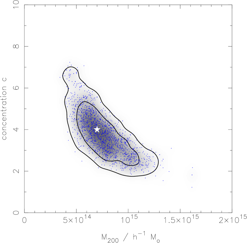
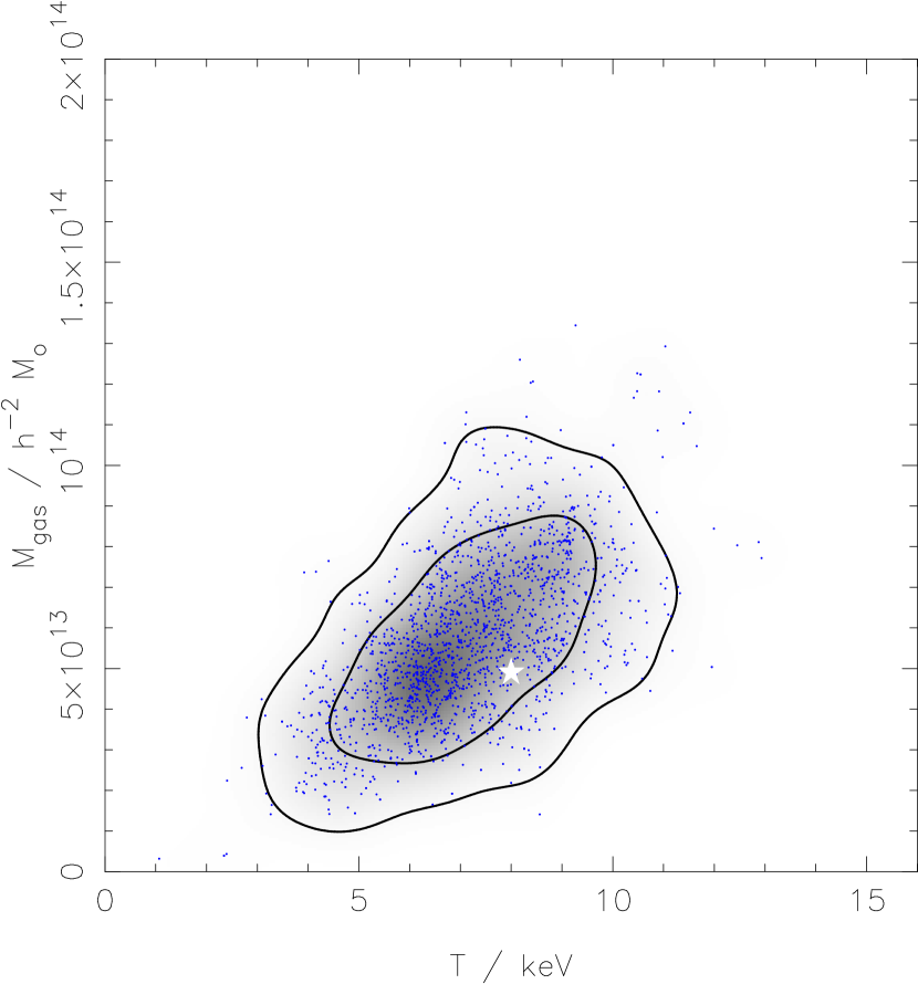
Figure 4: Marginalised probability distributions of cluster astrophysical parameters from mock current experiments. Left: $\textrm{Pr}(M_{200},c|\textrm{\,Data\,},\textrm{\,iHSE\,})$; Right: $\textrm{Pr}(T,M_{\rm gas}|\textrm{\,Data\,},\textrm{\,iHSE\,})$. MCMC samples are shown as points, overlaid on their minimally-smoothed histogram (marked with contours enclosing 68 and 90% of the posterior probability. The white star shows the true parameter values.

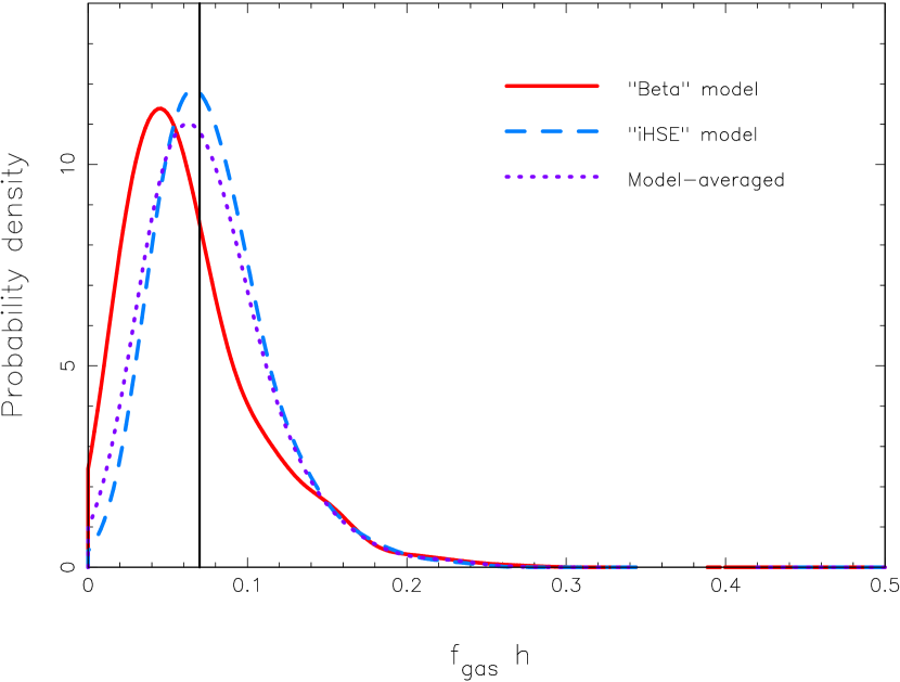
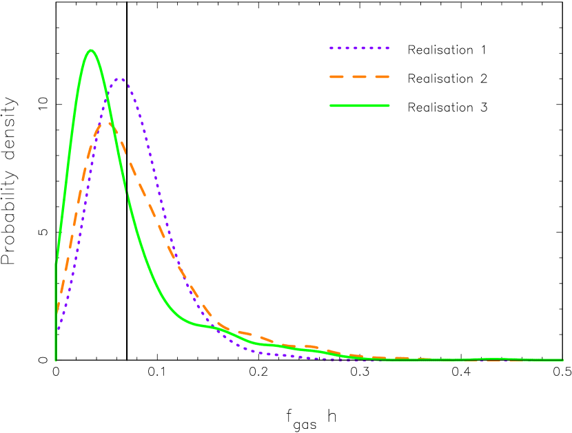
Figure 5: Marginalised probability distributions of cluster cosmological parameters from mock current experiments. Left: Marginalised probability distributions of $f_{\rm gas}h$; the true cluster model is iHSE. $\textrm{Pr}(f_{\rm gas}h|\textrm{\,Data\,},\textrm{\,Beta\,})$ and $\textrm{Pr}(f_{\rm gas}h|\textrm{\,Data\,},\textrm{\,iHSE\,})$ are plotted with full and dashed lines respectively; the dotted curve shows the result of model-averaging, $\textrm{Pr}(f_{\rm gas}h|\textrm{\,Data\,})$. Right: the effect of different CMB realisations on the model-averaged inferences. In both plots the true value of $f_{\rm gas}h$ is shown by the dark solid vertical line.

Example model parameter inferences are shown in Figure 4, where in each panel the posterior density has been marginalised over all but two of the parameter dimensions. The effect of the Gaussian prior on the gas temperature can be seen in the right-hand panel. The estimated precision on each of the three parameters $M_{200}$, $c$, and $M_{\rm gas}$ are 25, 25 and 50 percent respectively.

The left-hand panel of Figure 5 shows the cosmological results from the joint analysis of the current generation low redshift SZ and lensing data. This plot shows the answer to question (iii) as posed in Section 2. The joint evidences calculated for each model, for either given dataset, were equal within the numerical errors; this indicates that the model averaging equation has two terms to be considered, leading to the (quasi) model-independent statement about $f_{\rm gas}$ given in the left panel of the figure.

However, the right-hand panel shows the sensitivity of the VSA SZ data to the contaminant primordial CMB fluctuations: the model-averaged $f_{\rm gas}$ probability distributions show significant variation with CMB realisation. Realisations 1, 2 and 3 correspond to the situations where the cluster lies approximately in front of a primordial CMB saddle point, a shallow trough and a peak respectively. In the latter case the gas mass (and so gas fraction) is then underestimated.

The evidence analysis of CMB realisations 2 and 3 show neither model being preferred by more than a small factor in probability ($<3$) regardless of the true cluster model. In some cases the primordial CMB is being fitted (by the more flexible Beta model) as well as the cluster, and in others the noise is high enough for the Occam factor in the evidence to dominate and the simpler iHSE model is preferred. However, the extent to which the evidence favours either model is never greater than the belief threshold suggested in Section 2. This indicates that the presence of the primordial CMB fluctuations has been dealt with correctly – the inconclusiveness of the evidence ratios ensure that the conclusions drawn about the structure of the cluster are not systematically incorrect.

However the implication of this result is that in order to investigate the astrophysics of low redshift clusters via SZ and gravitational lensing (questions (i) and (ii)), more information is required. This could take the form of multi-frequency SZ observations, to allow better separation of the cluster and primordial CMB components (Lancaster et al. 2003, in preparation), or stronger priors on the cluster parameters. Reducing the freedom of the Beta model to fit the CMB fluctuations will indeed produce more precise gas fraction estimates, but to be confident of the accuracy of these numbers the applied priors should be strongly physically motivated. A good first step in this direction would be to derive joint priors on any model’s parameters from a large sample of hydrodynamically-simulated clusters.

5.3 Next generation experiments

We now move on to consider the kind of observations we can expect from upcoming SZ telescopes such as AMI (Kneissl et al., 2001), the SZA (Mohr et al., 2002) and AMiBA (Lo et al., 2000), in combination with matched lensing observations from wide field optical cameras. Rather than compare the different experiments, we note that they are qualitatively similar instruments and proceed to use AMI, and for the mock lensing observations the ESO Wide Field Imager, as specific examples in this work. AMI will consist of (a) ten close-packed 3.7-m dishes operating at 15GHz and (b) the eight 13-m dishes of the current Ryle Telescope (which are separated by longer baselines). The two parts of this array will have different correlators and therefore provide two independent measurements of the sky, allowing the two datasets to be combined by a simple sum of the individual log-likelihoods.

An important question is that of the strength of the primordial CMB on the angular scales to which AMI is sensitive. These correspond to a maximum $l$-range of 1000 to 6600 for AMI’s small dishes, and 6000 to 36000 for the large Ryle Telescope dishes; note that in practice the minimum $\ell$ values used in observations will be significantly greater. The primordial CMB power spectrum is relatively poorly known in this region, with only the measurements by ACBAR (Runyan et al., 2003) extending to $\ell$ of 2500 and CBI (Pearson et al. 2003; Mason et al. 2003) extending to $\ell$ of 3500. The CBI group find an excess of power at the higher of these wavenumbers, which has been interpreted as being due to the integrated SZ effect of the large-scale structure along the line of sight (Bond et al. 2003). For the purposes of this work we make two assumptions: first, the primordial CMB can be neglected for the Ryle observations at $\ell>6000$, and second that extrapolating the power spectrum of Figure 1 to this $\ell$ limit gives a reasonable estimate of the amplitude of the primordial fluctuations on larger scales. For comparison with the latter we also simulated short baseline data with no contribution to the noise from the CMB.

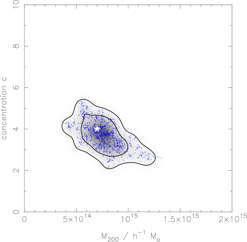
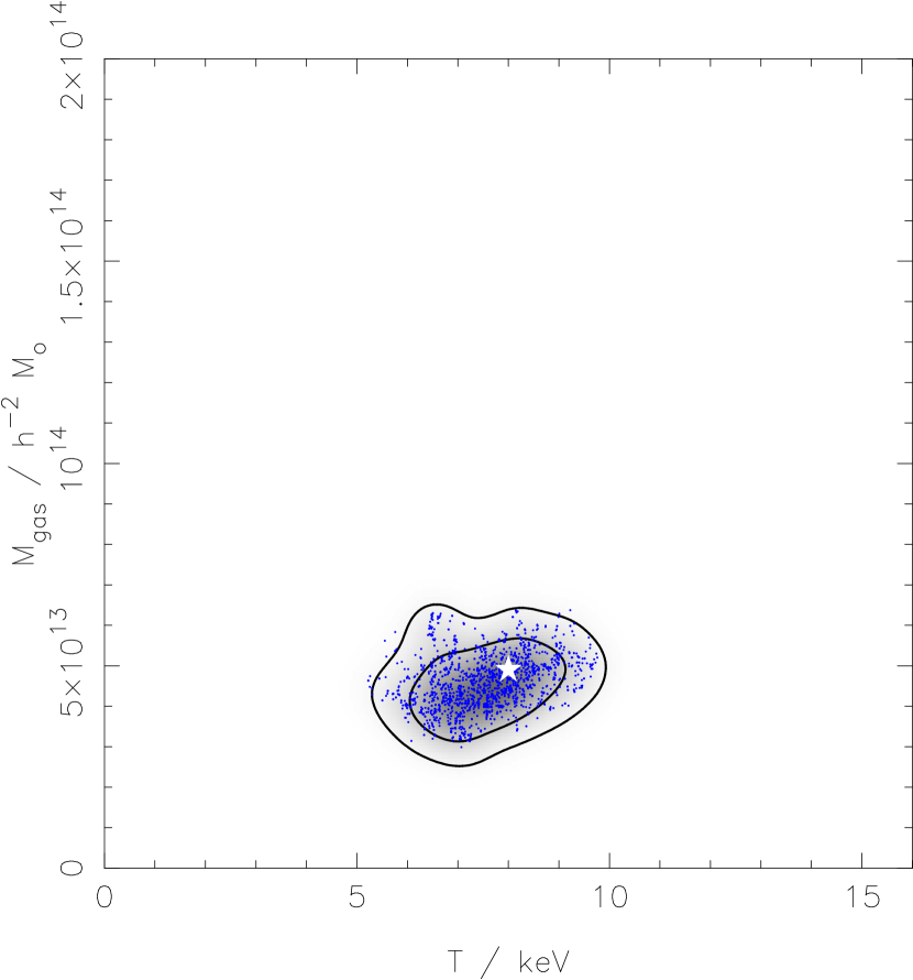
Figure 6: Marginalised probability distributions of cluster astrophysical parameters from mock next-generation experiments. Left: $\textrm{Pr}(M_{200},c|\textrm{\,Data\,},\textrm{\,iHSE\,})$; Right: $\textrm{Pr}(T,M_{\rm gas}|\textrm{\,Data\,},\textrm{\,iHSE\,})$. MCMC samples are shown as points, overlaid on their minimally-smoothed histogram (marked with contours enclosing 68 and 90% of the posterior probability. The white star shows the true parameter values.

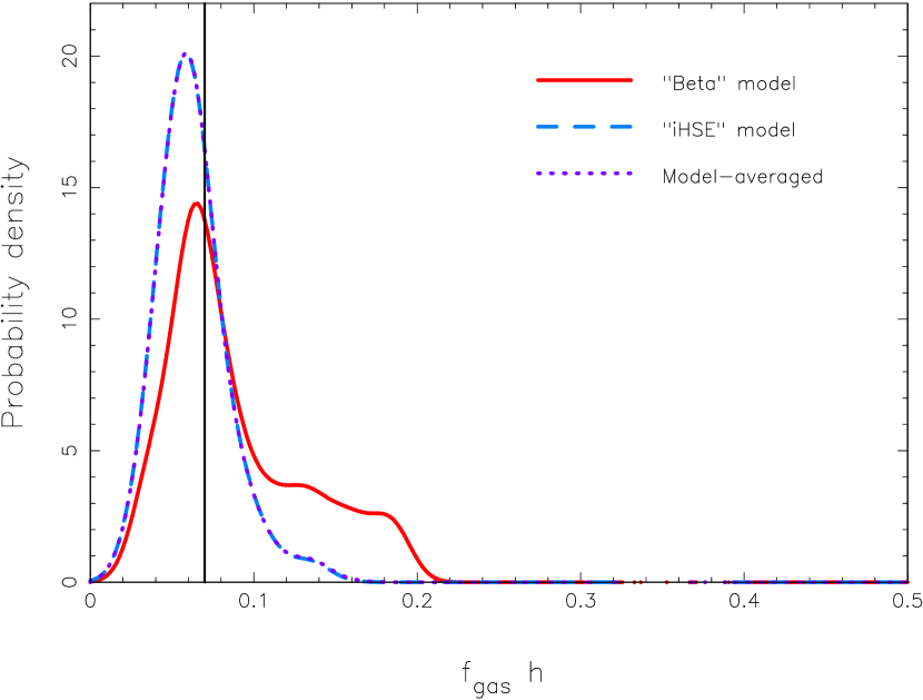
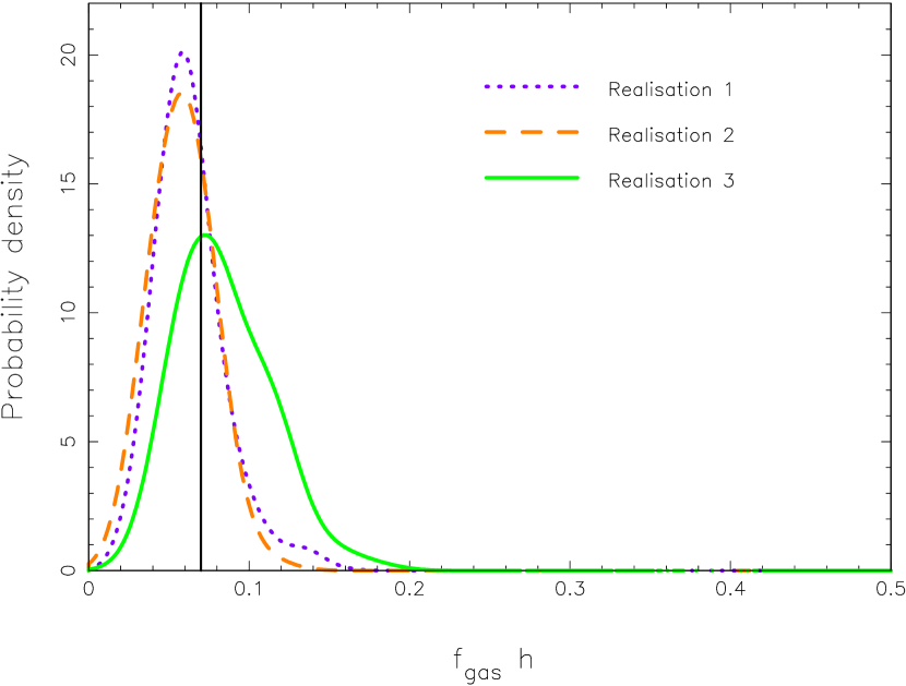
Figure 7: Marginalised probability distributions of cluster cosmological parameters from mock next-generation experiments. Left: Marginalised probability distributions of $f_{\rm gas}h$; the true cluster model is iHSE. $\textrm{Pr}(f_{\rm gas}h|\textrm{\,Data\,},\textrm{\,Beta\,})$ and $\textrm{Pr}(f_{\rm gas}h|\textrm{\,Data\,},\textrm{\,iHSE\,})$ are plotted with solid and dashed lines respectively; the dotted curve shows the result of model-averaging, $\textrm{Pr}(f_{\rm gas}h|\textrm{\,Data\,})$, and is indistinguishable from the (correctly) selected model curve. Right: the effect of different CMB realisations on the model-averaged inferences. In both plots the true value of $f_{\rm gas}h$ is shown by the dark solid vertical line.

Example model parameter inferences from this quality data are shown in Figure 6, where in each panel the posterior density has been marginalised over all but two of the parameter dimensions. The effect of the Gaussian prior on the gas temperature can be seen in the right-hand panel. The estimated model-dependent precisions on each of the three parameters $M_{200},c$ and $M_{\rm gas}$ are 20, 20, and 12 percent respectively. The improvement in the results from the lensing data is slight, the increased lensing strength being balanced by the decreased number of observed background galaxies due to the smaller field of view. The improvement in gas mass estimation is more marked, due to a combination of reduced primordial CMB at the higher $l$-values, and the more comprehensive $uv$-plane coverage afforded by AMI.

Table 2: Evidence ratios from the joint analysis of the “next-generation” mock observations; this quantity is given by $\textrm{Pr}(\textrm{\,Data\,}|\textrm{correct model})/\textrm{Pr}(\textrm{\,Data\,}|\textrm{incorrect model})$ and so should be greater than unity if accurate astrophysical conclusions are to be drawn.

CMB included?	Model	Evidence ratio (CMB realn. 1, 2, 3)
Yes	Beta	1.5, 81, 2.5
	iHSE	110, 110, 37
No	Beta	20
	iHSE	600

Table 2 gives the evidence ratios for the experiments outline above. In the case where no contaminant primordial CMB is present the most probable model matches that used in simulating the data. The factor by which the true model is more likely is larger when the iHSE model is used: this model is both simpler, and it provides a better fit. The same is true when the primordial fluctuations are present, with suitably (but not greatly) reduced evidence ratios, with the variation in the evidence ratios being due to differing noise realisations. We again see the sensitivity to the noise realisation, with confident model selection possible in only 4 out of the 6 analyses. For the Beta model cluster, the same balance between model complexity and goodness of fit is seen as in Section 5.2, suggesting the need for informative priors even for this higher quality data.

Figure 7 shows the cosmological inference drawn from the analysis of the mock iHSE cluster. The model-averaged $f_{\rm gas}h$ probability distributions are dominated by the iHSE model contribution – this astrophysical model has been successfully selected by the evidence. Taking the median sample as an estimator for the gas fraction we find $f_{\rm gas}h=(0.061^{+0.019}_{-0.015})$. With no CMB contamination this estimate changes to $f_{\rm gas}h=(0.054^{+0.015}_{-0.013})$, an increase in precision of just 5% (from 28 to 23%). This is an indication of the small contribution to the error budget that the primordial CMB has at these angular scales. Indeed, as previously mentioned the shortest AMI baseline will be longer than that used in this work, such that the effect of the primordial CMB will be reduced; we might therefore expect results lying inbetween the two situations simulated here.

6 Discussion

The analysis of the simulated data presented in the previous section was designed to be a simple demonstration of a general methodology. In the current section we discuss the advantages and disadvantages of our approach, and its ability to be extended, beginning with some comparison with other methods currently in use.

The Bayesian method described here can be seen as a generalisation of the model fitting procedures employed by other workers. For example, King et al. (2002) fitted lens models with 1, 2 and 3 parameters to weak shear data for Abell 1689 by the maximum likelihood method; they compute likelihood contours for the parameter uncertainties and compare the models’ goodness of fit with the likelihood ratio test. As explained in Section 2, such a grid-based computation is not practical with the 6–8 parameters used here. Indeed, numerical maximisation of a function of 6–8 variables is already a demanding problem, especially when there are multiple maxima to be investigated. Comparing models by their maximum likelihoods is also rather sensitive to noise features in the data, rather than assessing the relative appropriateness of the models to the task of explaining the data. The maximum likelihood ratio is formally equivalent to the evidence ratio when the prior pdf is a delta-function at the best-fit point: this is clearly not an accurate representation of our prior knowledge. The $\chi^{2}$ fitting of SZ visibility data by Grego et al. (2001), and the joint maximum likelihood analysis of SZ and X-ray data of Reese et al. (2002) are two other examples of a small number of parameters being fitted within the context of a single cluster model; one of the aims of this work was to provide a complete framework which combined and extended analyses such as these.

Other methods proposed for use in the joint analysis of cluster data have, to date, been focused on “parameter–free” reconstruction. Reblinsky (2000) suggests an iterative procedure for refining the cluster potential using X-ray, SZ and weak lensing images, whilst Zaroubi et al. (2001) provide a direct inversion method to take these images and produce a three-dimensional cluster model, making use of some attractive features of working in the Fourier domain. Doré et al. (2001) suggest using SZ and weak lensing data to constrain successive orders of perturbation from spherical symmetry, again working from ready-made maps. All these methods have been shown to work well with noiseless input. However, those working with the observations have opted to increase the complexity of their cluster models in a more gradual way, for example fitting an X-ray map with a simple model and using this model to predict the observed SZ effect (e.g. Jones et al., 2001). The method described here is this common sense reduced to calculation – the use of simple functions for the potential, gas density and temperature allows the model complexity to be tuned to the data quality via the evidence. The “parameter-free” methods referred to above actually have many parameters, usually the values of pixels in a grid: direct methods will produce one set of parameters, but these may not be the most probable given the data, or even the most appropriate given the parameter degeneracies. When trying to measure quantities such as the gas fraction, all the cluster configurations allowed by the data should be accounted for, in order to calculate an accurate confidence interval; only by fully exploring a model’s parameter space this can be achieved. Indeed, consideration of a range of models is then desirable to gain the next level of accuracy, one that is model-independent in the sense of the discussion in Section 2. Sampling from a model’s parameter space produces the set of cluster configurations permitted by the data, which is arguably more useful than the unique solutions generated by direct methods.

One might wonder how the MCMC technique endorsed in this work would perform if used in the many-parameter modelling of the type mentioned above. Indeed, in this context the number of parameters included here is rather small. The evidence itself is a guide in the development of these methods, providing a handle on the information content of the data: if the evidence does not favour a triaxial ellipsoid over a spherical model, then it might reasonably be assumed not to favour a “parameter-free” representation. The ability of a sampler to cope with increasing numbers of parameters is somewhat sensitive to the shape of the posterior distribution under investigation; we find that including extra nuisance parameters (the parameters of point sources contaminating the SZ data for example) does not affect the accuracy of the posterior exploration (Lancaster et al. 2003 in preparation), and neither does increasing the number of sub-clumps when modelling gravitational lenses with multiple mass concentrations (Kneib et al., 2003). Moving to three-dimensional cluster modelling introduces a number of strong degeneracies in the parameter space (Fox & Pen, 2002) which may well require a tailor-made MCMC sampler instead of the general purpose engine used here. Such a sampler might be expected to reduce the run-time of the method, which (compared to a direct inversion or a downhill simplex $\chi^{2}$ minimisation) is its major disadvantage: to produce each posterior distribution shown in the figures of this paper a computation time of several hours with a 1 GHz processor was required. The evidence calculation takes rather longer, since the numerical precision comes from repeated posterior explorations. The computation time scales approximately as $N_{\rm data}\times N_{\rm parameters}$ (Gilks et al., 1996), prompting careful design of the sampler and likelihood calculation. However, the alternatives for coping with noisy data can be just as time consuming; for instance resampling of the data to generate confidence limits (e.g. Allen et al., 2003) effectively performs the same calculations as the MCMC process, but with more limited output. Nevertheless, it is the computational cost of the method that is perhaps the most urgent aspect to be addressed in further work.

7 Conclusions

We have developed an algorithm based on the Markov-Chain Monte-Carlo technique for investigating simple but many-parameter models of clusters. The method allows straightforward inclusion of many datasets, correctly weighting each datapoint according to its assumed likelihood; by exploring the posterior probability distribution rather than the likelihood we can incorporate information on the cluster from other sources via the parameter prior densities. Calculation of the Bayesian evidence by thermodynamic integration during the burn-in period can be done to sufficient accuracy to allow different astrophysical models to be compared; this statistic automatically includes the common-sense of Occam’s razor, allowing movement away from the simplest assumed models only when the data require it.

Applying the method to simulated weak gravitational lensing and interferometric Sunyaev-Zel’dovich effect data we draw the following conclusions:

• Gravitational weak lensing data allow cluster mass distribution model parameters to be estimated with a precision of around 20 percent over the small range of low redshifts discussed here.

• Primordial CMB anisotropies contaminate SZ observations on angular scales less than $l\approx 1000$. However, the nature of the primordial fluctuations allows them to be properly accounted for in the likelihood function, preventing inaccurate conclusions about either the cluster model or the gas fraction. The available precision on the cluster gas mass increases by a factor of approximately two (to around 10 percent) when moving from instruments such as the VSA to those more like AMI.

• The behaviour of the Bayesian evidence as a model selection tool can be understood in terms of both goodness of fit and model complexity; in the case of the primordial CMB contaminated data, the more flexible fitting formulae are sometimes favoured by the evidence as they provide a better fit to all the data, prompting the need for improved prior constraints on the model parameters. One recommended source of these priors is a sample of numerically simulated clusters.

• Where the SZ data are less contaminated by the primordial CMB the evidence does indeed allow successful astrophysical model selection, leading to accurate conclusions about the dynamical state of the cluster under observation.

• Where the evidences for a range of models are of comparable size, a correctly weighted average may be taken, resulting in appropriately precise inferred uncertainties on the parameter in question – for the gas fraction $f_{\rm gas}h$ we may expect a model-independent uncertainty on this parameter of around 50 percent for a low redshift cluster, and under 30 percent with observations of a cluster with AMI.

This last point is one worth returning to; under the assumption of a Universal cluster gas fraction the model-independent inference for each independent member of a sample of $N$ clusters can be combined by straightforward multiplication of their posterior probability distributions, reducing the uncertainty on this parameter by a factor of approximately $\sqrt{N}$.

The work described in this paper is straightforwardly extendable to incorporate X-ray, and indeed any other, cluster data. Similarly, investigating more complex cluster models by relaxing the assumptions of isothermality, spherical symmetry and a single cluster potential is easy to do, with the evidence providing the self-consistent and logical way through the astrophysical model analysis. The obvious immediate next step to take is the inclusion of the X-ray data, and the opening up of another dimension of cosmological parameter space, that of the Hubble parameter: this analysis applied to clusters observed with the VSA will be the subject of future publications.

Acknowledgments

We thank Sarah Bridle, Keith Grainge, Steve Gull, Katy Lancaster, Charles McLachlan and Richard Saunders for helpful discussions, and are very grateful to John Skilling of MaxEnt Data Consultants for making his MCMC software BayeSys3 available to us. We thank the anonymous referee for suggestions that improved the readability of the article. PJM acknowledges the PPARC, and AS acknowledges St. John’s College, Cambridge, for financial support in the form of research studentships.

References

- Allen et al. (2002) Allen S., Schmidt R., A.C. F., 2002, MNRAS, 334, L11
- Allen et al. (2003) Allen S. W., Schmidt R. W., Fabian A. C., Ebeling H., 2003, MNRAS, 342, 287
- Battye & Weller (2003) Battye R. A., Weller J., 2003, ArXiv Astrophysics e-prints, p. 5568
- Birkinshaw & Hughes (1994) Birkinshaw M., Hughes J. P., 1994, ApJ, 420, 33
- Bond & The CBI Collaboration (2003) Bond J., The CBI Collaboration 2003, ArXiv Astrophysics e-prints, p. 5386
- Bridle et al. (2001) Bridle S., Gull S., Bardeau S., Kneib J.-P., 2001, in Natarajan P., ed., The Shapes of Galaxies and their Dark Halos Proc. of the Yale Cosmology Workshop, A new method for determining galaxy shapes. World Scientific
- Carlstrom et al. (1996) Carlstrom J. E., Joy M., Grego L., 1996, ApJL, 456, L75
- Castander et al. (2000) Castander F. J., Holder G. P., Clowe D., Carlstrom J. E., Schirmer M., Reese E., Kneib J.-P., 2000, in Constructing the Universe with Clusters of Galaxies Combining SZ, X-rays and Lensing Data on the Cluster of Galaxies CL0016
- Cavaliere et al. (1978) Cavaliere A., Danese L., de Zotti G., eds, 1978, Hubble constant from X-ray and microwave observations of clusters of galaxies
- Clowe & Schneider (2002) Clowe D., Schneider P., 2002, A&A, 395, 385
- Dahle et al. (2002) Dahle H. ., Kaiser N., Irgens R. J., Lilje P. B., Maddox S. J., 2002, ApJS, 139, 313
- Doré et al. (2001) Doré O., Bouchet F. R., Mellier Y., Teyssier R., 2001, A&A, 375, 14
- Evrard et al. (2002) Evrard A. E., MacFarland T. J., Couchman H. M. P., Colberg J. M., Yoshida N., White S. D. M., Jenkins A., Frenk C. S., Pearce F. R., Peacock J. A., Thomas P. A., 2002, ApJ, 573, 7
- Fox & Pen (2002) Fox D. C., Pen U., 2002, ApJ, 574, 38
- Gilks et al. (1996) Gilks W. R., Richardson S., Spiegelhalter D. J., 1996, Markov-Chain Monte-Carlo In Practice. Cambridge: Chapman and Hall
- Grainge et al. (2002) Grainge K., Jones M. E., Pooley G., Saunders R., Edge A., Grainger W. F., Kneissl R. ., 2002, MNRAS, 333, 318
- Grainger et al. (2002) Grainger W. F., Das R., Grainge K., Jones M. E., Kneissl R., Pooley G. G., Saunders R. D. E., 2002, MNRAS, 337, 1207
- Grego et al. (2001) Grego L., Carlstrom J. E., Reese E. D., Holder G. P., Holzapfel W. L., Joy M. K., Mohr J. J., Patel S., 2001, ApJ, 552, 2
- Hobson et al. (2002) Hobson M. P., Bridle S. L., Lahav O., 2002, MNRAS, 335, 377
- Hobson & Maisinger (2002) Hobson M. P., Maisinger K., 2002, MNRAS, 334, 569
- Hoekstra et al. (2000) Hoekstra H., Franx M., Kuijken K., 2000, ApJ, 532, 88
- Jaynes (2003) Jaynes E., 2003, Probability Theory: The Logic of Science. Cambridge: CUP
- Jeffreys (1932) Jeffreys H., 1932, Proc. Roy. Soc., 138, 48
- Jenkins et al. (2001) Jenkins A., Frenk C. S., White S. D. M., Colberg J. M., Cole S., Evrard A. E., Couchman H. M. P., Yoshida N., 2001, MNRAS, 321, 372
- Jones et al. (2001) Jones M., Edge A., Grainge K., Grainger W., Kneissl R., Pooley G., Saunders R., Miyoshi S., Tsuruta T., Yamashita K., Tawara Y., Furuzawa A., Harada A., I. H., 2001, H0 from an orientation-unbiased sample of SZ and X-ray clusters, submitted to MNRAS
- Jones et al. (1993) Jones M. E., Saunders R., Alexander P., Birkinshaw M., Dillon N., Grainge K., Hancock S., Lasenby A., Lefebvre D., Pooley G., 1993, Nature, 365, 320
- Joy et al. (2001) Joy M., LaRoque S., Grego L., Carlstrom J. E., Dawson K., Ebeling H., Holzapfel W. L., Nagai D., Reese E. D., 2001, ApJL, 551, L1
- Kaiser & Squires (1993) Kaiser N., Squires G., 1993, ApJ, 404, 441
- Kaiser et al. (1995) Kaiser N., Squires G., Broadhurst T., 1995, ApJ, 449, 460
- King et al. (2002) King L. J., Clowe D. I., Schneider P., 2002, A&A, 383, 118
- Kneib et al. (2003) Kneib J., Hudelot P., Ellis R. S., Treu T., Smith G. P., Marshall P., Czoske O., Smail I., Natarajan P., 2003, ArXiv Astrophysics e-prints
- Kneissl et al. (2001) Kneissl R., Jones M. E., Saunders R., Eke V. R., Lasenby A. N., Grainge K., Cotter G., 2001, MNRAS, 328, 783
- Lahav et al. (2000) Lahav O., Bridle S. L., Hobson M. P., Lasenby A. N., Sodré L., 2000, MNRAS, 315, L45
- LaRoque et al. (2003) LaRoque S. J., Joy M., Carlstrom J. E., Ebeling H., Bonamente M., Dawson K. S., Edge A., Holzapfel W. L., Miller A. D., Nagai D., Patel S. K., Reese E. D., 2003, ApJ, 583, 559
- Lay & Halverson (2000) Lay O. P., Halverson N. W., 2000, ApJ, 543, 787
- Lo et al. (2000) Lo K. Y., Chiueh T., Liang H., Ma C. P., Martin R., Ng K.-W., Pen U. L., Subramanyan R., 2000, in IAU Symposium AMiBA: an Array for Microwave Background Anisotropy
- MacKay (1992) MacKay D., 1992, Neural Computation, 4, 415
- Marshall et al. (2002) Marshall P. J., Hobson M. P., Gull S. F., Bridle S. L., 2002, MNRAS, 335, 1037
- Mason & and the CBI Collaboration (2003) Mason B. S., and the CBI Collaboration 2003, ArXiv Astrophysics e-prints, p. 5384
- Mason et al. (2001) Mason B. S., Myers S. T., Readhead A. C. S., 2001, ApJL, 555, L11
- Mohr et al. (2002) Mohr J. J., Carlstrom J. E., The SZA Collaboration 2002, in ASP Conf. Ser. 257: AMiBA 2001: High-Z Clusters, Missing Baryons, and CMB Polarization The SZ-Array: Configuration and Science Prospects. p. 43
- Navarro et al. (1995) Navarro J., Frenk C., White S., 1995, MNRAS, 275, 720
- Pearson & and the CBI Collaboration (2003) Pearson T., and the CBI Collaboration 2003, ArXiv Astrophysics e-prints, p. 5388
- Press & Schechter (1974) Press W., Schechter P., 1974, ApJ, 187, 425
- Reblinsky (2000) Reblinsky K., 2000, A&A, 364, 377
- Reese et al. (2002) Reese E. D., Carlstrom J. E., Joy M., Mohr J. J., Grego L., Holzapfel W. L., 2002, ApJ, 581, 53
- Runyan et al. (2003) Runyan M. C., Ade P. A. R., Bock J. J., Bond J. R., Cantalupo C., Contaldi C. R., Daub M. D., Goldstein J. H., Gomez P. L., Holzapfel W. L., Kuo C. L., Lange A. E., Lueker M., Newcomb M., Peterson J. B., Pogosyan D., Romer A. K., Ruhl J., Torbet E., Woolsey D., 2003, ArXiv Astrophysics e-prints, p. 5553
- Sarazin (1988) Sarazin C., 1988, X-ray Emission from Clusters of Galaxies. Cambridge: CUP
- Schneider et al. (2000) Schneider P., King L., Erben T., 2000, A&A, 353, 41
- Schramm & Kayser (1995) Schramm T., Kayser R., 1995, A&A, 289, L5
- Seitz et al. (1998) Seitz S., Schneider P., Bartelmann M., 1998, A&A, 337, 325
- Sheth et al. (2001) Sheth R. K., Mo H. J., Tormen G., 2001, MNRAS, 323, 1
- Slosar & and the VSA Collaboration (2003) Slosar A., and the VSA Collaboration 2003, MNRAS, 341, L29
- Sunyaev & Zeldovich (1972) Sunyaev R. A., Zeldovich Y. B., 1972, Comments on Astrophysics, 4, 173
- Suto et al. (1998) Suto Y., Sasaki S., Makino N., 1998, ApJ, 509, 544
- Taylor & and the VSA Collaboration (2003) Taylor A., and the VSA Collaboration 2003, MNRAS, 341, 1066
- Watson & and the VSA Collaboration (2003) Watson R. A., and the VSA Collaboration 2003, MNRAS, 341, 1057
- White et al. (1993) White S., Navarro J., Evrard A., Frenk C., 1993, Nature, 366, 429
- Wright & Brainerd (2000) Wright C. O., Brainerd T. G., 2000, ApJ, 534, 34
- Zaroubi et al. (2001) Zaroubi S., Squires G., de Gasperis G., Evrard A. E., Hoffman Y., Silk J., 2001, ApJ, 561, 600