Modelling Collision Products of Triple-Star Mergers

Abstract

In dense stellar clusters, binary-single and binary-binary encounters can ultimately lead to collisions involving two or more stars during a resonant interaction. A comprehensive survey of multi-star collisions would need to explore an enormous amount of parameter space, but here we focus on a number of representative cases involving low-mass (0.4, 0.6, and $0.8{\rm M}_{\odot}$) main-sequence stars. Using both Smoothed Particle Hydrodynamics (SPH) calculations and a much faster fluid sorting software package (MMAS), we study scenarios in which a newly formed product from an initial collision collides with a third parent star. By varying the order in which the parent stars collide, as well as the orbital parameters of the collision trajectories, we investigate how factors such as shock heating affect the chemical composition and structure profiles of the collision product. Our simulations and models indicate that the distribution of most chemical elements within the final product is not significantly affected by the order in which the stars collide, the direction of approach of the third parent star, or the periastron separations of the collisions. Although the exact surface abundances of beryllium and lithium in the product do depend on the details of the dynamics, these elements are always severely depleted due to mass loss during the collisions. We find that the sizes of the products, and hence their collisional cross sections for subsequent encounters, can be sensitive to the order and geometry of the collisions. For the cases that we consider, the radius of the product formed in the first (single-single star) collision ranges anywhere from roughly 2 to 30 times the sum of the radii of its parent stars. The size of the final product formed in our triple-star collisions is more difficult to determine, but it can easily be as large or larger than a typical red giant. Although the vast majority of the volume in such a product contains diffuse gas that could be readily stripped in subsequent interactions, we nevertheless expect the collisional cross section of a newly formed product to be greatly enhanced over that of a thermally relaxed star of the same mass. Our results also help establish that the algorithms of MMAS can quickly reproduce the important features of our SPH models for these collisions, even when one of the parent stars is itself a former product.

1 Introduction

1.1 Motivations

One exciting aspect of dense stellar systems is the simultaneous importance of three principal areas of stellar astrophysics: dynamics, evolution, and hydrodynamics. Many simulation codes focus on one of these areas and have often been lifelong works in progress. The first attempts at unifying these treatments into a coherent model to describe clusters have begun only recently. In June 2002, specialists in stellar dynamics, stellar evolution, hydrodynamics, cluster observation, visualization, and computer science gathered at the American Museum of Natural History in New York City to begin discussing a framework for MOdelling DEnse STellar systems, without having to MODify Existing STellar codes extensively. The workshop-style meeting, organized by P. Hut and M. Shara, became known as MODEST-1 (Hut et al., 2003). The second such meeting, MODEST-2, was organized by S. Portegies Zwart and P. Hut and held in December 2002 at the Anton Pannekoek Institute in Amsterdam (Sills et al., 2003). From MODEST-2, a set of eight “working groups” were established, each focusing on a different aspect of the MODEST endeavour. Attempting to integrate stellar dynamics, evolution, and hydrodynamics codes into one fully functional package will be challenging, largely because each area treats stellar properties that evolve on different time-scales. However, by combining these areas, we will be able to better model the origins, dynamics, evolution, and death of globular clusters, galactic nuclei, and other dense stellar systems.

In this paper, our focus is on modelling hydrodynamic interactions between stars. The goal is to develop a software module for quickly generating collision product models, ultimately for any type of stellar collision, that could be incorporated into simulations of dense star clusters. Lombardi et al. (2002) presented an appropriate formulation for treating parabolic single-single star collisions between low-mass main-sequence stars. Here we extend that study to include situations in which one of the parent stars is itself a thermally unrelaxed collision product. Such scenarios can occur during binary-single or binary-binary interactions, when the time between collisions is much less than the thermal relaxation time-scale.

Stellar collisions and mergers can strongly affect the overall energy budget of a cluster and even alter the timing of important dynamical phases such as core collapse. Furthermore, hydrodynamic interactions are believed to produce a number of non-canonical objects, including blue stragglers, low-mass X-ray binaries, recycled pulsars, double neutron star systems, cataclysmic variables, and contact binaries. Such stars and systems are among the most challenging to model, but they are also among the most interesting observational markers. Blue stragglers, for example, exist on an extension of the main-sequence, but beyond the turnoff point. Blue stragglers are therefore appropriately named, as they are more blue than the remaining ordinary main-sequence stars, and, compared to other stars of similar mass, are straggling behind in their evolution. This aberration from the common path of stellar evolution is believed to be due to mass transfer or merger in a binary system, or from the direct collision of two or more main-sequence stars (for a review, see Bailyn, 1995). Predicting the numbers, distributions, and other observable characteristics of stellar exotica will be essential for detailed comparisons with observations.

1.2 Stellar dynamics and stellar evolution

Stellar dynamics codes determine the motions of stars. The primary approaches to evolving clusters or galactic nuclei dynamically are direct N-body integrations (e.g., Portegies et al., 1997; Hurley et al., 2001), solving the Fokker-Planck equation (e.g., Takahashi & Portegies Zwart, 2000), Monte Carlo approaches (e.g., Watters et al., 2000; Joshi, Rasio, & Portegies Zwart, 2000; Joshi, Nave, & Rasio, 2001; Freitag & Benz, 2002; Giersz, 2001; Giersz & Spurzem, 2003), and gaseous models (e.g., Spurzem & Takahashi, 1995). For a review of the ongoing NBODY effort for accurate N-body simulations, see Aarseth (1999); for a general review of cluster dynamics, see Meylan & Heggie (1997) and Heggie & Hut (2003).

The most important quantities that a stellar evolution software module can provide to a dynamics module are the stellar masses, as well as the stellar radii if collisions are included. At least in principle, these results could come from a live (i.e., concurrent with the cluster dynamics) stellar evolution calculation, from fitting formulae, or from interpolation among prior calculations. Due to the large number of stars, it would be wasteful to expend a considerable amount of time for a live computation of each star’s evolution. For the ordinary stars whose evolution is not perturbed by an event such as a collision, it is much more efficient and entirely appropriate to interpolate among, or to use analytic fitting formulae based upon, previously calculated evolutionary tracks. The parameter space associated with non-canonical stars, however, is too enormous to be adequately covered by interpolation or fitting formulae, and it will ultimately be necessary to invoke a full stellar evolution calculation in parallel with the stellar dynamics for such stars. Although live stellar evolution calculations have not yet been combined with stellar dynamics codes, some parametrized codes, such as SeBa (Portegies Zwart & Verbunt, 1996), SSE (Hurley, Pols, & Tout, 2000) and BSE (Hurley, Tout, & Pols, 2002), have been successfully integrated (Portegies et al., 1997; Portegies Zwart et al., 2001; Shara & Hurley, 2002).

When physical collisions between stars are modelled in a cluster calculation or a scattering experiment, it is usually done using a method known as “sticky particles,” in which a collision product is given a mass equal to the combined mass of the two parent stars and a velocity determined by momentum conservation. In a collision between two main-sequence stars, for example, the result would be modelled as a rejuvenated, thermally relaxed main-sequence star. This simple method is a reasonable first approximation for many situations. However, there are important characteristics of collision products that are neglected, including their rapid rotation, peculiar composition profiles, and enhanced sizes due to shock heating. If the thermal relaxation time-scale of the collision product is much less than the time until its next collision, then it is appropriate to assume the product becomes instantaneously thermally relaxed, as is done in the classic simulations of Quinlan & Shapiro (1990). This approximation becomes questionable when the collision has been mediated by a binary, as there is then at least one star in the immediate vicinity of the collision product and the likelihood of a subsequent collision will depend sensitively on the product’s thermally unrelaxed size.

Binaries are subject to enhanced collision rates for two primary reasons: (1) their collision cross section depends on the semi-major axis of the orbit, as opposed to the radius of a single star, and (2) due to mass segregation, binaries tend to be found in the core of the cluster, the densest and most active region. In clusters with a binary fraction exceeding about 20 per cent, binary-binary collisions are expected to occur more frequently than single-single and binary-single collisions combined (Bacon, Sigurdsson, & Davies, 1996). It is probably not uncommon for binary fractions to be this large: the inner core of NGC 6752, for example, is thought to have a binary fraction in the range 15–38 per cent (Rubenstein & Bailyn, 1997).

Binary populations can lead to complex and chaotic resonant interactions. These interactions tend to exchange energy between the binaries and the other stars in the cluster, and therefore are critical in determining its dynamics and observable characteristics (Hut et al., 1992; Vesperini & Chernoff, 1994). A star intruding on a binary could, depending on parameters such as the separation of the binary and the velocity of the incoming star, escape to infinity, destroy the binary, form a new binary with a star from the original, or form a triple. The outcomes of three body encounters can be categorized using a nomenclature based upon typical atomic processes (see Heggie, 1975, who introduced the use of terms like “ionization” and “exchange,” to describe resultant scenarios). See Hurley & Shara (2002) for an informative narration of the intimate interactions, usually involving binaries, that stars regularly undergo during cluster evolution.

The STARLAB computing environment is a very useful tool for modelling and analyzing all types of stellar phenomena. The general technique for using STARLAB to determine the cross sections or branching ratios for the various outcomes of binary interactions is presented by McMillan & Hut (1996). They also highlight an example set of cases in which a $0.6{\rm M}_{\odot}$ star intrudes upon a binary with a $0.8{\rm M}_{\odot}$ primary and a $0.4{\rm M}_{\odot}$ secondary. Their assumed mass radius relation, $M/{\rm M}_{\odot}=R/{\rm R}_{\odot}$, is appropriate for thermally relaxed main sequence stars and is applied both to the parent stars and any collision products. They find that for binaries with semimajor axes of 0.2, 0.1, 0.05, and 0.02 AU, triple-star mergers comprise about 1, 2, 5, and 15 per cent, respectively, of all merger events. As the results of the present paper will help show, we expect that accounting for the enhanced, thermally unrelaxed size of the first collision product will greatly increase these percentages as well as the range of semimajor axes in which triple-star mergers are significant.

Simulations of moderately dense galactic nuclei initially containing solar-mass main-sequence stars demonstrate that runaway mergers can readily produce stars with masses $\ga 100{\rm M}_{\odot}$. These massive stars then undergo further mergers to produce seed black holes with masses as large as $\sim 10^{3}{\rm M}_{\odot}$ (Quinlan & Shapiro, 1990). This process may be responsible for massive black holes at the centres of most galaxies, including our own. For star clusters, recent N-body simulations reveal that runaway mergers can lead to the creation of central black holes within a few million years (e.g., Portegies Zwart et al., 1999; Portegies Zwart & McMillan, 2002). With the help of Monte Carlo simulations, Rasio, Freitag, & Gürkan (2003) show that the runaway process will occur in a typical cluster with a relaxation timescale less than about 30 Myr. Observational evidence for a possible intermediate-mass black hole in M15 has been recently reported by Gerssen et al. (2002), although the data is more reasonably modelled with a large concentration of stellar-mass compact objects (Baumgardt et al., 2003; Gerssen et al., 2003).

1.3 Stellar hydrodynamics

Mass loss and expansion due to shock heating when two stars collide are examples of hydrodynamical processes that can ultimately affect the future evolution of the cluster. Mostly using the Smoothed Particle Hydrodynamics (SPH, see §2.1) method, numerous scenarios of stellar collisions and mergers have been simulated in recent years, including collisions between two main-sequence stars (Benz & Hills, 1987; Lai, Rasio & Shapiro, 1993; Lombardi et al., 1996; Ouellette & Pritchet, 1998; Sandquist et al., 1997; Sills & Lombardi, 1997; Sills et al., 1997, 2001, 2002; Freitag & Benz, 2003), collisions between a giant star and compact object (Rasio & Shapiro, 1991), and common envelope systems (Rasio & Livio, 1996; Terman et al., 1994, 1995; Sandquist et al., 1998, 2000). The first published SPH calculations of three-body encounters were done by Cleary & Monaghan (1990), who performed over 100 very low resolution simulations and implemented a mass-radius relation appropriate for white dwarfs. Other three- and four-body interaction simulations include binary-binary encounters among $n=1.5$ polytropes (Goodman & Hernquist, 1991) as well as neutron star – main-sequence binary encounters with a neutron star, main-sequence or white dwarf intruder (Davies, Benz & Hills, 1994). See Rasio & Lombardi (1999) for more information concerning the use of SPH in stellar collisions, and see Shara (2002) for a qualitative overview of the progress in stellar collision research.

If the structure and composition profiles of colliding stars were available (perhaps from a live stellar evolution calculation) during a cluster simulation, then the sticky particle method could be replaced by a more detailed hydrodynamics module. SPH calculations could then, at least in principle, be run on demand within this cluster simulation in order to determine the orbital trajectory of the product(s), as well as their structure and chemical composition distributions. However, at least $10^{5}$ SPH fluid particles may be necessary to allow an accurate treatment of the subsequent evolution of collision products (Sills et al., 2002). The trouble, therefore, is that the integration of just a single interaction could consume hours, days or even weeks of computing time (depending on the initial conditions, desired resolution, and available computational resources). Although the use of equal-mass particles, or the more accurate SPH equations of motion derived by Springel & Hernquist (2002), or both, could decrease the total number of particles required, it is still currently impractical to implement a full hydrodynamics calculation for every close stellar encounter during a cluster simulation.

One approach for incorporating strong hydrodynamic interactions and mergers into a grand simulation of a cluster, already successfully implemented by Freitag & Benz (2002) in the context of galactic nuclei, is to interpolate between the results of a set of previously completed SPH simulations. The SPH database of Freitag & Benz treats all types of hyperbolic collisions between main-sequence stars (mergers, fly-bys and cases of complete destruction), while also varying the parent star masses as well as the eccentricity and periastron separation of their initial orbit. The tremendous amount of parameter space surveyed precludes having high enough resolution to determine the detailed structure and composition profiles of the collision products for all cases; however, critical quantities such as mass loss and final orbital elements can be determined accurately.

A second possibility is to forgo hydrodynamics simulations and instead model collision products by physically motivated algorithms and fitting formulae that sort the fluid from the parent stars (Lombardi et al., 2002). One advantage of such an approach is that it can handle cases in which one or both of the parent stars is itself a former collision product (with chemical and structural profiles that are substantially different than that of a standard isolated star of similar mass and type).

In this paper, we use both SPH calculations and a much faster fluid sorting algorithm to study scenarios in which a newly formed collision product collides with a third parent star. By varying the order and orbital parameters of the collision, we investigate how factors such as shock heating affect the chemical composition and structure profiles of the collision product. Section 2 presents our procedures and numerical methods, both for our SPH calculations (§2.1) and our fluid sorting algorithm (§2.2). SPH results are presented in §3.1, and then compared to the results of our fluid sorting algorithm in §3.2. In §4 we discuss our findings and possible directions for future work.

2 Procedure

2.1 Smoothed Particle Hydrodynamics

One means by which we generate collision product models is with the parallel SPH code used in Sills et al. (2001). The original serial version of this code was developed by Rasio (1991), specifically for the study of stellar interactions such as collisions and binary mergers (see, e.g., Rasio & Shapiro, 1991, 1992, 1994). Introduced by Lucy (1977) and Gingold & Monaghan (1977), SPH is a hydrodynamics method that uses a smoothing kernel to calculate local weighted averages of thermodynamic quantities directly from Lagrangian fluid particle positions (for a review, see Monaghan, 1992). Each SPH particle can be thought of as a parcel of gas that traces the flow of the fluid, with the kernel providing each particle’s spatial extent and the means by which it interacts with neighbouring particles.

The SPH code solves the equations of motion of a large number of particles moving under the influence of both hydrodynamic and self-gravitational forces. All of the scenarios we investigate using SPH involve a $0.8{\rm M}_{\odot}$ parent star, represented with 12800 equal-mass SPH particles, and two $0.6{\rm M}_{\odot}$ parent stars, each represented with 9600 equal-mass particles. Each of our SPH particles therefore has a mass of $6.25\times 10^{-5}{\rm M}_{\odot}$. For comparison, this particle mass is between the masses of the central particles used in the $N=3\times 10^{5}$ and $N=10^{6}$ calculations of Sills et al. (2002), who used unequal-mass particles to study in detail the outer layers of the fluid in a collision between two $0.6{\rm M}_{\odot}$ main-sequence stars. For our purposes, the use of equal-mass particles is more appropriate, as it allows for higher resolution in the stellar cores and does not waste computational resources on the ejecta.

Local densities and hydrodynamic forces at each particle position are calculated by appropriate summations over $N_{N}$ nearest neighbours. The size of each particle’s smoothing kernel determines the local numerical resolution and is adjusted during each time step to keep $N_{N}$ close to a predetermined value, 48 for the present calculations. Neighbour lists for each particle are recomputed at every iteration using a linked-list, grid-based parallel algorithm (Hockney & Eastwood, 1988).

The hydrodynamic forces acting on each particle include an artificial viscosity contribution that accounts for shocks. As in Sills et al. (2001), we adopt the artificial viscosity form proposed by Balsara (1995), with $\alpha=\beta=5/6$, $\eta^{2}=0.01$, and $\eta^{\prime^{2}}=10^{-5}$. This form treats shocks well and has the tremendous advantage that it introduces only relatively small amounts of spurious shock heating and numerical viscosity in shear layers (Lombardi et al., 1999).

A number of physical quantities are associated with each SPH particle, including its mass, position, velocity, and entropic variable $A$. Here we adopt a monatomic ideal gas equation of state, appropriate for the stars in our mass range. That is, $P=A\rho^{\gamma}$, where the adiabatic index $\gamma=5/3$ with $P$ and $\rho$ being the pressure and density, respectively. The entropic variable is closely related (but not equal) to specific entropy: both of these quantities are conserved in the absence, and increase in the presence, of shocks.

Our code uses an FFT-based convolution method to calculate self-gravity. The fluid density is placed on a zero-padded, 3D grid by a cloud-in-cell method, and then convolved with a kernel function to obtain the gravitational potential at each point on the grid. Gravitational forces are calculated from the potential by finite differencing, and then interpolated for each particle using the same cloud-in-cell assignment scheme. For each collision simulation in this paper, the number of grid cells is $256^{3}$. The ejecta leaving the grid interact with the enclosed mass simply as if it were a monopole.

Following the same approach as in Sills et al. (2001), we begin by using a stellar model from the Yale Rotational Evolution Code (YREC) to help generate SPH models of the parent stars. We focus on collisions involving 0.8 and $0.6{\rm M}_{\odot}$ main-sequence stars, with a primordial helium abundance $Y=0.25$ and metallicity $Z=0.001$. Using YREC, these stars were evolved with no rotation to an age of 15 Gyr, the amount of time needed for the $0.8{\rm M}_{\odot}$ star to reach turnoff. The total helium mass fractions for the $0.6$ and $0.8{\rm M}_{\odot}$ parent stars are 0.286 and 0.395, and their radii are $0.517$ and $0.955{\rm R}_{\odot}$, respectively. See figs. 1 and 2 of Lombardi et al. (2002) for thermodynamic and composition profiles of the parent stars presented as a function of enclosed mass, as determined by YREC.

To generate our SPH models, we use a Monte Carlo approach to distribute particles according to the desired density distribution, determining values of $A$ for each SPH particle from its position. To minimize numerical noise, an artificial drag force is implemented, with artificial viscosity turned off, to relax each SPH parent model to the equilibrium configuration used to initiate the collision calculations. Fourteen different chemical abundance profiles are available from the YREC parent models to set the composition of the SPH particles. The abundances of an SPH particle are assigned according to the amount of mass enclosed by an isodensity surface passing through that particle in the relaxed configuration.

Fig. 1 plots fractional chemical abundances (by mass) versus $\ln A$ in each parent star in its relaxed SPH configuration. Note that the dense core of the turnoff star is at a smaller $A$, and its diffuse outer layers are at a larger $A$, than all of the fluid in the $0.6{\rm M}_{\odot}$ star, which has direct consequences for the hydrodynamics of collisions involving these stars. Also note that lithium and beryllium exist only in the outermost layers of the parent stars.

Figure 1: Fractional chemical abundances (by mass) of the elements He⁴, C¹³, C¹², N¹⁴, O¹⁶, Li⁶, Li⁷, and Be⁹ versus $\ln A$, where the entropic variable $A\equiv P/\rho^{5/3}$ is in cgs units, for our $0.6{\rm M}_{\odot}$ (solid curve) and $0.8{\rm M}_{\odot}$ (dotted curve) parent stars, as determined by YREC.

We focus on triple-star collisions, modelling each collision separately and in succession. We do not consider fly-bys or grazing collisions in our SPH calculations: all of our collisions lead to mergers. We neglect any direct or indirect effects, including tidal forces, that the third star may have on the dynamics of the first collision. We assume that the second collision occurs before the first collision product thermally relaxes: a reasonable approximation since contraction to the main-sequence occurs on a thermal time-scale, lasting at least $\sim 10^{6}$ yr for non-rotating products and as long as $\sim 10^{8}$ yr for rapidly rotating products (Sills et al., 1997, 2001), much longer than the typical time between collisions in some binary-single or binary-binary interactions (but see §4.2).

The orbital trajectory in all our collisions is taken to be parabolic. This is clearly not appropriate for galactic nuclei, where collisions are typically hyperbolic. However, in globular clusters, the velocity dispersion is only $\sim 10$ km s^-1, much less than the 600 km s^-1 escape speed from the surface of our $0.8{\rm M}_{\odot}$ turnoff star, and hence all single-single star collisions are essentially parabolic. For collisions involving binaries (even including some hard binaries), the escape speed can still be large compared to the effective relative velocity at infinity. For example, consider two $0.8{\rm M}_{\odot}$ turnoff stars in a circular orbit of radius 0.05 AU in a globular cluster. This is a hard binary, as each star moves with a velocity of about 60 km s^-1 with respect to the center of mass of the binary, a speed significantly larger than the cluster velocity dispersion. Yet, the effective relative velocity at infinity for a collision between one of the binary components and an intruder would typically not be much more than the orbital speed, and therefore still significantly less than the escape speed from our turnoff star. We therefore expect collisions between a slow intruder and a binary component to be close to parabolic not only for all soft binaries, but also for some (moderately) hard binaries

For the first single-single star collision, the stars are initially non-rotating and separated by 5 $R_{TO}$, where $R_{TO}=0.955{\rm R}_{\odot}$ is the radius of our turnoff star. The initial velocities are calculated by approximating the stars as point masses on an orbit with zero orbital energy and a periastron separation $r_{p}$. A Cartesian coordinate system is chosen such that these hypothetical point masses of mass $M_{1}$ and $M_{2}$ would reach periastron at positions $x_{i}=(-1)^{i}(1-M_{i}/(M_{1}+M_{2}))r_{p}$, $y_{i}=z_{i}=0$, where $i=1,2$ and $i=1$ refers to the more massive star. The orbital plane is chosen to be $z=0$. With these choices, the centre of mass resides at the origin. For the first collisions, the gravity grid maintains a fixed spatial extent from -4$R_{TO}$ to +4$R_{TO}$ along each dimension.

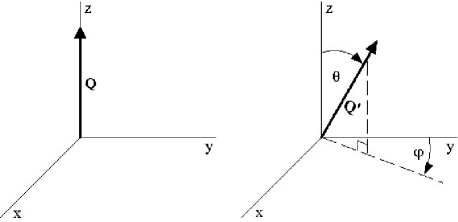
Figure 2: Before initiating the second collision, we rotate the final position and velocity vectors of each SPH particle from the first collision: first by an angle $\theta$ around the $x$-axis and then by an angle $\phi$ around the $z$-axis. The above figure shows how a vector ${\bf Q}$ initially pointing along the $z$-axis is transformed into the new vector ${\bf Q^{\prime}}$ by these rotations.

For the second collision, we want to control the relative orientation of the first collision product’s rotation axis and the orbital plane (or, equivalently, the direction of approach of the third parent star). To do so, we begin with the final state of the first collision and make two rotations to its particle positions and velocities, through the angles $\theta$ and $\phi$. More specifically, the first rotation is clockwise through an angle $\theta$ about the $x$ axis, while the second rotation is clockwise through an angle $\phi$ about the $z$ axis (see Fig. 2). Finally, the particle positions and velocities are uniformly shifted parallel to the $x$-$y$ plane, and the third star is introduced such that the system’s centre of mass will remain at the origin and the periastron positions (in the two body point mass approximation) will occur on the $x$ axis. In order to allow the bulk of the fluid to remain within the gravity grid, the grid is extended up to a full width of $10R_{TO}$ in the $x$ and $y$ directions for some of the second collisions.

We use the same iterative procedure as Lombardi et al. (1996) to determine the bound and unbound mass. SPH structure and composition profiles presented in this paper result from averaging in 100 equally sized bins in the bound mass. Unfortunately, it is extremely difficult to use SPH simulations to specify the equilibrium structure of the outermost few per cent of mass in any collision product. Some SPH particles, although gravitationally bound, are ejected so far from the system’s centre of mass that it would take many dynamical time-scales for them to rain back onto the central product and settle into equilibrium. Our requirement for stopping an SPH calculation is that the entropic variable $A$, when averaged over isodensity surfaces, increases outward over at least the inner 95 per cent of the bound mass in the first collision product, and at least 92 per cent in the second collision product. Many calculations are run longer in order to confirm that no rapid changes are still occurring in the structure and chemical composition distributions.

2.2 Make Me A Star

The results of parabolic collisions between low-mass main-sequence stars can be well explained by simple physical arguments. To a good approximation, the fluid from the parent stars sorts itself such that fluid with the lowest values of $A$ sinks to the core of the collision product while the larger $A$ fluid forms its outer layers. Therefore, the interior structure and the chemical composition profiles of the collision product can be predicted accurately using simple algorithms, instead of hydrodynamic simulations. Based on these ideas, Lombardi et al. (2002) have recently created a publicly available software package, dubbed Make Me A Star (MMAS). This package produces collision product models close to those of an SPH code in considerably less time, while still accounting for shock heating, mass loss, and fluid mixing.

Sorting the shocked fluid according to its entropic variable $A$ gives the $A$ profile of the collision product as a function of the mass $m$ enclosed inside an isodensity surface. In the case of the non-rotating products formed in head-on ($r_{p}=0$) collisions, knowledge of the $A(m)$ profile is sufficient to determine the pressure $P(m)$, density $\rho(m)$, and radius $r(m)$ profiles. Using the $A$ profile determined by sorting, MMAS numerically integrates the equation of hydrostatic equilibrium with $dm=4\pi r^{2}\rho dr$ to determine the $\rho$ and $P$ profiles, which are related through $\rho=(P/A)^{3/5}$. The outer boundary condition is that $P=0$ when $m=M_{MMAS}$, where $M_{MMAS}$ is the desired (gravitationally bound) mass of the collision product. The virial theorem provides a check of the resulting profiles. This approach allows for the quick generation of collision product models, without hydrodynamic simulations, and has already been tested with single-single star collisions.

Presented in this paper are the results from MMAS for triple-star collisions (see §3.2). Our procedure is simple. We call the MMAS routine twice, using the output model from the first collision as one of the input parent models in the second. These MMAS calculations therefore account for the differences in shock heating that arise from changing the order, or the periastron separations, or both, of the collisions. In addition to investigating all of the scenarios considered with the SPH code, we also use MMAS to examine more completely how the sizes of products vary with the periastron separations of the collisions. Furthermore, we include a $0.4{\rm M}_{\odot}$ parent star of radius $0.357{\rm R}_{\odot}$, whose structure is determined by YREC under the same conditions described in §2.1.

For an off-axis collision, knowledge of the specific angular momentum distribution in the collision product is necessary to determine its structure fully, which by itself is a challenging problem (Ostriker & Mark, 1968; Clement, 1978, 1979; Eriguchi & Mueller, 1991; Uryu & Eriguchi, 1995). Although MMAS outputs an approximate specific angular momentum profile of the first collision product, we use only its entropic variable $A(m)$ profile to help initiate the second collision. That is, for one of the parent stars in the second collision, we always give as input to MMAS the structure of a non-rotating star with the desired $A(m)$ profile, a simplification that both eases and quickens computations. The validity of this approximation is supported by the SPH calculations presented in §3.1.3.

Lombardi et al. (2002) implemented version 1.2 of MMAS, while the results of this paper use version 1.6. Besides cosmetic changes, the primary enhancement is that the structure of the collision product is integrated with a Fehlberg fourth-fifth order Runge-Kutta method. In addition, we have fine-tuned the fitted parameter $c_{3}$ from its previous value of -1.1 to the new value -1.0, which has the effect of distributing shocks slightly more uniformly throughout the fluid.

3 Results

Table 1 summarizes five single-single star

Table 1: Summary data of six single-single star collisions.

Case	$M_{1}$	$M_{2}$	$r_{p}$	$T_{f}$	$R_{0.9,SPH}$	$R^{\prime}_{0.9,MMAS}$0	$M_{SPH}$	$M_{MMAS}$
	[${\rm M}_{\odot}$]	[${\rm M}_{\odot}$]	[${\rm R}_{\odot}$]	[hr]	[${\rm R}_{\odot}$]	[${\rm R}_{\odot}$]	[${\rm M}_{\odot}$]	[${\rm M}_{\odot}$]
d	0.8	0.6	0.000	6.24	0.87	0.88	1.304	1.301
e	0.8	0.6	0.368	8.09	1.20	1.24	1.369	1.362
j	0.6	0.6	0.000	6.24	0.91	0.72	1.132	1.121
jk	0.6	0.6	0.123	20.9	1.11	0.79	1.156	1.149
k	0.6	0.6	0.247	27.7	1.52	0.83	1.169	1.162

simulations of parabolic collisions. The table lists: the case name; the masses $M_{1}$ and $M_{2}$ of the parent stars $i=1$ and $2$, respectively; the periastron separation $r_{p}$ of the initial orbit; the stellar time $T_{f}$ when the calculation was terminated; the average radius of the isodensity surface enclosing 90 per cent of the bound mass, as determined by SPH, $R_{0.9,SPH}$, and by MMAS, $R^{\prime}_{0.9,MMAS}$; and the final mass of the collision product as calculated both by SPH, $M_{SPH}$, and by MMAS, $M_{MMAS}$. Previous, higher resolution SPH simulations of cases e and k (see Sills et al., 2001; Lombardi et al., 2002) yield no significant differences from the present calculations. For the cases in Table 1, the mass loss percentage ranges from about 2 to 7 per cent. Comparing the last two columns of this table, we see that the mass loss prescription of MMAS reproduces the SPH results for the final product mass to within 1 per cent in all six cases.

Table 2 summarizes scenarios in which a collision product

Table 2: Summary data of collisions between a third star and a product of a first collision.

Case	First	$M_{3}$	$r_{p,2}$	$\theta$	$\phi$	$T_{f}$	$T/|W|$	$R_{0.9,SPH}$	$R^{\prime}_{0.9,MMAS}$0	$M_{SPH}$	$M_{MMAS}$
	Product	[${\rm M}_{\odot}$]	[${\rm R}_{\odot}$]	[∘]	[∘]	[hr]		[${\rm R}_{\odot}$]	[${\rm R}_{\odot}$]	[${\rm M}_{\odot}$]	[${\rm M}_{\odot}$]
1	d	0.6	0.00	0	0	8.78	0.001	1.2	1.66	1.765	1.747
2	j	0.8	0.00	0	0	15.7	0.001	1.3	1.36	1.769	1.760
3	e	0.6	0.00	0	0	12.0	0.011	1.7	2.31	1.799	1.778
4	e	0.6	0.0955	0	0	12.7	0.059	2.0	3.09	1.851	1.825
5	k	0.8	0.198	0	0	23.1	0.060	2.5	2.05	1.868	1.862
6	k	0.8	0.198	45	0	23.1	0.056	2.4	2.05	1.862	1.862
7	k	0.8	0.00	0	0	21.0	0.005	1.8	1.48	1.794	1.789
8	k	0.8	0.00	90	90	15.7	0.005	1.7	1.48	1.788	1.789
9	k	0.8	0.00	45	90	11.5	0.006	1.7	1.48	1.793	1.789
10	k	0.8	0.00	45	0	15.7	0.006	1.8	1.48	1.794	1.789
11	jk	0.8	0.00	0	0	14.8	0.004	1.5	1.44	1.792	1.781
12	j	0.8	0.505	0	0	23.1	0.077	2.4	2.25	1.883	1.866
13	jk	0.8	0.505	0	0	23.1	0.091	2.9	2.48	1.893	1.890
14	k	0.8	0.505	0	0	23.1	0.092	3.3	2.60	1.893	1.902
15	k	0.8	0.505	90	90	23.1	0.081	3.2	2.60	1.893	1.902
16	k	0.8	0.505	45	90	23.1	0.088	3.3	2.60	1.893	1.902
17	k	0.8	0.505	45	0	23.1	0.090	3.3	2.60	1.895	1.902
18	k	0.8	0.505	90	0	23.1	0.079	3.1	2.60	1.894	1.902
19	k	0.8	0.505	180	0	23.1	0.064	2.7	2.60	1.885	1.902
20	k	0.8	0.758	45	0	39.3	0.091	4.2	2.90	1.912	1.917

from Table 1 (referred to as the first collision product) is collided with a third parent star. The table shows: the case number; the name of the single-single collision that yielded the first collision product; the mass $M_{3}$ of the third ($i=3$) parent star; the periastron separation $r_{p,2}$ of the second collision; the rotation angles $\theta$ and $\phi$ (see Fig. 2); the time $T_{f}$ when the calculation was terminated; the ratio of kinetic to gravitational binding energy $T/|W|$ in the centre-of-mass frame of the final SPH collision product model; the average radius of the isodensity surface enclosing 90 per cent of the bound mass, as calculated by SPH, $R_{0.9,SPH}$, and by MMAS, $R_{0.9,MMAS}$; and the mass of the product as calculated both by SPH, $M_{SPH}$, and by MMAS, $M_{MMAS}$.

All twenty cases presented in Table 2 involve two $0.6{\rm M}_{\odot}$ stars and a single $0.8{\rm M}_{\odot}$ star. If mass loss were neglected completely, the mass of the final collision product would therefore simply be $2.0{\rm M}_{\odot}$. The SPH calculated masses range from about 1.76 to $1.91{\rm M}_{\odot}$, with the largest mass loss occurring for cases with successive head-on collisions.

The cases in Table 2 group naturally together in a variety of ways. Cases 1 and 2 each involve two head-on collisions. Cases 5 and 6 differ only in the orientation of the first collision product’s spin axis, and an identical statement can be made for cases 7 through 10, as well as for cases 14 through 19. Cases 2, 11, and 7 differ only in the periastron separation of the first collision, as do cases 12, 13 and 14. Also, many of the cases differ only in the periastron separation for the second collision: for example, cases 7, 5, and 14, as well as cases 10, 6, 17, and 20.

Even without running an SPH or MMAS calculation, one can generate a “zeroth order” collision product model, valid for all twenty cases, simply by sorting the fluid of the three parent stars by their $A$ values, with $A$ increasing from the core to the surface. In those regions in which more than one parent star contributes, chemical abundances can be determined by an appropriate weighted average: the fraction of fluid with entropic variable in some range $(A,A+\Delta A)$ that originated from any one parent star is just equal to the fluid mass in that same range from that star divided by the total fluid mass in that range from all three stars.

Fig. 3 shows the composition profiles resulting from

Figure 3: Fractional chemical abundances (by mass) versus enclosed mass fraction $m/M$ for a “zeroth order” collision product model generated by sorting the fluid from one $0.8$ and two $0.6{\rm M}_{\odot}$ stars according to their $A$ values, without accounting for mass loss, shock heating or fluid mixing. Here $m$ is the mass enclosed within a surface of constant density and $M$ is the total mass of the collision product, $2.0{\rm M}_{\odot}$ in this model.

this exercise for the merger of two $0.6{\rm M}_{\odot}$ stars and a $0.8{\rm M}_{\odot}$ star, with shock heating, mass loss, and fluid mixing all completely neglected. The innermost 6 per cent and outermost 9 per cent of this collision product model consist of fluid that originated entirely in the $0.8{\rm M}_{\odot}$ parent star, and the profiles there consequently mimic those of the innermost and outermost regions, respectively, of that parent. The profiles in the intermediate region, where all three parent profiles contribute, can be understood by looking back at Fig. 1 and remembering that the smaller $A$ fluid is placed deeper in the product. For example, the C¹³ near $m/M=0.13$ originated in the $0.6{\rm M}_{\odot}$ star, while the higher $A$, C¹³-rich fluid peaked near $m/M=0.5$ originated mostly in the $0.8{\rm M}_{\odot}$ star. Although some of the composition profiles turn out to agree reasonably with our more precise SPH and MMAS calculations, the structure of the star produced by this simple merging procedure does not. In particular, because shock heating is neglected, energy is not conserved during the merger, and the resulting radius for the product is a considerable underestimate. The primary usefulness of the model presented in Fig. 3 is that it serves as a reference to help us evaluate in what ways the shock heating, mass loss, and fluid mixing treated by our SPH and MMAS calculations affect the composition and structure profiles of the collision product.

3.1 Smoothed Particle Hydrodynamics

3.1.1 Varying the collision order

Cases 1 and 2 each involve two consecutive head-on collisions between the same three parent stars. The only variation between these two cases is the order in which the collisions occur: in case 1, the $0.8{\rm M}_{\odot}$ parent is involved in the first collision, while in case 2 it is involved in the second. Fig. 4 shows the resulting chemical composition profiles of the collision products. Because the innermost few per cent of the final collision products consist of low-$A$ fluid that originated in the centre of the $0.8{\rm M}_{\odot}$ parent (see Fig. 5), the composition profiles are nearly identical there. More generally, the resulting profile of each chemical species is at least qualitatively similar throughout the products. The differences in the composition profiles of Fig. 4 are arguably most pronounced for C¹³. In the parent stars, this element exists in appreciable amounts only in a relatively thin shell, and, as shown in Fig. 1, this shell is at a higher value of $A$ in the $0.8{\rm M}_{\odot}$ star than in the $0.6{\rm M}_{\odot}$ star. Exactly where the C¹³-rich fluid is ultimately deposited depends on the details of the shock heating, and hence the order in which the stars collide. In particular, the final C¹³ profile in the case 1 product has two distinct peaks at enclosed mass fractions of $m/M\simeq$ 0.1 and 0.5 (as in our zeroth order model, see Fig 3), whereas the case 2 profile has a single extended peak centred near $m/M$ = 0.2. Fig. 6 displays, as a function of enclosed mass fraction $m/M$ within the product, how each parent contributes to the overall C¹³ profile. The inner peak in the case 1 profile is due mostly to C¹³ that originated in the $0.6{\rm M}_{\odot}$ parent stars, while the outer peak is due mostly to the higher-$A$, C¹³-rich fluid from the $0.8{\rm M}_{\odot}$ parent. In case 2, the $0.8{\rm M}_{\odot}$ star is involved in only the second collision. It therefore experiences less shock heating than in case 1 and more of its fluid is able to penetrate to the core of the final collision product. Consequently, much of the C¹³ from the $0.6{\rm M}_{\odot}$ stars is displaced out to larger enclosed mass fractions, while the C¹³ from the $0.8{\rm M}_{\odot}$ star is shifted inward. The net result is the single extended peak that includes C¹³ from all three parent stars.

Figure 4: Chemical abundance profiles for the case 1 (dashed curve) and case 2 (dotted curve) collision products, as determined by SPH calculations. The chemical abundance fractions are averaged on isodensity surfaces that enclose a mass fraction $m/M$ in the final collision product.

Figure 5: Fractional contribution $f_{i}$ to the mass of the collision product from each parent star as a function of enclosed mass fraction $m/M$ within the product for case 1 (top) and case 2 (bottom), as determined by SPH calculations. Each of these cases involves head-on ($r_{p}=r_{p,2}=0$) collisions among one $0.8$ and two $0.6{\rm M}_{\odot}$ stars; however in case 1 the $0.8{\rm M}_{\odot}$ star is part of the initial collision, whereas in the case 2 scenario it is part of the second collision. Different line types are used for each parent star: $i=1$ (solid curve), $i=2$ (dotted curve), and $i=3$ (dashed curve). Parents with an index $i=1$ or 2 are involved in the first collision, while $i=3$ refers to the third parent star from the second collision. The contribution profile from the $0.8{\rm M}_{\odot}$ parent is labelled in each case.

Figure 6: Fractional abundance of C¹³ versus the enclosed mass fraction $m/M$ in the final collision products of case 1 (dashed curve) and case 2 (dotted curve), as determined by SPH calculations. The top pane shows the total C¹³ abundance. The second pane shows the contribution from the $0.8{\rm M}_{\odot}$ parent, and the bottom two frames show the contribution from the $0.6{\rm M}_{\odot}$ parents, so that the curves in the bottom three panes add up to give the overall profile shown in the top pane.

The detailed differences between the composition profiles of the other elements in Fig. 4 can be understood by considering the $A$ and composition profiles of the parent stars, along with the distribution and amount of shock heating. For example, the core of the $0.8{\rm M}_{\odot}$ parent star is rich in He⁴ and N¹⁴, but depleted of C¹² (see Fig. 1). The lower shock heating to the $0.8{\rm M}_{\odot}$ star in case 2 allows more of its core to sink to the centre of the collision product. Consequently, the He⁴ and N¹⁴ levels are enhanced as compared to case 1, while the C¹² levels are diminished, for final enclosed mass fractions $m/M$ in the range from 0.05 to 0.2.

The mass that is ejected during the collisions comes preferentially from the outer layers of the parent stars, exactly where elements such as Li⁶, Li⁷, and Be⁹ exist. The surface abundances (by mass) in the final case 1 collision product for these three elements are approximately $3\times 10^{-10}$, $4\times 10^{-9}$, and $2\times 10^{-10}$, which is, respectively, about 30, 6, and 3 times less than at the surface of the $0.8{\rm M}_{\odot}$ parent star. In case 2, the surface layers are comparably depleted in these elements: the corresponding abundances are $2\times 10^{-10}$, $6\times 10^{-9}$, and $2\times 10^{-10}$.

The bottom three panes in Fig. 4 show that the distribution of Li⁶, Li⁷, and Be⁹ does differ somewhat between cases 1 and 2. Because the $0.8{\rm M}_{\odot}$ star suffers less shock heating in case 2 than in case 1, it loses less of its mass as ejecta and, consequently, can contribute more Li⁶, Li⁷, and Be⁹ to the outermost layers of the final collision product. Furthermore, when the fluid containing Li⁷ and Be⁹ from the $0.6{\rm M}_{\odot}$ stars is involved in both collisions (case 2), it is shocked more and ultimately either ejected or deposited in the outer $\sim$10 per cent of the product. However in case 1, the one $0.6{\rm M}_{\odot}$ star that is involved in only a single collision can deposit its Li⁷ and Be⁹ of comparatively low-$A$ deeper in the product, resulting in flattened profiles extending further into the interior.

Fig. 5 shows, as a function of $m/M$, the fractional contribution to the final product’s mass from each of the three parent stars for cases 1 and 2, as determined by SPH calculations. In each case, the innermost few per cent of the final collision product consists of low-$A$ fluid that originated in the centre of the $0.8{\rm M}_{\odot}$ parent. Because the first collision in cases 1 and 2 is head-on ($r_{p}=0$), fluid from the first two parent stars is not distributed axisymmetrically in the first collision product (the composition distribution is therefore not axisymmetric, even though the structure of the first product is). In case 2, the $0.8{\rm M}_{\odot}$ star strikes the first collision product on the side with fluid from the first ($i=1$) $0.6{\rm M}_{\odot}$ parent. Fluid from the first $0.6{\rm M}_{\odot}$ parent is therefore heated more than fluid from the second, and the former is buoyed out to larger enclosed mass fractions in the final product. In off-axis collisions, rotation induces shear mixing, so that if two identical stars are involved in the first collision, they contribute essentially equally within the final product: $f_{1}=f_{2}$.

The profiles of Fig. 4 and Fig. 6 demonstrate that the order in which the stars collide can influence shock heating enough to affect, at least slightly, the chemical composition distribution within the final collision product. While the difference in resulting chemical composition profiles is small, Fig. 7 shows that the difference in the structure of the collision product would be completely negligible for most purposes. Although changing the order of these head-on collisions affects how the shock heating is distributed (and hence where any particular fluid element settles), it does not greatly affect the overall amount of heating that occurs nor the amount of mass that is ejected. At least for low Mach number collisions (as with parabolic collisions) that are nearly head-on (so that the merger occurs quickly), shock heating can be thought of as a mild perturbation; consequently, the final $A$ profile, and hence the structure of the final product, is not sensitive to the collision order in such cases.

Figure 7: Structural profiles for the case 1 (dashed curve) and case 2 (dotted curve) collision products, as determined by SPH calculations: the enclosed mass fraction $m/M$, the natural logarithm of the average entropic variable $A$, and the base 10 logarithm of the average density $\rho$, are all plotted as a function of the average distance $r$ from the centre of the collision product to an isodensity surface. Units are cgs.

3.1.2 Varying the direction of approach of the third parent

We now investigate how the direction of approach of the third star toward the first collision product affects the final collision product. One might wonder, for example, whether an impact in the first collision product’s equatorial plane ($\theta=0$ or 180^∘) would yield a qualitatively different result than if the impact had instead occurred on the rotation axis. Cases 5 and 6, cases 7 to 10, and cases 14 to 19 can all be used to examine such effects, as the cases within each set differ only in the angles $\theta$ and $\phi$, by which the first product is rotated (see Fig. 2). We find that while the spin of the final product is of course sensitive to such variations (e.g., see the $T/|W|$ column of Table 2), the composition profiles are nearly unaffected.

Fig. 8 shows the chemical abundance

Figure 8: Chemical abundance profiles for the final collision product of cases 14 (solid curve), 15 (dotted curve), 17 (long dashed curve), and 19 (short dashed curve), as determined by SPH calculations. In these scenarios the same rotating first collision product collides off-axis with a $0.8{\rm M}_{\odot}$ star, with a different orientation of the first collision product’s rotation axis in each case.

profiles of the collision product resulting in four cases in which the angle of approach of the third star is varied (cases 14, 15, 17, and 19). Each of these cases involves an off-axis collision between a case k collision product and a $0.8{\rm M}_{\odot}$ star. In case 14, the first collision product’s spin vector is parallel to the orbital angular momentum of the second collision. In the other cases, the case k collision product is tilted various ways according to the values of $\theta$ and $\phi$ listed in Table 2. In case 19, for example, the case k collision product is flipped over 180^∘ so that it rotates in an opposite direction to that of the case 14 rotation.

In case 14, the fluid of the first product is rotating with the third star’s motion as it impacts ($\theta=0^{\circ}$). Consequently, the merger process is relatively gentle. For larger $\theta$, the relative impact velocity is larger and the merger is somewhat more violent. Cases 14, 17, 15, and 19 have $\theta$ values of 0, 45, 90, and 180^∘, respectively; as $\theta$ increases, slightly less fluid from the $0.8{\rm M}_{\odot}$ star can sink down into the core of the final collision product, and the C¹³ profile rises at a slightly smaller enclosed mass fraction $m/M$ (see Fig. 8). Nevertheless, as shown in Fig. 9, the contribution of each

Figure 9: Fractional contribution $f_{3}$ from the third parent star as a function of enclosed mass fraction $m/M$ within the collision product of cases 14 (solid curve), 15 (dotted curve), 17 (long dashed curve), and 19 (short dashed curve), as determined by SPH calculations. In these scenarios, the first two parent stars are both $0.6{\rm M}_{\odot}$; the third parent star is $0.8{\rm M}_{\odot}$ and approaches from a different angle $\theta$ relative to the rotation of the first collision product in each case. The fractional contribution from each of the first two parent stars is essentially equal and can therefore be determined easily from the $f_{3}$ curve: $f_{1}=f_{2}=(1-f_{3})/2$.

parent star to the product varies very little from case to case. Consequently, the chemical profiles in the collision products also vary little as $\theta$ is changed. Indeed, the He⁴, C¹², N¹⁴, and O¹⁶ profiles in Fig. 8 all look remarkably similar to the corresponding profiles in Fig. 3 for our simple, zeroth order model. However, the C¹³ profile has a single broad peak, for the same reasons as in case 2. Furthermore, because of mass loss, the beryllium and lithium surface abundances are found to be greatly less than our zeroth order model (that neglects mass loss) would indicate.

The structure of the final collision product (see Fig. 10) can be affected by the direction of approach

Figure 10: Structural profiles for the final collision product of cases 14 (solid curve), 15 (dotted curve), 17 (long dashed curve), and 19 (short dashed curve), as determined by SPH calculations. The particular quantities plotted are as in Fig. 7.

for two primary reasons. Firstly, having larger relative velocity at impact leads to larger shock heating. Notice, for example, how the case 19 product has the largest $A$ values in Fig. 10. Secondly, having less angular momentum in the system leads to a more compact product. For example, the case 19 product has the largest enclosed mass fraction for almost any average radius $r$, despite the additional shock heating undergone in this case. Furthermore, by comparing the final masses $M_{SPH}$ listed in Table 2 for the products of cases 5 and 6, of cases 7 through 10, and of cases 14 through 19, one can see that the amount of mass ejected is only very weakly dependent upon the direction of approach of the third parent star, varying by about $0.01{\rm M}_{\odot}$ or less within each of these sets of cases.

3.1.3 Varying the periastron separations of the collisions

We now investigate the effects that the periastron separation of the first collision has on the final collision product. Cases 12, 13, and 14 all involve off-axis collisions with first collision products that are created from the same $0.6{\rm M}_{\odot}$ parent stars but with different periastron separations (cases j, jk, and k, respectively), and hence different inherited angular momenta. Fig. 11 plots the fractional contribution of the third parent star within the merger product.

Figure 11: Fractional contribution of the third parent star, as determined by SPH calculations, within the final collision product for three scenarios that differ only in the periastron separation $r_{p}$ of the first collision: cases 12 (solid curve), 13 (dotted curve), and 14 (dashed curve). In all three cases, the first two parent stars are $0.6{\rm M}_{\odot}$, while the third parent is $0.8{\rm M}_{\odot}$. The $0.8{\rm M}_{\odot}$ parent penetrates into the product the least in case 12, because of the relatively small amount of shock heating suffered by the first product during the first collision in this case.

In all cases, the low-$A$ core of the $0.8{\rm M}_{\odot}$ star is able to sink to the core of the final product. However, as the periastron separation of the first collision is increased, the two $0.6{\rm M}_{\odot}$ parent stars experience more shock heating, and the $0.8{\rm M}_{\odot}$ parent is able to have more fluid penetrate down to the depths near $m/M\sim 0.15$.

Fig. 12 presents chemical composition profiles

Figure 12: Chemical abundance profiles, as determined by SPH calculations, for the final collision product for three scenarios that differ only in the periastron separation $r_{p}$ of the first collision: cases 12 (solid curve), 13 (dotted curve), and 14 (dashed curve).

of the final collision product for these three cases. These profiles demonstrate that the angular momentum of the first collision product has only a small effect on the final collision product. As expected from Fig. 11, the profiles of the three cases are essentially identical in the innermost 5 per cent of the bound mass, because only the core of the $0.8\ {\rm M}_{\odot}$ parent contributes there. The abundance profiles of each chemical species are at least qualitatively, and usually quantitatively, similar throughout the products. The variations that do exist can be understood in terms of the different shock heating during the first collisions. Because the amount of shock heating increases with periastron separation, the case j, jk, and k products have increasingly larger values of $A$ at almost any enclosed mass fraction (this trend is not immediately evident in Fig. 13 only because $\ln A$ is being plotted versus radius and not enclosed mass). The fluid from the $0.8{\rm M}_{\odot}$ star is therefore able to penetrate the case j product the least, the case jk product a little more, and the case k product even more still (see Fig. 11). Consequently the rise in C¹² and C¹³ abundance is pushed out to increasingly larger enclosed mass fractions $m/M$ in Fig. 12 as one considers cases 12, 13, and 14, in that order. In case 12 and arguably case 13, the cases with the lesser amounts of shock heating, traces of two separate peaks are evident in the C¹³ profile. As in our zeroth order model (see Fig. 3), the inner peak is due mostly to C¹³ from the $0.6{\rm M}_{\odot}$ stars while the outer peak is mostly due to C¹³ from the $0.8{\rm M}_{\odot}$ star.

Figure 13: Structural profiles, as determined by SPH calculations, for the final collision product for three scenarios that differ only in the periastron separation $r_{p}$ of the first collision: cases 12 (solid curve), 13 (dotted curve), and 14 (dashed curve). The particular quantities plotted are as in Fig. 7.

Fig. 13 shows that the structure of the bulk of the fluid in the final collision product is not significantly affected by the periastron separation of the first collision, and hence the spin of the first collision product. There is, nevertheless, a visible trend for the enclosed mass fraction at a given average radius to decrease for products with more spin. For example, the isodensity surface with an average radius of $3.2{\rm R}_{\odot}$ encloses about 94 per cent of the case 12 product, about 92 per cent for the case 13 product, and only about 90 per cent of the case 14 product. Such a trend is expected, simply because of expansion due to rotational support.

Cases 10, 17, and 20 can be used to investigate the effects that the periastron separation of the second collision has on the profiles of the final product. Cases 10, 17, and 20 involve collisions between a case k product and a $0.8{\rm M}_{\odot}$ star, with periastron separations for the second collision of $r_{p,2}=0$, 0.505, and $0.758{\rm R}_{\odot}$, respectively, corresponding to a number of passages or interactions $n_{p}=1$, 2, and 3, again respectively. See the discussion of fig. 6 in Lombardi et al. (1996) for the details of how $n_{p}$ is determined.

Fig. 14 reveals the way in which the $0.8{\rm M}_{\odot}$ parent

Figure 14: Fractional contribution of the third parent star, as determined by SPH calculations, within the final collision product for three scenarios that differ only in the periastron separation $r_{p,2}$ of the second collision: cases 10 (solid curve), 17 (dotted curve), and 20 (dashed curve). In all three cases, the first two parent stars are $0.6{\rm M}_{\odot}$, while the third parent is $0.8{\rm M}_{\odot}$. The first collision product results from case k.

contributes to the final product in each of these three cases. As usual, the low-$A$ core of the $0.8{\rm M}_{\odot}$ star sinks to the core of the collision product. As the periastron separation of the second collision is increased, the resulting collision products tend toward larger mass-averaged values of $A$. Fluid from the the $0.8{\rm M}_{\odot}$ star therefore can penetrate the case 10 product the most, the case 17 product a little less, and the case 20 product even less still.

Fig. 15 shows that the composition profiles in these three cases are essentially identical in the innermost few per cent of the collision products. Indeed, the abundance profiles are again at least qualitatively, and usually quantitatively, similar throughout the entire product. As before, slight variations do result from having different distributions of shock heating. In particular, the rise in C¹² and C¹³ abundance is drawn in to smaller enclosed mass fractions $m/M$ in Fig. 15 as one examines cases 10, 17, and 20, in that order. Fig. 16 reveals the differences in the final product structure for these three cases. The top pane shows that the mass distribution of the final product is affected by the periastron separation of the second collision in a way that is simple to understand: increasing the second periastron separation increases both shock heating and rotation, and so a given radius encloses less mass.

Figure 15: Chemical abundance profiles, as determined by SPH calculations, for the final collision product for three scenarios that differ only in the periastron separation $r_{p,2}$ of the second collision: cases 10 (solid curve), 17 (dotted curve), and 20 (dashed curve).

Figure 16: Structural profiles, as determined by SPH calculations, for the final collision product for three scenarios that differ only in the periastron separation $r_{p,2}$ of the second collision: cases 10 (solid curve), 17 (dotted curve), and 20 (dashed curve).

3.2 Fluid sorting with MMAS

3.2.1 Comparison with SPH results

Figure 17: Chemical abundance fractions by mass vs. the enclosed mass fraction $m/M$ in the final collision product for (a) case 1 and (b) case 2. Results both from an SPH simulation (dotted curve) and from the MMAS software package (solid curve) are shown. In each case, both collisions are head-on.

Figure 18: Structure profiles as a function of radius $r$ in the final collision product for (a) case 1 and (b) case 2. Results both from an SPH simulation (dotted curve) and from the MMAS software package (solid curve) are shown. In each case, the final collision product is non-rotating.

In §3.1.2 we found that the direction of approach of the third star only weakly affects the profiles and mass of the final product. We therefore do not account for the angles $\theta$ and $\phi$ of the second collision when applying our fluid sorting package MMAS. As a result, the product model that MMAS generates is identical within each of the following sets: cases 5 and 6, cases 7 through 10, and cases 14 through 19. In all twenty cases presented in Table 2, the final product mass given by MMAS agree with those from SPH to within 1.5 per cent.

Fig. 17 compares the chemical composition profiles of final collision products, as determined by both MMAS and SPH models, for two scenarios (cases 1 and 2) in which each collision is head-on ($r_{p}=r_{p,2}=0$). These cases involve the same three parent stars; however the order in which the stars collide is varied. The MMAS abundance profiles maintain the same qualitative shape as those of the SPH data for almost all of the elements. One possibly important difference is that the MMAS package slightly over-mixes the core in case 1, and, consequently, the central helium abundance is not quite as high as in the SPH calculation. Another noteworthy difference is that the Li⁶ profile, especially in case 1, is not well represented near the surface. Because Li⁶ exists in an even thinner shell at the surface of the $0.8{\rm M}_{\odot}$ star than does Li⁷ and Be⁹, its abundance profile in the product is particularly sensitive to the mass loss distribution during the collisions. Note that MMAS does correctly predict that most Li⁶ is ejected during the collisions. Furthermore, the abundance profiles generated by MMAS much more closely resemble the SPH results than our zeroth order model does (see Fig. 3), indicating that MMAS is capturing the important effects of mass loss and shock heating.

In scenarios such as cases 1 and 2 for which the final product is non-rotating, it is straightforward to obtain the enclosed mass $m$ and density $\rho$ profiles from the $A$ profile by integrating the equation of hydrostatic equilibrium (see §2.2). Fig. 18 shows the resulting structure of the final collision products. The kink in the $A$ profile a little inside $r=0.1{\rm R}_{\odot}$ marks the boundary within which fluid from only the $0.8{\rm M}_{\odot}$ star contributes, and MMAS reproduces this feature quite well. The central density of the SPH model is slightly less than that of the MMAS model, mostly due to how density is calculated as a smoothed average in SPH. Despite this difference, the overall structure of the collision product is extremely well reproduced by MMAS.

Fig. 19 compares the chemical composition profiles for SPH and MMAS data for case 4, a situation in which both collisions are off-axis. The most noticeable discrepancies are that MMAS again slightly over-mixes the core and underestimates the surface Li⁶ abundance. Nevertheless, the chemical abundance profiles produced by the MMAS package and the SPH code are extremely similar. For example, MMAS correctly reproduces the C¹³ abundance, with three peaks each corresponding to a different parent star. The inner peak is due to the low-$A$ fluid from the $0.6{\rm M}_{\odot}$ star involved in only the second collision, the middle peak represents fluid from the other $0.6{\rm M}_{\odot}$ star, and the outer peak represents high-$A$ fluid from the $0.8{\rm M}_{\odot}$ parent (see Fig. 20).

Figure 19: Chemical abundance fraction by mass versus the enclosed mass fraction $m/M$ in the final collision product for both the MMAS (solid curve) and the SPH (dotted curve) data of the case 4 collision product.

Figure 20: Fractional abundance of C¹³ versus the enclosed mass fraction $m/M$ in the final case 4 collision product, as determined both by MMAS (solid curve) and by SPH (dotted curve). The top pane shows the total C¹³ abundance, while the bottom three panes show the contributions from each individual parent star: C${}^{13}_{1}$ is the contribution from the $0.8{\rm M}_{\odot}$ parent, C${}^{13}_{2}$ is the contribution from the $0.6{\rm M}_{\odot}$ parent in the first collision, and C${}^{13}_{3}$ is the contribution from the $0.6{\rm M}_{\odot}$ parent in the second collision.

Note that this feature is reproducible by MMAS only because it accounts for shock heating in each collision (compare to our zeroth order model of Fig. 3, in which there are only two peaks in the C¹³ profile).

In many of the MMAS models, small kinks, or discontinuities, are evident in some of the abundance profiles: such features mark locations outside of which an additional parent star either starts or stops contributing. For example, in the case 5 and 6 collision product, a kink exists in the C¹² and C¹³ profiles near $m/M=0.08$ (see Fig. 21). As is evident from Fig. 22, fluid inside of the

Figure 21: Chemical abundance fraction by mass versus the enclosed mass fraction $m/M$ in the final collision product for both the MMAS (solid curve) and the SPH data of the case 5 (dotted curve) and case 6 (dashed curve) collision products. Note that our MMAS results do not distinguish between cases 5 and 6, as they differ only in the orientation of the first product’s spin.

Figure 22: Fractional contribution $f_{i}$ of each parent star $i$ versus the enclosed mass fraction $m/M$ in the case 5 and 6 collision products, as determined both by MMAS (solid curve) and by SPH. The dotted curve corresponds to the case 5 SPH results, while the dashed curve gives the case 6 SPH results. The same MMAS model is valid for both cases, as they differ only in the direction of the first product’s rotation axis. The $i=1$ and 2 parents are $0.6{\rm M}_{\odot}$, while the $i=3$ parent is $0.8{\rm M}_{\odot}$.

$m/M\approx 0.08$ shell originated solely in the $0.8{\rm M}_{\odot}$ parent star. In the range $m/M\ga 0.08$, all three parent stars contribute. The smoothing that is inherent to the SPH scheme makes it difficult to resolve such features with our hydrodynamics code. It is possible that similarly abrupt changes in abundance could occur in nature within real collision products.

By comparing the SPH data within Fig. 21, as well as within Fig. 22, we also see an example of the trend discussed in §3.1.2. Namely, the direction of the first collision product’s rotation axis (or equivalently the direction of approach of the third parent) has little effect on the final collision product. Indeed, when using MMAS, our approach is to neglect completely the rotation of the first collision product, which is why the same MMAS model applies to both cases 5 and 6.

Figure 23: Entropic variable $A$ as a function of enclosed mass fraction $m/M$ in representative final collision products. In frame (a), the same MMAS model (solid curve) is compared against our SPH models for cases 18 (dotted curve) and 19 (dashed curve): our implementation of MMAS does not distinguish between these cases, as they differ only in the orientation of the first collision product’s rotation axis. In frame (b), the MMAS (solid curve) and SPH (dashed curve) results are compared for case 20. The MMAS profiles have the same qualitative form as the SPH results, except in the outer $\sim 10$ per cent of the bound mass where the SPH models have not settled into equilibrium.

Fig. 23 plots the entropic variable $A$ versus the enclosed mass fraction for the final collision products of cases 18, 19, and 20, as determined both by SPH and MMAS. Cases 18 and 19 differ only in the direction of approach of the third star, and we again see that this variation has little effect on the SPH results. The kink in all of the profiles slightly inside $m/M=0.1$ marks the boundary within which fluid from only the $0.8{\rm M}_{\odot}$ star contributes. MMAS again reproduces this feature quite well. MMAS does underestimate the shock heating to the core and hence the central value of $A$, although some of this discrepancy is due to the spurious heating evident in longer SPH simulations (Lombardi et al., 1999). Nevertheless, it is likely that this difference between the MMAS and SPH models would last only as a transient during the thermal relaxation in a stellar evolution calculation. It is also worth noting that, while the SPH calculations need to be terminated before all of the bound fluid can settle into equilibrium (see §2.1), the MMAS $A$ profile does steadily increase outward throughout the entire product.

3.2.2 Sizes of collision products

Unfortunately it is a difficult task to determine the overall size of a collision product, either with SPH simulations or with a package like MMAS. Whenever there is any mass loss in an SPH simulation, there will also be SPH particles that are nearly unbound and, in practice, still moving away from the product when the simulation is terminated. These particles would ultimately form the outermost layers of the collision product, but it would take an utterly unfeasible amount of time to wait for them to come back and settle into equilibrium.

The entropic variable $A$ profile produced by MMAS seems quite reasonable, both because it increases all the way out to the surface and because the SPH results tend to approach its form as more of the fluid settles into equilibrium. However, there are no simulation data to compare against for the very outermost layers of a product and so the exact form of the profile there is difficult to validate. Not surprisingly, the radius of the collision product is rather sensitive to the $A$ profile. For example, simply by changing the parameter $c_{3}$ from -1.0 to the still very reasonable value of -1.1, which tends to distribute slightly more shock heating to the outer layers (see Lombardi et al., 2002), the radii of our MMAS final collision product models for case 1 and for case 2 increase by about a factor of 2. Despite such uncertainties, it is still interesting to get a crude estimate of the sizes of the collision products immediately from MMAS. In making these estimates, we do not account for the expansion due to rotation, but instead simply integrate the equation of hydrostatic equilibrium for a non-rotating star with the same $A$ profile, using the outer boundary condition that the pressure vanishes. The radii calculated therefore represent the sizes that the products would have if some mechanism were to brake their rotation without disturbing their $A$ profiles.

Fig. 24 plots the radii at various enclosed mass fractions for

Figure 24: As a function of the normalized periastron separation $r_{p}/(R_{1}+R_{2})$, each pane shows the radius $R^{\prime}$ that encloses, from the top curve to the bottom one, 100, 99, 95, 86, and 50 per cent of the total bound mass of the collision product, on a logarithmic scale and as determined by MMAS. The scale on the left gives the radius in solar units, while the scale on the right normalizes the radius to the sum of the parent star radii. The combination of parent stars considered are (a) 0.8 and $0.8{\rm M}_{\odot}$, (b) 0.6 and $0.6{\rm M}_{\odot}$, (c) 0.4 and $0.4{\rm M}_{\odot}$, (d) 0.8 and $0.6{\rm M}_{\odot}$, (e) 0.8 and $0.4{\rm M}_{\odot}$, and (f) 0.6 and $0.4{\rm M}_{\odot}$.

products generated in single-single star collisions involving 0.4, 0.6 and $0.8{\rm M}_{\odot}$ parent stars, as determined by MMAS. These radii are plotted against the normalized periastron separation $r_{p}/(R_{1}+R_{2})$, which we allow to exceed unity slightly to account for bulges in the parent stars. The general trend is that as the periastron separation increases, the collisions are more long-lived, there is more shock heating, and the radii of the collision products increase. Because the fluid in the deep interior of the product is largely shielded from shocks, the $A$ profile there, and hence the radius $r$ profile, are not too strongly dependent on the periastron separation of the collision. As a result, the radii versus periastron separation curves of Fig. 24 become closer to horizontal as one looks to smaller enclosed mass fraction. For the cases examined in Fig. 24, the full (100 per cent enclosed mass) radius of the collision product is always at least about twice the sum of the radii of the parent stars, and often even much larger than this. For example, if two $0.8{\rm M}_{\odot}$ stars suffer a grazing ($r_{p}\approx R_{1}+R_{2}$) collision, the collision product then has a full radius of about $40{\rm R}_{\odot}$, about 20 times larger than the sum $R_{1}+R_{2}$ of the parent star radii. We therefore expect that the collisional cross-section of these first products will be significantly enhanced over that of their thermally relaxed counterparts.

Fig. 25 is similar to Fig. 24, but for triple-star

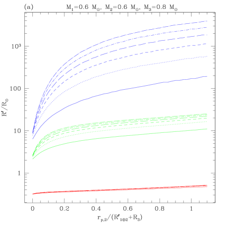
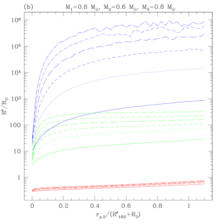
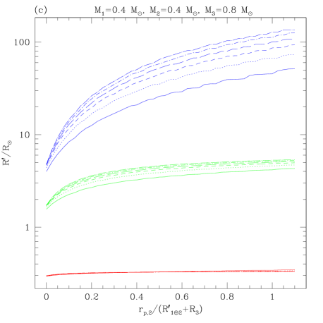
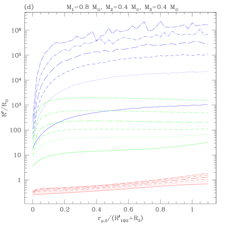
Figure 25: We plot various radii $R^{\prime}$ of the final collision product (as determined by MMAS) as a function of the periastron separation of the second collision, normalized to sum of the radii of the colliding stars. The radius $R^{\prime}_{1\oplus 2}$ of the first collision product is the 100 per cent radius from Fig. 24 corresponding to various normalized periastron separations for the first collision: $r_{p,1}/(R_{1}+R_{2})=0$ (solid curve), 0.2 (dotted curve), 0.4 (short dashed curve), 0.6 (long dashed curve), 0.8 (dot - short dashed curve), and 1.0 (dot - long dashed curve). There are three curves of each line type: the bottom one corresponds to the radius enclosing 50 per cent of the final bound mass, the middle one corresponds to the 95 per cent radius, and the top one to the 100 per cent radius.

collisions. We use different line types to represent various normalized periastron separations $r_{p}/(R_{1}+R_{2})$ for the first collision, and along the horizontal axis we vary the normalized periastron of the second collision. The curves give the radii at three different enclosed mass fractions. For each of the six $r_{p}$ values in a frame of Fig. 25, we performed a nested loop over 45 equally spaced values of the normalized periastron separation for the second collision, from 0 to 1.1. Therefore, MMAS treated 270 different triple-star collisions (in a few minutes on a Pentium IV workstation) for each of the four plots. Note that there is a general trend for the radius of the collision product to increase as the first periastron separation increases, as expected; this effect is mild for the 50 per cent enclosed mass radius, and rather dramatic for the full radius. Even more significant is the second periastron separation, with grazing second collisions resulting in products that are substantially larger than those from head-on collisions: the shock heating suffered by the already diffuse outer layers of the first collision product is severe when multiple pericentre passages occur before merger. Once $r_{p,2}$ grows large enough for the third star’s initial impact to be outside of the first product’s core, so that more than one pericentre passage would result before merger, then the shock heating is no longer as sensitive to $r_{p,2}$ and the full radius surfaces in Fig. 25 tend to plateau. How strongly the full radius varies with the $r_{p,2}$ therefore depends on the mass distribution within the first product. For first products with a more uniform density, such as in the product of two $0.4{\rm M}_{\odot}$ stars, the final product size increases more gradually and consistently with $r_{p,2}$.

As the mass of any one of the three parent stars is increased, the trend is for the radius of the collision product to increase as well. For example, Fig. 25(a) shows that for collisions in which two $0.6{\rm M}_{\odot}$ stars collide and then a $0.8{\rm M}_{\odot}$ collides with the first product, the final collision product radius does not exceed a few times $10^{3}{\rm R}_{\odot}$. If one of the $0.6{\rm M}_{\odot}$ stars is substituted with a $0.8{\rm M}_{\odot}$ star, then the final radius can be as large as about $10^{6}{\rm R}_{\odot}$ [see Fig. 25(b)]. This extreme size is due to the phenomenally diffuse outer layers of the product: the average density of such a star is only $\sim 10^{-18}$ g cm^-3. The noise visible on some of the full radius curves is due to approaching the limiting numerical precision during the structure integration in these diffuse regions.

From Fig. 25 we see that the radius that encloses 95 per cent of the total mass, while still large, is often orders of magnitude smaller than the full radius of the final product. Because of the low densities involved, the full radius calculated is rather sensitive to the details of the shock heating during the collision. Changing the MMAS parameter $c_{3}$ from -1.0 to -1.1, for example, can increase the full radius by a factor of a few, although the radius enclosing 50 per cent of the total mass does not change by more than a few per cent. Nevertheless, any reasonable form and amount of shock heating yields products that are significantly larger than a thermally relaxed star with the same mass and composition.

Colliding the same three parent stars in a different order does not drastically affect the mass of the final product, although it does significantly affect its size. Consider, for example, frames (c) and (d) of Fig. 25. If two $0.4{\rm M}_{\odot}$ stars collide and then the resulting product collides with a $0.8{\rm M}_{\odot}$ star, the final product typically has a radius of order $\sim 10-100{\rm R}_{\odot}$, but if the $0.8{\rm M}_{\odot}$ star is switched into the first collision instead, the final radius is usually in the range from $\sim 100-10^{6}{\rm R}_{\odot}$. The primary reason for this difference is that a collision between the 0.4 and $0.8{\rm M}_{\odot}$ stars yields a product with especially diffuse outer layers, and, as a result, is subject to a larger number of passages and hence more shock heating during a second collision.

4 Discussion

4.1 Concluding remarks

We have used SPH and the software package MMAS to study triple-star collisions. Although such collisions span a tremendous amount of parameter space, our modest number of SPH calculations do provide some valuable insights. For the (parabolic) encounters that we consider, we find that the order in which stars collide (see §3.1.1), the angle of approach of the third star (§3.1.2), and the periastron separation of the collisions (§3.1.3) have only a slight effect on the chemical composition distribution within the final collision product. The order and orbital parameters of the collisions can, however, significantly affect the size and structure of the product.

The results of §3.2.1 help establish that the simple fluid sorting algorithm of MMAS reproduce the important features of our SPH models, even when one of the parent stars is itself a collision product. The MMAS package can therefore be considered an adequate, if not an accurate, substitute for a hydrodynamics code in many situations. This realization will help simplify the process of generating collision product models in cluster simulations, because a full hydrodynamics calculation will not necessarily need to be run for each collision. Indeed, we hope the MMAS package will be used to help account for stellar collisions in dynamics simulations of globular clusters. Toward this end, MMAS is already being incorporated into two software packages, TRIPTYCH and TRIPLETYCH, that respectively treat encounters between two stars and among three stars (see Sills et al., 2003). These packages are controlled through a web interface and treat the orbital trajectories, possible merger(s), and evolution of the merger product and therefore incorporate three main branches of stellar astrophysics: dynamics, hydrodynamics, and evolution.

The product size estimates of §3.2.2 are admittedly crude. For example, partial ionization and radiation pressure are neglected. Although the exact size of a collision product is difficult to determine, our calculations indicate that the first and final collision products are always significantly larger than their thermally relaxed counterparts would be. Indeed, according to our MMAS calculations in §3.2.2, the final collision product can have a radius up to $\sim 10^{6}{\rm R}_{\odot}$, easily exceeding the size of a typical red giant. Furthermore, these calculations have assumed that some mechanism has braked the often rapid rotation of the products, so any rotation that does remain will only further enhance the size of the products. The extended sizes of the products will increase the multi-star collision rate over that calculated in previous treatments of binary-single and binary-binary encounters.

All of the scenarios we consider with SPH in this paper involve one $0.8$ and two $0.6{\rm M}_{\odot}$ stars. Without shock heating, the low-$A$ fluid of the $0.8{\rm M}_{\odot}$ star would sink to the core of the final collision product, while its high-$A$ portions of the $0.8{\rm M}_{\odot}$ would settle in the outer layers. The intermediate layers of the product would consist of fluid with the same $A$ range from all the parents. Simply sorting the fluid in this way, without running a hydrodynamics calculation, can therefore provide a zeroth-order model of the collision product that captures some of its important qualitative features (see Fig. 3).

However, non-uniform shock heating during the collisions somewhat alters the relative values of the entropic variable $A$ in the fluid, resulting in a slightly different sorting pattern. Because the amount and distribution of shock heating are dependent on the details of a collision, the sorting of the fluid varies with, for example, the order in which the stars collide. Shock heating can have larger consequences on the chemical abundance profiles of elements, such as C¹³, that exist in substantial amounts only in a small shell in the initial parent stars. However, the chemical abundance profiles of most elements, particularly helium, are always qualitatively the same, regardless of how the three stars are merged. Because the abundance and distribution of helium (and hence hydrogen) is one of the most important factors in determining the collision product’s subsequent course of stellar evolution, we believe that the order and geometry of the collisions will not significantly affect the stellar evolution of the product. Indeed, Sills et al. (2002) have recently presented a set of stellar evolution calculations for a collision product for which the starting YREC models were generated from SPH calculations of different resolutions. The variations in the initial helium profiles of their models are roughly comparable to those in our helium profiles resulting from colliding three parent stars in different ways. Although Sills et al. (2002) do find detailed differences in the evolution, especially during the “pre-main-sequence” contraction, the evolutionary tracks and time-scales are quite similar. We therefore feel that, for low-velocity collisions, the hydrodynamical details of how three stars are merged will not significantly affect the stellar evolution of the collision product—the major caveat here being that the geometry of the collisions can of course affect the rotation of the product, which in turn can greatly affect its evolution (Sills et al., 2001).

Surface abundances of lithium and beryllium are particularly interesting to monitor, as these elements can be used as observational indicators of mixing and perhaps collisional history. As in the single-single star collisions presented by Lombardi et al. (2002), we find that the triple-star mergers presented here yield collision products that are severely depleted of lithium and somewhat of beryllium at the surface. Even in the relatively gentle (parabolic) cases that we have considered, the collisions are energetic enough to expel most of the lithium and beryllium from the outer layers of the parents.

4.2 Future work

There are many scenarios to explore when dealing with collisions in environments as chaotic as dense stellar systems. Different orbital geometries besides the parabolic trajectories treated in this paper still need to be considered in more detail. Large stellar velocities in galactic nuclei lead to hyperbolic collisions. In globular clusters, perturbations to a binary can lead to an elliptical collision, while an encounter with a very hard binary can lead to significantly hyperbolic collisions.

Future studies may want to include a more detailed look at the hydrodynamics during grazing encounters, which could be done efficiently with the help of GRAPE (short for GRAvity PipE) special purpose hardware for calculating the self-gravity of the system. Furthermore, encounters involving more than three stars, such as in binary-binary interactions, may also warrant further examination: for example, the final collision product generated in a triple-star merger is typically so extended that it could immediately start suffering Roche lobe overflow if left in orbit around a fourth star.

Collisions among a larger variety of stellar types and masses, reflective of the diverse populations of clusters, will also need to be explored. We have been concentrating on low-mass main-sequence stars, but collisions between high-mass main-sequence stars in young compact star clusters, or giants located in the dense cores of globular clusters, for example, are frequent. A logical first step would be to examine high-mass main-sequence stars in a runaway merger scenario. It would therefore be very useful to develop a generalization of the fluid sorting method that includes radiation pressure in the equation of state.

Due to shock heating during the collision, the product is much larger than a thermally equilibrated main-sequence star of the same mass. How much of an effect this increased radius has on the effective cross section for merger is subject to many variables, including the structure of the product’s outer layers and the velocity of approaching stars. In environments such as active galactic nuclei, where relative velocities tend to be high, the low-density outer layers of a newly formed collision product could likely get stripped by passing stars. However, in globular clusters, where stellar velocities tend to be small, collisions with even low-density envelopes may lead to significantly increased rates of merger. It would be useful to develop a robust collision module that could quickly predict whether any given collision trajectory will lead to a merger, and, if not, describe how the stars are affected by the interaction.

One simple approximation often implemented in cluster simulations is that a collision product instantaneously achieves its thermally relaxed radius, a good approximation when the time between collisions is much longer than the thermal time-scale. Arguing instead that the global thermal time-scale of the first product can be much larger than the time between collisions in interactions involving binaries, we make a different approximation in this paper, namely that the first product’s radius (and more generally its structure) does not substantially evolve between collisions. Future scattering experiments could model thermally relaxing stars and study more carefully the timescale between collisions mediated by binaries. The thermal time-scale in the outer layers of a collision product can be orders of magnitude less than its global thermal time-scale (see table 1 of Sills et al., 1997), so that it may actually be necessary to follow the thermal contraction and stellar orbits simultaneously. Indeed, in the extremely low density layers of a collision product, it is even possible for the thermal time-scale to be comparable to the (hydro)dynamical time-scale, so that the product could undergo significant thermal contraction even before it reaches hydrodynamical equilibrium. It would be helpful if future stellar evolution calculations of collision products included a detailed description of the products’ size and structure throughout the thermal relaxation stage. How quickly the outer layers of the thermally expanded product change with time will substantially affect its likelihood of subsequent collisions. Initial conditions for such stellar evolution calculations could be provided by the publicly available MMAS package.

The primary hurdle for incorporating collisions into realistic stellar dynamics simulations is currently the stellar evolution of the collision products. Such stars are highly non-canonical, typically with very peculiar structural and composition profiles, and present a challenging set of initial conditions for stellar evolution codes. To make matters even more intricate, rotation, which is typically rapid after merging, will affect the structural properties and chemical compositions of the stars as they evolve (e.g., Sills et al., 2001). This rapid rotation also has the effect of ejecting mass as the product thermally contracts. Studying this emitted mass will be worthwhile, as it may likely carry away angular momentum and at least partially brake rotating collision products.

References

- Aarseth (1999) Aarseth S. J., 1999, PASP, 111, 1333
- Bacon, Sigurdsson, & Davies (1996) Bacon D., Sigurdsson S., Davies M. B., 1996, MNRAS, 281, 830
- Bailyn (1995) Bailyn C. D., 1995, ARA&A, 33, 133
- Balsara (1995) Balsara D., 1995, J. Comput. Phys., 121, 357
- Baumgardt et al. (2003) Baumgardt H., Hut P., Makino J., McMillan S. L. W., Portegies Zwart S. F., 2003, ApJ (Letters), in press
- Benz & Hills (1987) Benz W., Hills J. G., 1987, ApJ, 389, 546
- Cleary & Monaghan (1990) Cleary P. W., Monaghan J. J., 1990, ApJ, 349, 150
- Clement (1978) Clement M. J., 1978, ApJ, 222, 967
- Clement (1979) Clement M. J., 1979, ApJ, 230, 230
- Davies, Benz & Hills (1994) Davies M. B., Benz W., Hills J. G., 1994, ApJ, 424, 870
- Eriguchi & Mueller (1991) Eriguchi Y., Mueller E., 1991, A&A, 248, 435
- Freitag & Benz (2002) Freitag M., Benz W., 2002, A&A, 394, 345
- Freitag & Benz (2003) Freitag M., Benz W., 2003, in Shara M. M., ed., ASP Conf. Ser. Vol. 263, Stellar Collisions, Mergers and Their Consequences, p. 261
- Gerssen et al. (2002) Gerssen J., van der Marel R. P., Gebhardt K., Guhathakurta P., Peterson R. C., Pryor C., 2002, AJ, 124, 3270
- Gerssen et al. (2003) Gerssen J., van der Marel R. P., Gebhardt K., Guhathakurta P., Peterson R. C., Pryor C., 2003, AJ, 125, 376
- Giersz (2001) Giersz M., 2001, MNRAS, 324, 218
- Giersz & Spurzem (2003) Giersz M., Spurzem R., 2003, submitted to MNRAS (astro-ph/0301643)
- Gingold & Monaghan (1977) Gingold R. A., Monaghan J. J., 1977, MNRAS, 181, 375
- Goodman & Hernquist (1991) Goodman J., Hernquist L., 1991, ApJ, 378, 637
- Heggie (1975) Heggie D. C., 1975, MNRAS, 173, 729
- Heggie & Hut (2003) Heggie D., Hut P., 2003, The Gravitational Million-Body Problem, Cambridge University Press: Cambridge
- Hockney & Eastwood (1988) Hockney R. W., Eastwood J. W., 1988, Computer Simulation Using Particles, Bristol: Hilger
- Hurley, Pols, & Tout (2000) Hurley J. R., Pols, O. R., Tout C. A., 2000, MNRAS, 315, 543
- Hurley & Shara (2002) Hurley J. R., Shara M. M., 2002, ApJ, 570, 184
- Hurley et al. (2001) Hurley J. R., Tout C. A., Aarseth, S. J., Pols O. R., 2001, MNRAS, 323, 630
- Hurley, Tout, & Pols (2002) Hurley J. R., Tout C. A., Pols O. R., 2002, MNRAS, 329, 897
- Hut et al. (1992) Hut P. et al., 1992, PASP, 104, 981
- Hut et al. (2003) Hut P. et al., 2003, New Astronomy, 8, 337.
- Joshi, Nave, & Rasio (2001) Joshi K. J., Nave C. P., Rasio F. A., 2001, ApJ, 550, 691
- Joshi, Rasio, & Portegies Zwart (2000) Joshi K. J., Rasio F. A., Portegies Zwart S. F., 2000, ApJ, 540, 969
- Lai, Rasio & Shapiro (1993) Lai D., Rasio F. A., Shapiro S. L., 1993, ApJ, 412, 593
- Lombardi et al. (1996) Lombardi J. C., Rasio F. A., Shapiro S. L., 1996, ApJ, 468, 797
- Lombardi et al. (1999) Lombardi J. C., Sills A., Rasio F. A., Shapiro S. L., 1999, J. Comput. Phys., 152, 687
- Lombardi et al. (2002) Lombardi J. C., Warren J. S., Rasio F. A., Sills A., Warren A. R., 2002, ApJ, 568, 939
- Lucy (1977) Lucy L. B., 1977, AJ, 82, 1013
- McMillan & Hut (1996) McMillan S. L. W., Hut P., 1996, ApJ, 467, 348.
- Meylan & Heggie (1997) Meylan G., Heggie D. C., 1997, A&ARv, 8, 1
- Monaghan (1992) Monaghan J. J., 1992, ARA&A, 30, 543
- Ostriker & Mark (1968) Ostriker J. P., Mark J. W.-K., 1968, ApJ, 151, 1075
- Ouellette & Pritchet (1998) Ouellette J. A., Pritchet C. J., 1998, AJ, 115, 2539
- Portegies et al. (1997) Portegies Zwart S. F., Hut P., McMillan S. L. W., Verbunt F., 1997, A&A, 328, 143
- Portegies et al. (1997) Portegies Zwart S. F., Hut P., Verbunt F., 1997, A&A, 328, 130
- Portegies Zwart & McMillan (2002) Portegies Zwart S. F., McMillan S. L. W., 2002, ApJ, 576, 899
- Portegies Zwart et al. (1999) Portegies Zwart S. F., Makino J., McMillan S. L. W., Hut P., 1999, A&A, 348, 117
- Portegies Zwart et al. (2001) Portegies Zwart S. F., McMillan S. L. W., Hut P., Makino J., 2001, MNRAS, 321, 199
- Portegies Zwart & Verbunt (1996) Portegies Zwart S. F., Verbunt F. W. M., 1996, A&A, 309, 179
- Quinlan & Shapiro (1990) Quinlan G. D., Shapiro S. L., 1990, ApJ, 356, 483
- Rasio (1991) Rasio F. A., 1991, PhD thesis, Cornell Univ.
- Rasio & Livio (1996) Rasio F. A., Livio M., 1996, ApJ, 471, 366
- Rasio & Lombardi (1999) Rasio F. A., Lombardi, J. C., 1999, JCAM, 109, 213
- Rasio, Freitag, & Gürkan (2003) Rasio F. A., Freitag M., Gürkan M. A., 2003, to appear in “Carnegie Observatories Astrophysics Series, Vol. 1: Coevolution of Black Holes and Galaxies,” ed. L. C. Ho, Cambridge: Cambridge Univ. Press, astro-ph/0304038
- Rasio & Shapiro (1991) Rasio F. A., Shapiro S. L., 1991, ApJ, 377, 559
- Rasio & Shapiro (1992) Rasio F. A., Shapiro S. L., 1992, ApJ, 401, 226
- Rasio & Shapiro (1994) Rasio F. A., Shapiro S. L., 1994, ApJ, 432, 242
- Rubenstein & Bailyn (1997) Rubenstein E. P., Bailyn C. D., 1997, ApJ, 474, 701
- Sandquist et al. (1997) Sandquist E. L., Bolte M., Hernquist L., 1997, ApJ, 477, 335
- Sandquist et al. (2000) Sandquist E. L., Taam R. E., Burkert A., 2000, ApJ, 533, 984
- Sandquist et al. (1998) Sandquist E. L., Taam R. E., Chen X., Bodenheimer P., Burkert A., 1998, ApJ, 500, 909
- Shara (2002) Shara M. M., 2002, Scientific American, November, 44
- Shara & Hurley (2002) Shara M. M., Hurley J. R., 2002, ApJ, 571, 830
- Sills et al. (2003) Sills A. et al., 2003, New Astronomy, in press (astro-ph/0301478)
- Sills et al. (2002) Sills A., Adams T., Davies M. B., Bate M. R., 2002, MNRAS, 332, 49
- Sills et al. (2001) Sills A., Faber J. A., Lombardi J. C., Rasio F. A., Warren A. R., 2001, ApJ, 548, 323
- Sills & Lombardi (1997) Sills A., Lombardi J. C., 1997, ApJ, 484, L51
- Sills et al. (1997) Sills A., Lombardi J. C., Bailyn C. D., Demarque P., Rasio F. A., Shapiro S. L., 1997, ApJ, 487, 290
- Springel & Hernquist (2002) Springel V., Hernquist L., 2002, MNRAS, 333, 649
- Spurzem & Takahashi (1995) Spurzem R., Takahashi K., 1995, MNRAS, 272, 772
- Takahashi & Portegies Zwart (2000) Takahashi K., Portegies Zwart S. F., 2000, ApJ, 535, 759
- Terman et al. (1994) Terman J. L., Taam R. E., Hernquist L., 1994, ApJ, 422, 729
- Terman et al. (1995) Terman J. L., Taam R. E., Hernquist L., 1995, ApJ, 445, 367
- Uryu & Eriguchi (1995) Uryu K., Eriguchi Y., 1995, MNRAS, 277, 1411
- Vesperini & Chernoff (1994) Vesperini E., Chernoff D. F., 1994, ApJ, 431, 231
- Watters et al. (2000) Watters W. A., Joshi K. J., Rasio F. A., 2000, ApJ, 539, 331
- Young et al. (2001) Young P. A., Mamajek E. E., Arnett D., Liebert J., 2001, ApJ, 556, 230