Introducing EMILI: Computer Aided Emission Line Identification

Abstract

The identification of spectral lines can be a tedious process requiring the interrogation of large spectroscopic databases, but it does lend itself to software algorithms that can determine the characteristics of candidate line identifications. We present here criteria used for the identification of lines and a logic developed for a line identification software package called EMILI, which uses the v2.04 Atomic Line List as the basic line database. EMILI considers all possible database transitions within the wavelength uncertainties for observed optical emission lines and computes an approximate intensity for each candidate line. It searches for other multiplet members that are expected to be seen with each candidate line, and rank orders all of the tentative line identifications for each observed line based on a set of criteria. When applied to the spectra of the Orion Nebula and the planetary nebula IC 418, EMILI’s recommended line ID’s agree well with those of previous traditional manual line assignments. The existence of a semi-automated procedure should give impetus to the study of very high signal-to-noise spectra, enabling the identification of previously unidentified spectral lines to be handled with ease and consistency.

1 Line Identification In Rich Emission-Line Spectra

Correct identification of spectral lines is fundamental to all spectroscopic analyses. For lines commonly observed in astronomical spectra, a century of study has resulted in agreement on those transitions that give rise to the stronger lines observed at visible wavelengths. However, there is still uncertainty about the proper identification of many lines, and this problem is even more severe in other wavelength regions. As spectra achieve fainter detection limits, the increasing number of transitions observed leads to a larger fraction of uncertain identifications. The effort involved in making correct line identifications for the large numbers of lines detected in high signal-to-noise (S/N) spectra can be daunting, especially since identifications must be made on the basis of overall astrophysical consistency, causing correct line identifications to be mutually interdependent. This problem has been studied in the past for stellar absorption spectra, and techniques have been developed for distinguishing between chance coincidences and true identifications (Hartoog, Cowley, & Cowley, 1973; Cowley & Adelman, 1990).

Line identification is often problematic for emission-line objects because, unlike absorption lines which are usually formed near conditions of thermodynamic equilibrium, emission lines are formed under conditions where coincidental resonances and unusual excitation mechanisms cause isolated individual transitions to have strengths that deviate from their equilibrium values by many orders of magnitude. The difficulty in making correct identifications for the large numbers of faint lines observed in emission spectra has acted as a disincentive to obtain the very high signal-to-noise spectra that are necessary for their detection. However, deep high resolution spectra of both H II regions (Esteban et al., 1998, 1999; Baldwin et al., 2000) and planetary nebulae (Liu et al., 1995, 2000) are now becoming routinely available. Valuable information exists in the detection of previously unobserved faint ionic species (Pequignot & Baluteau, 1994), so it is important to confront the challenge of line identifications in an efficient and systematic way.

The usual approach to identifying emission lines in these high-quality spectra has been to start with the line identifications available in the literature for the spectra of similar objects. After that, it is necessary to manually work through multiplet tables and other line lists to try to arrive at identifications that make physical sense in terms of wavelength agreement, line intensities, and the presence or absence of other transitions within the same multiplet or from the same ion. This procedure, which we will refer to as the “traditional” approach, is both tedious and prone to being unsystematic.

One technique that is now being tried is to construct synthetic spectra of the object under study and fit them to the observed spectrum (Walsh et al., 2001), similar to well-developed methods for analyzing absorption-line spectra. This technique has many strengths, including a rigorous treatment of blended features and flexibility in dealing with the wavelength uncertainties of the spectral database(s). There is no doubt that this procedure should figure prominently in efforts to identify spectral lines.

In this paper we employ a different approach in which we describe a semi-automated technique for identifying emission lines. The centerpiece is a computer program called EMILI (EMIssion Line Identifier). It automatically applies the same logic that is used in the traditional manual identification of spectral lines, working from a list of measured lines and a database of known transitions, and trying to find identifications based on wavelength agreement and the relative computed intensities of putative ID’s, on the presence of other confirming lines from the same multiplet or ion.

We have developed EMILI in the context of analyzing high S/N echelle spectra of planetary nebulae that can typically contain 500–-1000 emission lines, some down to an intensity level $10^{5}$ times fainter than H$\beta$. Our interest is in measuring chemical abundances from the faint lines of elements heavier than H and He. We have found that these spectra include large numbers of emission lines for which atomic parameters such as collision strengths and transition probabilities are not accurately known, but we realize the importance of including these lines in the analysis so that we can establish which ions are represented in the spectrum. EMILI is therefore designed in the spirit of using rough, order-of-magnitude estimates of atomic parameters. We believe that this is far better than ignoring such lines when in fact they are seen in large numbers in the observed spectra. Since EMILI’s goal is simply to give possible identifications for lines, only a very crude model of the ionized nebula is needed. EMILI works from an input list of the wavelengths and intensities of the many hundreds of observed emission lines, and for each line develops a short output list of suggested identifications, rank-ordered in a preliminary way according to their plausibility. The astronomer then reviews the output list and chooses the best identification, based on physical insight. Eventually, after we have obtained sufficient experience with EMILI for different types of objects and have incorporated additional criteria by which correct line identifications can be discerned, the situation will evolve to one in which line ID’s can be assigned automatically without the necessity of insight. EMILI is most beneficial in being applied to spectra which reveal large numbers of lines not normally seen in emission spectra. Since the identifications of virtually all of the stronger lines in most astronomical objects have long been known, this occurs for (a) unusual types of objects, and (b) high S/N spectra for which large numbers of faint lines are detected.

2 Preliminary Data Reduction Steps

As stated above, the input to EMILI is a long list of observed wavelengths and intensities of emission lines. Before using EMILI, these must be measured in some way from calibrated, co-added spectra. Our technique and level of accuracy for reducing deep echelle spectra are described by Baldwin et al. (2000) and in a forthcoming companion to the present paper (Sharpee, Baldwin, & Williams, 2003). Basically, we use a combination of standard IRAF and specialized FORTRAN programs to extract one-dimensional spectra, binned along the slit, from the two-dimensional images that come from the spectrograph. The flux calibration is determined by observing several standard stars through a wide slit. The observational uncertainties are assessed from the quality of the fits to the wavelength calibration and standard star spectra, by comparing to previously-published results for the same object, and by comparing overlapping parts of the observed spectrum that come either from adjacent echelle orders or from different grating setups. In our 9 km s${}^{-1}\,$FWHM spectra, the wavelength accuracy is typically 1 km s${}^{-1}\,$and the line flux accuracy is 10–-20 percent for all but the very weakest lines.

The next step is to detect and measure the emission lines contained in these extracted spectra, down to as faint a level as possible. The specification of what constitutes an emission line and what its characteristics are is a critical part of line identification. It is very helpful if the object is spatially resolved and a 2-dimensional spectrum is available to aid in distinguishing real lines from artifacts, the latter of which contaminate the object spectrum and are problematical at low signal-to-noise levels. We use the rdgen algorithm, which is part of the vpfit software package of Carswell et al. (2001). The rdgen program takes a calibrated spectrum and passes a window along in wavelength to determine the flux and S/N at each wavelength. The probability that a particular feature is an actual emission line is then determined from criteria related to the local flux relative to a fitted continuum level and the flux profile, e.g., line width. The flux, width, S/N, wavelength and its uncertainty are determined for each line, and this information is then used to compile an observed line list that serves as the basis for the identification procedure. The major benefit of using rdgen is that it finds a complete set of emission lines down to a consistent S/N limit, so that we can assess the significance of the failure to find emission lines that in principle should be present at some intensity level. However, we caution that EMILI in its present form does not make use of the S/N for measured lines or for the upper limits of unobserved lines.

3 The EMILI Code

EMILI is a stand-alone FORTRAN code that runs in 5–-10 minutes on any UNIX, LINUX, or Windows computer that has a suitable FORTRAN compiler. It is publicly available over the web (Sharpee et al., 2003), with a primer, and has the following logical flow. For each line in a list of unidentified observed lines submitted to EMILI, a transition database is queried for all transitions within the immediate wavelength vicinity. A separate list of pre-identified “signature lines” from the same spectrum is used to establish kinematic and ionization models of the observed object. EMILI calculates a predicted template flux for all candidate emission lines considered in the line list based upon these models and upon the characteristics of each transition. For each candidate transition in the database EMILI searches the line list to identify other transitions from the same multiplet. EMILI then ranks each candidate ID for an observed feature according to wavelength agreement, strongest relative predicted flux, and the numbers of multiplet members detected, and it presents the results to the user for final ID determination.

In the following sections we specify in more detail the algorithms and general approach used in EMILI.

3.1 Input file of observed lines

EMILI requires an ASCII input file containing the measured (a) wavelength, (b) 1-sigma wavelength uncertainty due to measurement error, (c) intensity relative to a fiducial line such as H$\beta$, (d) line width (FWHM), and (e) signal-to-noise relative to the adjacent continuum. In our case the output file from rdgen, after repeat measurements have been averaged together and night-sky lines and obviously spurious lines (due to cosmic ray hits, etc.) removed, serves as the input file for EMILI.

3.2 Spectroscopic Database

A second major input to EMILI is a database of atomic transitions that are to be used as candidate ID’s for observed emission lines. Recent compilations of large electronic databases of transitions are what now makes it practical to use computers to suggest line identifications using the same logic that has been employed in the traditional identification of lines. Computer-aided identification is especially valuable in facilitating a comparison of possible identifications for a given line with the putative identifications for other lines. The key to the identification procedure is the database of transitions used in the search process. Fortunately, several extensive databases have been developed in recent years which are accessible electronically and which are continually being augmented as new data are made available. One of the most authoritative of these is the NIST Spectroscopic Database, which consists largely of transitions that have been observed in laboratory measurements. The NIST transitions information is generally quite reliable, although incomplete. Some lines that are observable in astrophysical spectra have been added, most notably forbidden transitions, but still many transitions of ions do not appear because confirming data are considered to be lacking by NIST standards. The incompleteness of databases, especially proper wavelengths, is a problem for line identification for which there is no alternative. Incomplete information will always limit the viability of making line identifications by any technique.

Other line lists exist, and one of the most complete and inclusive of these for UV/optical/IR wavelengths is the v2.04 Atomic Line List compiled by van Hoof (1999). This list uses a very different approach in its construction. It is based on observed energy levels of ions rather than observed transitions. This set of levels is supplemented with theoretical predictions and Ritz extrapolations where it is meaningful to do so. The actual line list is constructed by a computer program that imposes a carefully chosen set of selection rules to determine which levels have either allowed, intercombination, or forbidden transitions connecting them. The wavelengths of the lines, including an estimate for the uncertainty, are calculated from the straight difference of the level energies (Ritz wavelengths). This procedure allows the line list to be far more complete since the only requirement is that the upper and lower level have been observed, which is less restrictive than the requirement that the line itself has been observed. This is especially important in the infrared where very few laboratory experiments have been undertaken. One drawback of this approach is that observed transitions without a proper spectroscopic identification cannot be included in the line list. However, in the long run this situation will remedy itself once these lines are identified and an updated term analysis becomes available.

Numerous spectroscopic databases exist, and it is preferable to interrogate line lists that are as complete as reasonably possible because a successful identification logic will reject specious transitions. As is done in traditional studies to identify spectral lines, multiple sources that list valid atomic and molecular transitions should be utilized when considering putative line identifications in astronomical spectra. However, for the initial development of EMILI we have confined the present study to the use of only one database, the v2.04 Atomic Line List, because of the different formats used in the electronic databases, which would require separate interrogation schemes. We eventually intend to extend the capabilities of the software to interrogate multiple line lists.

3.3 Signature Lines

Many emission-line objects have a kinematical structure that segregates lines from different ionization stages in velocity. Additionally, the level of ionization can vary greatly from object to object, affecting the relative intensities of lines from different ions. Since wavelength agreement and predicted intensity are important criteria for making identifications, we define a set of signature lines spanning a range of ionization stages whose ID’s are reasonably secure, and we use these lines to establish radial velocity corrections to determine the zero-velocity, or laboratory, wavelength for each observed line and to find an approximate ionization distribution for the object that is used to predict template fluxes for candidate line ID’s. This information is then used with generic cross sections and spontaneous transition coefficients to compute a rough template flux for every putative line ID that is considered from the transition database. The signature lines are identified manually by traditional procedures at the beginning of the process.

3.4 Identification Criteria

Although there are clear criteria by which a possible line identification can be rejected, there are no criteria by which a line identification can be guaranteed to be correct. Even a line such as H$\beta$ has at times been ascribed to a feature that was later shown to actually be due primarily to He II 8-4. So, astrophysical consistency and reasonableness are important considerations when assigning identifications, which mitigates against unexpected ID’s, and final consensus is often achieved only after a body of data have been gathered for a large group of similar objects. For weak lines from ions with few other lines present or detectable, some doubt may persist about the correctness of an ID.

The criteria we have used in making emission-line identifications are: (1) wavelength agreement, (2) the relative intensities of the candidate transitions, as determined from an approximate calculation using generic cross sections, and (3) the detection of other lines from the same multiplet that are expected to be present with the candidate line. Based on the extent to which each candidate line satisfies the above criteria a numerical value is assigned to that transition, and a relative ranking of all reasonable ID’s from the database is arrived at for each observed line. Line ID’s are made on the basis of this ranking.

3.5 Velocity Shifts and Ionization

Basic information about the spectrum that is necessary for normal line identification procedures is obtained from the ”signature” lines that can be among the stronger of those observed in emission spectra. These lines, which span a wide range in ionization, are searched for and identified manually before the software is applied to the spectrum. The signature lines are used to determine the velocity shift of the spectrum being studied, including differences in velocity between lines of different levels of ionization, and an approximate distribution in ionization of the emitting ions which is used to calculate expected line intensities, i.e., template fluxes, of candidate lines. For most objects H and He are the dominant sources of continuum opacity and therefore we specify levels of ionization according to the ionization potentials of these elements. We arbitrarily establish five different levels of ionization, from very low to very high, by defining the discrete bins that are specified in Table 1. Listed for each ionization bin are selected lines from ions belonging to that bin, i.e., the signature lines.. The observed intensities of the signature lines are proportional to the fractional abundances of their parent ions, which pertain to the ionization level of that bin, and their intensities are used to determine the general ionization of the spectrum. The fractional abundances $x_{k}$ of ions in each energy bin are determined from the intensities of the signature lines for each bin as follows.

Bin 1 represents those ions having ionization potentials less than that of hydrogen, and although the intensities of lines such as Mg I], [S I], [C I], and Ca II depend upon the heavy element abundance and kinetic temperature, we determine $x_{1}$ independent of these parameters in the following manner. Let $F_{1}$ be the flux of the strongest of the signature emission lines for Bin 1. Then,

$$x_{1}=\left\{\begin{array}[]{c}10^{-3}\\ 10^{-2}\\ 10^{-1}\end{array}\,\,\textrm{when}\,\,F_{1}/F_{\textrm{H}\beta}=\left\{\begin{array}[]{c}<10^{-4}\\ 10^{-4}-10^{-2}\\ >10^{-2}\end{array}\right.\right.\,.$$ (1)

The ionization correction factors for moderately ionized species are determined from the relative strengths of the He I lines compared to H$\beta$, which depend on an assumed helium abundance (default is solar) through the relation from recombination theory that

$$\frac{x_{3}}{x_{2}}=0.7\,Y\frac{F_{\lambda 5876}}{F_{\textrm{H}\beta}}=2.0\,Y\frac{F_{\lambda 4471}}{F_{\textrm{H}\beta}}\,,$$ (2)

where $Y$ is the He/H abundance by number.

The fractional ionization of more highly ionized ions is obtained from the intensity of He II $\lambda$4686 relative to the He I lines through the relations

$$\frac{x_{4}}{x_{3}}=0.04\frac{F_{\lambda 4686}}{F_{\lambda 4471}}=0.11\,\frac{F_{\lambda 4686}}{F_{\lambda 5876}}\,.$$ (3)

Finally, the ionization correction factors for the very highest ionization levels (I.P. $>$ 100 eV) are determined from the intensities of lines such as [Ne V], [Fe VII], [Fe X], and [Ar X] via the relation

$$x_{5}=10^{-3}+\frac{F_{5}}{F_{\textrm{H}\beta}}\,,$$ (4)

up to a maximum value of $x_{5}=0.3$, where $F_{5}$ is the flux of the brightest of the signature lines for Bin 5 (see Table 1). The above relations for the $x_{k}$, together with the condition that $\sum x_{k}=1$ when summed over all of the ionization bins, specify the ionization level of the spectrum. In cases where no signature lines are observed for a particular ionization bin, EMILI sets a minimum value of $x_{k}=10^{-3}$. Once the general ionization distribution for the spectrum is determined from the above relations, the relative ion abundance for specific elements is arrived at in the following manner. Designate the lower and higher ionization energy limits for each bin $k=1-5$ by $E_{k-1}$ and $E_{k}$, and the fractional abundance of ions associated with that bin as $x_{k}$. Designate the ionization potential of ion i and that of its next lower stage of ionization as $\chi_{i}$ and $\chi_{i-1}$. When an ion $i$ and its next lower stage of ionization fall within the same energy bin, i.e., when $E_{k-1}\leq\chi_{i-1}<\chi_{i}\leq E_{k}$, set $x_{i}=x_{k}$. However, when two consecutive ionization stages fall into different energy bins, e.g., when $E_{k-1}\leq\chi_{i-1}\leq E_{k}$, and $E_{k}\leq\chi_{i}\leq E_{k+1}$, EMILI sets $x_{i}=(x_{k}+x_{k+1})/2$. For the special cases of H and He, $x(\textrm{H}^{+})=x_{2}$, $x(\textrm{He}^{+})=x_{3}$, and $x(\textrm{He}^{+2})=x_{4}$. Although ionization fractions determined this way are only approximate they are adequate for order-of-magnitude intensity calculations for lines from different ions.

3.6 Template Fluxes

One of the obvious criteria for making line ID’s, especially useful for distinguishing between transitions that have essentially the same wavelength, is the expected flux of each candidate line ID compared to the intensity of the observed line. The excitation mechanisms and relevant cross sections for each transition are required to compute its expected intensity, and these are not known for the vast majority of lines. However, for purposes of dealing with large numbers of lines, generic cross sections can be used and the excitation processes that are common for most observed lines can be assumed to operate for all levels. These assumptions can be substantially in error for individual transitions, but for purposes of helping to distinguish between the relative strengths of transitions of different ions such calculations should have some validity in a statistical sense when applied to large numbers of transitions.

For nebular conditions, i.e. low density gas in a dilute radiation field, excitation is normally caused by electron impact from the ground state and electron recapture from the next higher stage of ionization. Near a strong continuum source absorption by resonance transitions followed by cascading can also produce line emission. Cross sections for each of these processes have been calculated for numerous levels of many ions, and they have dispersions of several orders of magnitude for different levels. Thus, it is easy for the predicted, or template, flux of a transition to be in error by factors of 100 when generic cross sections are used. Nevertheless, if the relative abundances of the different ions are known, the predicted fluxes of two competing candidate transitions of widely different abundance or excitation level still can be a telling criterion for preferring one line over the other as a putative identification for an observed feature.

We use a simple approximation to compute the template flux, $F_{t}$, of emission lines associated with each and every transition in the database. We consider all emission lines to be excited by both collisional excitation and recombination processes, representing their contributions to the flux of any line from ion $i$ by the expression (Osterbrock, 1989),

$$F_{t}=A\left(x_{i}\frac{\exp(-0.8\chi_{j})}{1+K_{j}\,,n_{e}}+10^{-5}x_{i+1}(i+1)^{1.7}C_{j}\right)\,,$$ (5)

where $A$ is the element abundance relative to H, $x_{i}$ and $x_{i+1}$ are the fractional abundances of the ions $i$ and $i+1$, $\chi_{j}$ is the excitation potential of the upper level of the transition in eV, and $n_{e}$ is the electron density of the gas (cm${}^{-}3$). The term with constant $K_{j}$ accounts for collisional de-excitation of low-lying levels, and the constant $C_{j}$ is proportional to the transition probability of the line. Both constants take on values that depend on the type of transition, such that for (a) permitted electric dipole transitions, $K_{j}=10^{-14}$ and $C_{j}=1$; for (b) electric dipole intercombination, or spin forbidden, transitions, $K_{j}=10^{-9}$ and $C_{j}=10^{-4}$; and (c) all other types of transitions, e.g., magnetic dipole and electric quadrupole, $K_{j}=10^{-6}$ and $C_{j}=10^{-7}$. Eqn 5 predicts an approximate relative flux for any transition under typical nebular conditions. All line intensities so calculated are normalized to the H$\beta$ flux predicted from the same expression, and are referred to as the template fluxes of the database lines.

3.7 Associated Multiplet Lines

The presence of other lines originating from the same upper level or from within the same multiplet is one of the more useful criteria by which line identifications can be judged. Although multiplets are defined by the coupling scheme appropriate for the ion, except for very level-dependent excitation processes involving resonances one generally expects for a given ion that lines originating from levels of similar excitation potential tend to be present with similar intensities. This is especially true within individual multiplets. Most of the more abundant elements have low atomic number and the stronger optical transitions of many of the ions of these elements tend to obey LS- or jK-coupling, so the multiplets that are most likely to be present in astronomical spectra can generally be clearly specified. If experience shows that this assumption is too frequently violated, different methods for determining associated transitions may be considered.

The current EMILI algorithm will determine for all possible LS-coupling transitions in the database other members of the same multiplet that are expected to be present with intensities similar to that of the primary transition. Since relevant atomic data are not known for the vast majority of transitions, we rely upon general principles. Additionally, all multiplet lines grouped within the instrumental resolution or natural line width are considered to be a single line.

Level populations and spontaneous transition rates within a multiplet tend to be larger for those lines originating from upper levels with the highest statistical weights. We determine for every transition those lines within the same multiplet that are expected to be observable at intensities comparable to or greater than its flux. We call these lines within the multiplet the “associated lines” of the candidate line (or putative ID), and we arbitrarily define them to be those lines within the multiplet originating from upper levels with $J^{\prime}\geq J_{u-1}$ and ending on lower levels $J^{\prime\prime}\geq J_{l-1}$, where $J_{u}$ and $J_{l}$ are the angular momenta of the upper and lower levels of the line under consideration. This definition may be unnecessarily restrictive, especially in its limitation on the lower levels of the associated transitions, but we wish to err on the side of considering those multiplet members that are most likely to have intensities comparable to the candidate line. The detectability of associated lines is also dependent upon the signal-to-noise of the lines and is affected by chance coincidences and line blends, so the presence or absence of associated lines as a constraint for identification of a line has limitations, but the general concept is an important one to invoke for the validation of line identifications.

3.8 Numerical Identification Index

We base all line identifications on the three criteria discussed above: wavelength agreement, strongest computed template flux, and presence/absence of associated lines from the same multiplet. In order to put line identification on a quantitative basis we establish a numerical identification index (IDI) that assesses the extent to which every putative line ID for an observed line satisfies the criteria. Since the three criteria are independent of each other, separate numerical values are defined for each of the individual component criteria, and the IDI is defined as the sum of the three components. For the present we arbitrarily assign numerical values to how well candidate lines satisfy each of the criteria, however in the future it might be instructive to weight each component in such a way that the line ID’s suggested by the resulting IDI produce the best agreement with previous published work. Of course, there is no guarantee that identifications in previous studies are correct.

The ID Index which we have instituted for EMILI is defined to be

$$\textrm{IDI}=W+F+M\,,$$ (6)

where $W$, $F$, and $M$ are the wavelength, flux, and multiplet components, respectively, of the IDI, and each take on integer values between 0 and 3, with lower scores being better, according to the following conditions.

a) Wavelength Component

Define $\lambda_{o}$ to be the wavelength of an observed line corrected for the object radial velocity, and $\lambda_{l}$ to be the wavelength of a candidate line from the database corrected for any ionization-dependent velocity shifts deduced from the signature lines. Let $1\sigma$ be the standard deviation in the measured wavelength of the observed line. Then, $W$ = 0, 1, 2, or 3 for candidate lines for which $\left|\lambda_{o}-\lambda_{l}\right|\leq 0.5\sigma\,,1.0\sigma\,,1.5\sigma$, and $2.0\sigma$ respectively. Uncertainty in the laboratory wavelengths are not taken into account in this determination, although consideration will be given to doing so in the future.

b) Flux Component

Designate the computed template flux of a candidate line by $f_{1}$, and let $f_{b}$ designate the brightest template flux of all candidate lines within 5$\sigma$ in wavelength of the observed line. Then, $F=0$ for that line having the brightest predicted flux if $f_{b}>10f_{1}$ for all other candidate lines within that wavelength interval. Otherwise, $F$ = 1, 2, or 3 for lines having $f_{1}\geq 0.1f_{b}\,,0.01f_{b}\,,$ and $0.001f_{b}$, respectively. For lines fainter than $10^{-3}f_{b}\,,F=4$. Thus, the flux component of the ID Index takes into consideration comparison of the predicted template fluxes of the candidate lines with each other, but not with the observed flux of the line.

c) Multiplet Component

For each candidate line from the line list designate $P$ as the number of associated multiplet lines, as defined above in § 3.8, for that line. Define $D$ to be the number of associated multiplet lines that appear to be detected, i.e., for which a line is observed at the appropriate wavelength and having a flux within an order of magnitude of the primary candidate line. Then, (i) $M=0$ when $P:D$ = 1:1, or when $D\geq 2$. (ii) $M=1$ when $P:D$ = 0:0 or 2:1. (iii) $M=2$ when $P:D$ = 1:0 or ($\geq$3):1. And, (iv) $M=3$ when $P:D$ = ($\geq$2):0. For every observed feature in the spectrum the master line list is searched for possible ID’s within a specified wavelength range, typically $\pm\textpm 3\sigma$ of the wavelength of the observed feature, and the ID Index is determined for each candidate line. Identifications are assigned on the basis of the IDI, with lower values of IDI signifying a higher probability of correct identification.

4 An Example: Application Of EMILI To IC 418

We have undertaken a program to obtain high dispersion, high signal-to-noise spectra of a few selected PNe because they are among the best objects to observe for the detection of faint emission lines. The primary motive has been to identify as many CNONe recombination lines as possible in order to compare the relative intensities of these lines between themselves and with the strong forbidden lines from object to object. Data obtained and reduced for the relatively low ionization PN IC 418 using the CTIO Blanco 4m telescope + echelle at a spectral resolution of 33,000 over the wavelength range of 3400-9700 Å are described in Sharpee, Baldwin, & Williams (2003). We have taken the list of emission lines defined by rdgen as applied to the spectrum in that paper and have applied EMILI to the line list using the procedure that has been outlined in § 2 above, and which is also described on the EMILI website. For a line to be considered real we require S/N$>$7, with the exception of 23 features in the range $7>$S/N$>3$ which were deemed real lines upon inspection of the original 2-dimensional spectra images.

Line identifications are made on the basis of the ID Index defined in eqn 6, with the most probable ID taken to be that line among the candidates considered that has the smallest value of the Index. In order to present the information used to compute the Index for every candidate ID, for each observed feature EMILI lists all reasonable ID’s for that line together with the wavelength, predicted flux, and associated multiplet lines for each candidate ID. The output table for EMILI thus consists of a list of every emission line that is observed in the spectrum, as defined by rdgen, together with the possible transitions (and their characteristics) that might be identified with that observed feature.

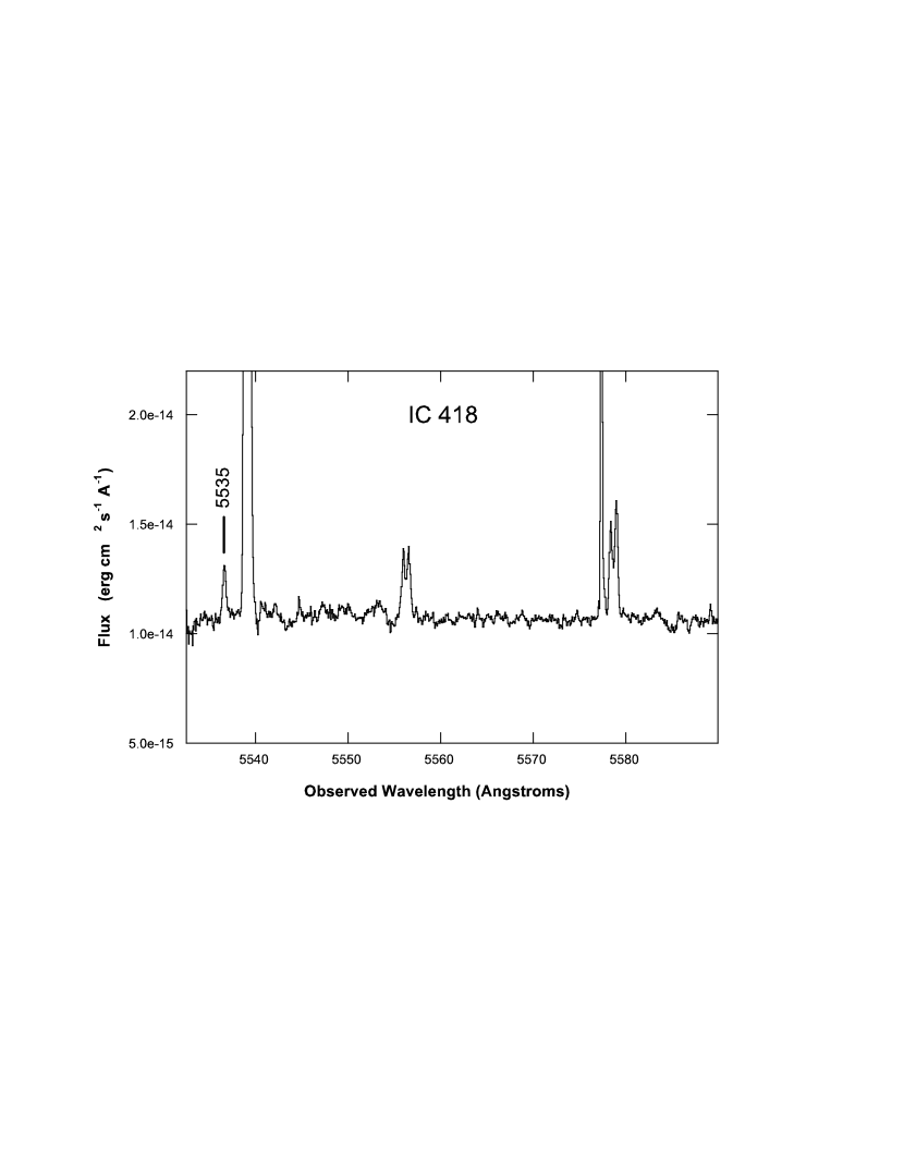
Figure 1: A portion of our echelle spectrum of IC 418, showing the emission line at 5535Å that is used as an example in Table 2.

As an illustration of EMILI output and results, we consider the identification of an emission line observed at 5536.60Å in the spectrum of IC 418, with the relevant EMILI output for this line listed in Table 2. The data were obtained with the CTIO 4m echelle in Dec 2001 at a resolution of 9 km s${}^{-1}\,$(R=33,000), and the relevant wavelength region of that spectrum is shown in Fig. 1. The measured wavelength of the line is 5536.60Å, which when corrected for the +68.6 km s${}^{-1}\,$radial velocity of the object determined from the higher Balmer and Paschen lines, corresponds to a rest wavelength of 5535.33Å. Its observed flux relative to H$\beta$ is $4.5\times 10^{-5}$, and the line has a signal-to-noise ratio of S/N = 26 and a width (FWHM) of 17 km s${}^{-1}\,$. These measured line attributes appear in the first row of Table 2, and below this row in Columns A-K appear all lines listed in the v2.04 Atomic Line List that have wavelengths within 5$\sigma$ (about 20 km s${}^{-1}\,$or 0.37Å) of the observed line and which have template fluxes within a factor of $10^{3}$ of the brightest computed template flux for the entire group of candidate lines.

Column A lists the observed wavelength (air) of the unidentified lines corrected for any velocity shifts appropriate for the emitting ion of each candidate ID, according to the kinematical model. Transitions whose wavelengths are denoted by a “+” sign are within $1.5\sigma$ wavelength error from the measured line wavelength. The laboratory wavelength (in air) is given in Column B, and the emitting ion is listed in column C. Columns D and E give the predicted template flux for each candidate line and the difference between its wavelength and that of the measured line in units of velocity (km s${}^{-1}\,$). Column F lists the number of associated multiplet lines that should be observable compared to the number observed. In column G the Identification Index is given for each candidate line, and the capital alphabet letter following the numerical IDI gives the ranking of the line, with A representing the most likely ID, i.e., the lowest IDI value. Finally, in columns H/I/J/K appear the wavelengths of the strongest associated multiplet lines that are possibly observed together with their differences in wavelength (in km s${}^{-1}\,$) from those of the observed lines. Our experience shows that when the associated lines are truly that, and not just coincidences, their differences in wavelength from the observed lines are virtually identical to the difference between the primary line and its measured line wavelength.

Looking in detail at the EMILI results for the observed IC 418 λ5536.60Å line, a secure identification with N II $\lambda$5535.35Å is indicated, although an ID with C II $\lambda$5535.35Å is also a possibility. The N II line has a slightly (insignificantly) better wavelength agreement with the observed line than the C II transition, although the C II line is predicted to be slightly brighter than the N II line using the generic cross sections and abundances. Both putative ID’s have computed template fluxes that are higher than that of the observed line. The key to the identification devolves to the associated multiplet lines for the two transitions: both possible lines in the N II multiplet are apparently present whereas the one possible associated line for the C II line is not observed. The former lines could conceivably be due to chance coincidences with unrelated transitions, however the wavelength differences between the N II associated line wavelengths and those of the observed lines are very similar: -1.0 km s${}^{-1}\,$for the primary line vs. –2.9 and –1.3 km s${}^{-1}\,$for its associated multiplet lines, which argues against chance coincidences. The lack of detection of the C II associated multiplet line could be due to a number of factors having nothing to do with its true intensity, including its location at the very edge of an echelle order or its superposition on a strong night sky line or scattered ghost feature. Consequently, its non-detection may be explainable. These doubts can be addressed by visual inspection of both the original 2-dimensional spectral image and the final reduced 1-dimensional spectrum. This final manual check of the EMILI results is an important component of proper line identification when there are several competing transitions that are credible ID’s.

It is worth noting that the particular N II $\lambda$5535.35Å transition discussed above is a quartet line whose upper level is an autoionizing state that lies above the N⁺ ionizing continuum. It is therefore almost certainly excited by dielectronic recombination of N⁺². Of particular significance is the fact that all three possible stabilizing transitions from the autoionizing state are observed in IC 418, making their identification quite secure.

We have applied EMILI to the full, final reduced high S/N echelle spectrum of IC 418 obtained at CTIO. We employed an updated version of the v2.04 Atomic Line List that includes higher level lines of He I, and a standard set of parameters in computing template fluxes for putative line ID’s, i.e., solar abundances, and $n_{e}=10^{4}$ cm^-3 and $T_{e}=10^{4}$ K. In making final ID’s for this nebula we have used the EMILI results as the initial basis for considering final line assignments, however we have not blindly accepted the EMILI recommendation for each line. Rather, we have studied the entire spectrum and have considered the entire list of ID’s collectively, using our judgment as to what lines we believe constitute the most reasonable identifications, and these are presented for the entire spectrum in Table 3.

In most cases we have accepted the EMILI top-ranked ID as the final ID. However, for some lines we have selected one of the ID’s whose IDI was not the smallest of the candidate group, as evidenced by the ranking given in column (6) of Table 3. For almost every line our final ID was one that was ranked by EMILI as one of the four most probable lines, and we have listed all the final identifications together with the observed lines and their measured wavelengths and reddening corrected fluxes in the Table. When the lowest value of IDI for an assigned line is higher than IDI$\geq$5 we consider the ID to be uncertain and therefore tag that ID with a colon. When the most likely putative ID has IDI$\geq$8 we place a “?” after the ID, believing that the ID does not have a solid basis and that the spectral feature may be spurious or the line list does not contain the correct transition for that feature. This line list should constitute one of the most detailed emission spectra of any PNe, and can serve as an archetype of low ionization spectra, similar to the spectrum of the Orion Nebula presented by Baldwin et al. (2000).

EMILI found solid identifications for 620 of the 807 observed IC 418 emission lines, and possible identifications for an additional 72 lines. Table 3 notes for each line those identifications that are not rated as questionable. There are a total of 750 such line identifications, for 476 observed lines for which there was only one suggested identification and for a further 144 observed lines for which there is more than one possible identification. The dereddened strengths of these identified lines range down to slightly below $10^{-5}$ the intensity of H$\beta$.

5 Comparision Of EMILI Results With Previous Studies

The correctness of spectral line identifications, especially for fainter lines that are not frequently observed, is difficult to ascertain. There is no absolute benchmark of correct ID’s with which to compare the results of EMILI, except possibly for the stronger lines in spectra which have been observed in many objects and for which there is universal agreement. We will therefore undertake to compare EMILI results with those of previous studies done traditionally as an indication of their reliability.

We are currently engaged in a program to obtain high S/N spectra of a sample of emission-line objects to which we can apply EMILI. At present we have excellent data for IC 418 (Sharpee, Baldwin, & Williams, 2003), and we have access to high resolution spectra of the Orion Nebula (Baldwin et al., 2000), for which detailed traditional line identifications have also been made. For IC 418 we compare the EMILI identifications from this study with those made by Hyung, Aller, & Feibelman (1994) from their Lick Observatory echelle data.

We have taken the spectra of IC 418 and the Orion Nebula, and have generated the necessary line characterization and wavelength error tables from rdgen. This information has been fed into EMILI using our updated v2.04 version of the line database and standard nebular parameters with solar abundances. Line identifications have been made, and when the lowest value of the IDI has been shared by more than one line all of those lines are assigned as ID’s. The resulting identifications have then been compared with the published ID’s for the Orion Nebula and IC 418. The comparison of EMILI ID’s with those assigned traditionally for these nebulae is given in Table 4. The EMILI ID rankings A, B, C, & D refer to the first, second, third, and fourth highest ranked ID’s from the algorithm. The comparison shows that the EMILI identifications ranked as “A” agree with the traditional manual ID for about 85% of all lines. Furthermore, 90–98 % of all manual ID’s are ranked as A, B, C, or D by EMILI. The agreement with those ranked A can be improved upon easily by optimizing the way in the ID Index is defined. We have taken a close look at some of the disagreements between the manual ID’s and those ranked ‘A’ by EMILI, and we believe that EMILI is more likely to be correct than the traditional line identifications in a majority of cases. This raises the question as to which identification process, traditional or software, yields more correct results. This question can only be answered after a larger sample of objects have been studied at fainter flux levels so that some consensus emerges as to the correct identification of the weakest lines.

6 Summary and Future Prospects

The time- and labor-intensive method of traditional identification of spectral lines has acted as a deterrent to obtaining very high S/N, high resolution spectra of astronomical objects. The task of making manual identifications for large numbers of lines has required such effort that the focus has been on utilizing only well-known stronger lines as diagnostics to determine physical conditions. Yet, modern spectrographs and detectors make very faint lines observable with only a modest investment of telescope time, and the large amount of new information that is certain to be contained in previously unstudied weak lines can now be tapped.

Even with its current simple logic EMILI works well in identifying lines in nebular spectra, and certainly well enough to justify continued improvement. It would benefit from new features such as the ability to interrogate multiple line databases, and using additional criteria to evaluate candidate ID’s, including a more sophisticated way to deconvolve line blends. Also, it should be applied to the spectra of additional types of emission-line objects. One of the eventual goals is to include very heavy elements in the line lists so that s- and r-process elements can be identified when lines from these elements are detected in spectra. This may require detecting lines down to $10^{-6}$ the intensity of H$\beta$. This flux level is 100 times fainter than the nebular continuum of the emitting gas upon which the lines are superposed, however the requisite S/N is achievable. The very large numbers of emission lines that would be revealed in such spectra are precisely the situation that requires an automated line identification aid such as EMILI.

The logic incorporated into EMILI is based upon traditional procedures used by spectroscopists for making manual line identifications in astronomical spectra. There are a number of uncertainties involved in the application of EMILI to spectra, and a number of areas in which improvements should eventually be made. One of the major difficulties of spectral line identification is accurately characterizing blends of multiple lines. It is often difficult to prove whether a feature is or is not a blend, and what the component wavelengths and line widths are when it is a blend. Emission-line objects can have a complex kinematical structure that results in complicated line profiles which differ from ion to ion of the same element. For example, a line of sight that passes through an expanding shell, as is the case for the object IC 418, produces a distinct double-peaked profile that is easily misinterpreted as two separate lines rather than a single feature. The stronger signature lines in the spectrum easily remove this uncertainty because they generally do not suffer significant blending and can therefore be used to characterize the different line profiles. For the current version of EMILI only a cursory effort was made to use differing intrinsic line widths and profiles as identification discriminants because of the complexity involved in doing proper line deconvolutions for large numbers of lines. However, these criteria should be developed further in future versions of EMILI.

One of the most important aspects of faint line detection is the use of spectral resolution that can resolve the narrowest lines in the spectrum, which is set by the thermal widths of the lines (typically, of order 10 km s${}^{-1}\,$) and bulk motions in the gas. Higher spectral resolution increases the accuracy of measured line wavelengths, which is the most important criterion in making line ID’s, and it serves to increase the contrast between peak line intensity and the surrounding continuum. The detectability of emission lines is further enhanced by low bulk velocities of the gas and by the faintest possible continuum against which the lines are detected. One cannot escape the bound-free and 2-photon continuum emitted by the ionized gas, but one can select objects of low dust content in order to minimize the contribution of the scattered continuum from the ionizing star. The number density of lines increases at fainter intensity levels and the proper identification of the weakest lines becomes increasingly uncertain due to the less well determined wavelengths of these features and the higher fraction of associated multiplet lines that are not observed because their S/N is below the threshold of detection. This is inevitable, and there will always be a substantial fraction of lines at the threshold of detection for which the criteria for confirmation are not well determined. Line ID’s for the faintest lines are generally less certain, and further progress can be made by pressing for spectra with yet higher S/N, since the faintest flux levels we have achieved do not approach a line density that is so high that weak lines blend into each other to form a pseudo-continuum.

Finally, the v2.04 Atomic Line List is the only database that we have interrogated in searching for potential identifications in the present version of EMILI, and its wavelengths are accepted as valid for each transition. A more thorough search process should eventually interrogate multiple line lists and should include molecular lines, especially those that are known to be present in the night sky spectrum (Osterbrock et al., 1996). Imperfect sky subtraction inevitably results in night sky lines being present in the spectra of many objects, and even though these lines are not intrinsic to the object they do require proper identification.

The current line identification software is still in a rudimentary form, yet it is already shown to be reliable and efficient in making an arduous process consistent and tractable. EMILI produces the largest gains over the traditional method in situations where there are large numbers of lines to be identified, as in our deep echelle spectra of IC418. For spectra of lower resolution the current version of EMILI is likely to be less successful because of the importance that it assigns to wavelength accuracy. We are experimenting with making the relative weights given to the identification criteria variable and dependent upon the resolution and S/N of the spectrum. Further refinement of the software logic and steady progress in compiling more complete transition databases should produce a reliable product, and have a dramatic impact on high S/N spectroscopy in the next decade.

.

Table 1: Signature Lines for Ionization Bins.

Bin	Energy Range (eV)	Signature Lines
A	0-13.6	Mg I] $\lambda 4571$, Na I $\lambda 5890,5896,$
		[S I] $\lambda 7775$, [C I] $\lambda 8727$
		Ca II (H&K) $\lambda 3934,3968$
B	13.6-24.7	H$\beta$
C	24.7-54.5	He I $\lambda 5876,4471$
D	54.5-100.0	He II $\lambda 4686$
E	$>100$	[Fe X] $\lambda 6375$, [Ne V] $\lambda 3426$,
		[Fe VII] $\lambda 6087$, [Ar X] $\lambda 5533$

Table 2: Sample EMILI Output.

Observed Line: 5536.60 Flux: 4.5E-05 S/N: 26.40 FWHM: 16.9
A	B	C		D	E	F	G	H	I	J	K
5535.36	5535.040	P	IV	1.3E-06	17.4	2/0	*
5535.33	5535.169	Mn	II	9.4E-06	8.6	5/1	9	5764.280	8.7
+ 5535.36	5535.325	Ni	III	5.4E-06	1.9	5/0	7D
+ 5535.33	5535.347	N	II	3.1E-04	-1.0	2/2	1A	5530.242	-2.9	5551.922	-1.3
+ 5535.33	5535.353	C	II	1.1E-03	-1.4	1/0	3B
+ 5535.33	5535.383	Fe	II]	1.6E-06	-3.0	7/0	7D
+ 5535.33	5535.384	N	II	3.1E-04	-3.1	8/1	4C	5526.234	-3.1
5535.28	5535.378	[V	II]	8.2E-05	-5.1	7/0	7D
5535.36	5535.476	Fe	III	9.9E-05	-6.2	8/0	8
5535.28	5535.413	Fe	I]	2.5E-06	-7.0	5/0	9
5535.28	5535.418	Fe	I	5.6E-05	-7.3	5/0	8
5535.33	5535.466$	Ar	II	1.0E-05	-7.5	0/0	7D
5535.28	5535.455	Mg	I	3.5E-05	-9.3	0/0	7D
5535.33	5535.525$	S	II	4.9E-05	-10.7	0/0	7D

Table 3: EMILI Line Indentifications for IC 418

$\lambda_{o}$	FWHM	$F(\lambda)/F(\textrm{H}\beta)$	$I(\lambda)/I(\textrm{H}\beta)$	S/N	IDI	ID	$\lambda$	$\delta$V	Lower Term/Config	Upper Term/Config	$J_{l}$	$J_{u}$	Multi
(Å)	(km/s)	($F(\textrm{H}\beta)=100$)	($I(\textrm{H}\beta)=100$)				(Å)	(km/s)
(1)	(2)	(3)	(4)	(5)	(6)	(7)	(8)	(9)	(10)	(11)	(12)	(13)	(14)
3512.511	22.9	0.1026	0.1365	37.6	2 A	He I	3512.505	-0.5	3Po 1s.2p	3D 1s.12d	2.0	****	0/0
3530.499	24.6	0.1509	0.2002	99990.0	3 A	He I	3530.482	-1.5	3Po 1s.2p	3D 1s.11d	2.0	****	1/0
3554.417	23.1	0.1771	0.2340	127.5	3 A	He I	3554.389	-2.4	3Po 1s.2p	3D 1s.10d	1.0	****	2/0
3560.616	20.3	0.0049	0.0065	7.3	$\cdots$	$\cdots$	$\cdots$	$\cdots$	$\cdots$	$\cdots$	$\cdots$	$\cdots$	$\cdots$
3562.932	20.7	0.0138	0.0182	11.5	4 A	He I	3562.969	3.1	3Po 1s.2p	3S 1s.10s	2.0	1.0	1/0
3574.775	13.5	0.0036	0.0047	7.2	6 B	O II	3574.845 :	5.9	2D 2s2.2p2.(3P).3d	2Po 2s2.2p2.(3P).5p	1.5	1.5	2/0
					8 D	N II	3574.900 ?	10.5	3P 2s.2p2.(4P).3d	3Do 2s.2p2.(4P).5p	2.0	2.0	2/0
3579.402	23.4	0.0103	0.0135	8.1	$\cdots$	$\cdots$	$\cdots$	$\cdots$	$\cdots$	$\cdots$	$\cdots$	$\cdots$	$\cdots$
3587.284	24.4	0.2549	0.3351	161.6	3 A	He I	3587.253	-2.6	3Po 1s.2p	3D 1s.9d	2.0	****	1/0
3590.815	25.3	0.0192	0.0252	21.9	5 A	C II	3590.757	-4.8	4D 2s.2p.(3Po).3p	4Po 2s.2p.(3Po).4s	1.5	0.5	7/0
					7 C	C II	3590.876 :	5.1	4D 2s.2p.(3Po).3p	4Po 2s.2p.(3Po).4s	2.5	1.5	5/0
3601.327	14.8	0.0021	0.0027	7.2	$\cdots$	$\cdots$	$\cdots$	$\cdots$	$\cdots$	$\cdots$	$\cdots$	$\cdots$	$\cdots$
3606.862	24.6	0.0053	0.0070	7.3	$\cdots$	$\cdots$	$\cdots$	$\cdots$	$\cdots$	$\cdots$	$\cdots$	$\cdots$	$\cdots$
3613.634	21.7	0.4259	0.5577	293.5	2 A	He I	3613.642	0.6	1S 1s.2s	1Po 1s.5p	0.0	1.0	0/0
3616.798	20.7	0.0045	0.0059	11.0	3 A	S II	3616.767	-2.6	2Do 3s2.3p2.(3P).4p	2P 3s2.3p2.(3P).4d	2.5	1.5	1/0
3634.250	25.7	0.3883	0.5069	156.7	4 A	He I	3634.231	-1.6	3Po 1s.2p	3D 1s.8d	2.0	3.0	2/0
3649.872	32.6	0.0109	0.0141	7.5	$\cdots$	$\cdots$	$\cdots$	$\cdots$	$\cdots$	$\cdots$	$\cdots$	$\cdots$	$\cdots$
3652.003	24.0	0.0254	0.0331	25.9	3 A	He I	3651.981	-1.8	3Po 1s.2p	3S 1s.8s	2.0	1.0	1/0
3654.256	9.3	0.0052	0.0067	7.7	$\cdots$	H I	3654.266	0.8	2 2*	42 42*	****	****	$\cdots$
3654.681	14.3	0.0107	0.0140	10.2	2 A	N II	3654.670 ?	-0.9	3F 2s.2p2.(4P).3d	3Do 2s.2p2.(2D).3p	4.0	3.0	2/1
					$\cdots$	H I	3654.676	-0.4	2 2*	41 41*	****	****	$\cdots$
3655.113	11.1	0.0114	0.0148	13.5	2 A	H I	3655.117	0.3	2 2*	40 40*	****	****	0/0
					$\cdots$	N II	3655.050 ?	-5.2	3F 2s.2p2.(4P).3d	3Do 2s.2p2.(2D).3p	3.0	2.0	$\cdots$
3655.588	11.6	0.0135	0.0176	19.0	2 A	H I	3655.593	0.4	2 2*	39 39*	****	****	0/0
					$\cdots$	N II	3655.500 ?	-7.2	3F 2s.2p2.(4P).3d	3Do 2s.2p2.(2D).3p	1.0	1.0	$\cdots$
3656.104	12.5	0.0231	0.0300	32.5	3 A	H I	3656.106	0.2	2 2*	38 38*	****	****	0/0
3656.667	13.5	0.0270	0.0352	44.9	2 A	H I	3656.663	-0.3	2 2*	37 37*	****	****	0/0
3657.276	16.2	0.0451	0.0586	54.9	2 A	H I	3657.267	-0.7	2 2*	36 36*	****	****	0/0
3657.936	18.1	0.0758	0.0986	96.0	2 A	H I	3657.923	-1.1	2 2*	35 35*	****	****	0/0
3658.647	19.9	0.0932	0.1212	102.1	2 A	H I	3658.639	-0.7	2 2*	34 34*	****	****	0/0
3659.428	23.5	0.1402	0.1823	126.5	2 A	H I	3659.421	-0.6	2 2*	33 33*	****	****	0/0
3660.286	26.3	0.1871	0.2433	152.8	2 A	H I	3660.277	-0.7	2 2*	32 32*	****	****	0/0
3661.230	27.9	0.2274	0.2956	193.0	2 A	H I	3661.218	-1.0	2 2*	31 31*	****	****	0/0
3662.262	29.1	0.2669	0.3470	266.4	2 A	H I	3662.256	-0.5	2 2*	30 30*	****	****	0/0
3663.406	30.7	0.3058	0.3975	267.6	2 A	H I	3663.404	-0.2	2 2*	29 29*	****	****	0/0
3664.683	31.3	0.3548	0.4610	353.9	2 A	H I	3664.676	-0.6	2 2*	28 28*	****	****	0/0
3666.098	31.4	0.3970	0.5158	364.1	2 A	H I	3666.095	-0.2	2 2*	27 27*	****	****	0/0
3669.463	31.4	0.5017	0.6514	456.3	3 A	H I	3669.464	0.1	2 2*	25 25*	****	****	0/0
3671.475	31.4	0.5339	0.6930	557.6	2 A	H I	3671.475	0.0	2 2*	24 24*	****	****	0/0
3673.757	32.3	0.5922	0.7684	565.0	2 A	H I	3673.758	0.1	2 2*	23 23*	****	****	0/0
3676.361	32.8	0.6586	0.8542	486.9	3 A	H I	3676.362	0.1	2 2*	22 22*	****	****	0/0
3679.349	33.2	0.7847	1.0173	464.0	3 A	H I	3679.352	0.2	2 2*	21 21*	****	****	0/0
3682.806	34.3	0.8182	1.0602	256.7	2 A	H I	3682.808	0.2	2 2*	20 20*	****	****	0/0
3686.830	32.5	0.9390	1.2159	307.2	3 A	H I	3686.830	0.0	2 2*	19 19*	****	****	0/0
3691.556	32.6	1.1469	1.4841	289.2	2 A	H I	3691.554	-0.2	2 2*	18 18*	****	****	0/0
3697.156	33.5	1.2877	1.6649	436.3	2 A	H I	3697.152	-0.3	2 2*	17 17*	****	****	0/0
3703.852	31.8	1.4822	1.9143	455.8	3 A	H I	3703.852	0.0	2 2*	16 16*	****	****	0/0
3705.017	22.8	0.5795	0.7483	224.3	4 A	He I	3704.996	-1.7	3Po 1s.2p	3D 1s.7d	2.0	3.0	2/0
3711.968	32.0	1.7773	2.2926	726.1	3 A	H I	3711.971	0.2	2 2*	15 15*	****	****	0/0
3721.895	36.3	2.5687	3.3082	439.6	6 B	[S III]	3721.630 :	-21.4	3P 3s2.3p2	1S 3s2.3p2	1.0	0.0	0/0
					5 A	H I	3721.938 :	3.5	2 2*	14 14*	****	****	0/0
3726.035	41.9	96.1832	123.7908	8543.0	0 A	[O II]	3726.032	-0.2	4So 2s2.2p3	2Do 2s2.2p3	1.5	1.5	1/1
3728.785	43.2	40.6870	52.3426	4280.0	1 A	[O II]	3728.815	2.4	4So 2s2.2p3	2Do 2s2.2p3	1.5	2.5	1/1
3734.364	31.0	2.3876	3.0689	614.9	3 A	H I	3734.368	0.3	2 2*	13 13*	****	****	0/0
3735.506	38.9	0.0461	0.0593	35.1	8 C	O II	3735.722 ?	17.3	2Po 2s2.2p2.(1D).3p	2D 2s2.2p2.(1D).4s	1.5	1.5	2/0
					0$<$	O II	3735.786 ?	22.5	2Po 2s2.2p2.(1D).3p	2D 2s2.2p2.(1D).4s	1.5	2.5	2/0
3750.149	31.6	3.1656	4.0585	1262.0	3 A	H I	3750.151	0.2	2 2*	12 12*	****	****	0/0
3756.065	37.4	0.0610	0.0782	37.2	4 A	He I	3756.115	4.0	1Po 1s.2p	1D 1s.14d	1.0	2.0	0/0
3768.782	23.2	0.0238	0.0304	38.3	3 A	He I	3768.821	3.1	1Po 1s.2p	1D 1s.13d	1.0	2.0	0/0
3770.631	31.8	3.8028	4.8591	1284.0	3 A	H I	3770.630	-0.1	2 2*	11 11*	****	****	0/0
					7 B	He I	3770.750 :	9.5	1Po 1s.2p	1S 1s.13s	1.0	0.0	0/0
3777.164	41.5	0.0039	0.0050	9.4	5 A	Ne II	3777.134 :	-2.4	4P 2s2.2p4.(3P).3s	4Po 2s2.2p4.(3P).3p	0.5	1.5	6/0
3780.171	33.1	0.0035	0.0045	8.6	$\cdots$	$\cdots$	$\cdots$	$\cdots$	$\cdots$	$\cdots$	$\cdots$	$\cdots$	$\cdots$
3784.851	22.5	0.0294	0.0374	71.6	3 A	He I	3784.895	3.5	1Po 1s.2p	1D 1s.12d	1.0	2.0	0/0
					9 B	O II	3784.990 ?	11.0	2Po 2s2.2p2.(3P).4p	2D 2s2.2p2.(1D).4d	1.5	2.5	2/0
3795.635	30.0	0.0019	0.0025	6.6	$\cdots$	$\cdots$	$\cdots$	$\cdots$	$\cdots$	$\cdots$	$\cdots$	$\cdots$	$\cdots$
3797.897	31.5	4.4534	5.6643	1187.0	2 A	H I	3797.898	0.1	2 2*	10 10*	****	****	0/0
3801.360	55.5	0.0055	0.0070	10.7	$\cdots$	$\cdots$	$\cdots$	$\cdots$	$\cdots$	$\cdots$	$\cdots$	$\cdots$	$\cdots$
3802.720	37.6	0.0057	0.0073	11.9	8	S II	3802.604 ?	-9.1	4Po 3s2.3p2.(3P).4p	4P 3s2.3p2.(3P).4d	1.5	0.5	6/0
3805.736	20.3	0.0331	0.0421	99.5	3 A	He I	3805.777	3.2	1Po 1s.2p	1D 1s.11d	1.0	2.0	0/0
3811.854	9.0	0.0015	0.0019	9.9	6 C	S II	3811.745 :	-8.6	2Po 3s2.3p2.(3P).4p	2D 3s2.3p2.(3P).4d	0.5	1.5	2/0
3813.451	26.5	0.0026	0.0033	7.6	$\cdots$	$\cdots$	$\cdots$	$\cdots$	$\cdots$	$\cdots$	$\cdots$	$\cdots$	$\cdots$
3817.159	25.2	0.0027	0.0035	7.7	$\cdots$	$\cdots$	$\cdots$	$\cdots$	$\cdots$	$\cdots$	$\cdots$	$\cdots$	$\cdots$
3819.628	23.9	0.8853	1.1218	525.4	4 A	He I	3819.603	-2.0	3Po 1s.2p	3D 1s.6d	2.0	2.0	4/0
3821.849	26.8	0.0038	0.0049	18.3	$\cdots$	$\cdots$	$\cdots$	$\cdots$	$\cdots$	$\cdots$	$\cdots$	$\cdots$	$\cdots$
3829.745	21.3	0.0184	0.0232	34.2	3 A	N II	3829.795	3.9	3P 2s2.2p.(2Po).3p	3Po 2s2.2p.(2Po).4s	1.0	2.0	4/2
3831.645	20.6	0.0237	0.0300	58.1	9	S II	3831.379 ?	-20.8	2Po 3s2.3p2.(3P).4p	2D 3s2.3p2.(3P).4d	1.5	2.5	2/0
					7 C	C II	3831.726 :	6.3	2Po 2s2.4p	2D 2s.2p.(3Po).3p	1.5	2.5	2/0
3833.550	20.0	0.0539	0.0681	105.7	3 A	He I	3833.584	2.7	1Po 1s.2p	1D 1s.10d	1.0	2.0	0/0
3834.140	25.2	0.0024	0.0030	8.3	$\cdots$	$\cdots$	$\cdots$	$\cdots$	$\cdots$	$\cdots$	$\cdots$	$\cdots$	$\cdots$
3835.387	32.0	7.5117	9.4921	2711.0	2 A	H I	3835.384	-0.2	2 2*	9 9*	****	****	0/0
3838.349	25.5	0.0581	0.0734	98.5	7 D	S III	3838.268 :	-6.3	3Po 3s2.3p.4s	3P 3s2.3p.4p	2.0	2.0	3/1
					5 A	N II	3838.374 :	1.9	3P 2s2.2p.(2Po).3p	3Po 2s2.2p.(2Po).4s	2.0	2.0	3/1
3842.183	19.1	0.0100	0.0126	33.6	2 A	N II	3842.187	0.3	3P 2s2.2p.(2Po).3p	3Po 2s2.2p.(2Po).4s	0.0	1.0	5/3
3848.265	35.0	0.0217	0.0274	56.4	3 A	Mg II	3848.212	-4.1	2D 3d	2Po 5p	2.5	1.5	2/1
					7	Mg II	3848.341 :	5.9	2D 3d	2Po 5p	1.5	1.5	2/0
3850.392	45.2	0.0183	0.0231	46.1	2 A	Mg II	3850.386	-0.5	2D 3d	2Po 5p	1.5	0.5	2/1
3853.755	36.3	0.0046	0.0058	11.2	5 A	Si II	3853.664	-7.1	2D 3s.3p2	2Po 3s2.(1S).4p	1.5	1.5	2/0
3855.089	29.6	0.0078	0.0098	29.9	2 A	N II	3855.096	0.5	3P 2s2.2p.(2Po).3p	3Po 2s2.2p.(2Po).4s	1.0	0.0	5/3
3856.054	45.6	0.0805	0.1013	188.1	1 A	Si II	3856.018	-2.8	2D 3s.3p2	2Po 3s2.(1S).4p	2.5	1.5	2/2
					2 B	N II	3856.063	0.7	3P 2s2.2p.(2Po).3p	3Po 2s2.2p.(2Po).4s	2.0	1.0	4/3
					6 C	O II	3856.134 :	6.2	4Do 2s2.2p2.(3P).3p	4D 2s2.2p2.(3P).3d	1.5	0.5	9/1
3862.619	40.6	0.0337	0.0424	110.2	1 A	Si II	3862.596	-1.8	2D 3s.3p2	2Po 3s2.(1S).4p	1.5	0.5	2/2
3867.486	21.7	0.0677	0.0851	183.6	3 A	He I	3867.472	-1.1	3Po 1s.2p	3S 1s.6s	2.0	1.0	1/0
3868.745	13.6	2.4614	3.0916	805.3	0$<$	[Ne III]	3869.060	24.4	3P 2s2.2p4	1D 2s2.2p4	2.0	2.0	1/1
3871.781	21.2	0.0606	0.0760	183.0	3 A	He I	3871.830	3.8	1Po 1s.2p	1D 1s.9d	1.0	2.0	0/0
3873.477	15.2	0.0014	0.0018	8.6	7	Fe I	3873.594 ?	9.0	z5Po 3d6.(5D).4s.4p.(3Po)	5D 3d6.4s.(6D).6s	3.0	3.0	4/1
3876.477	43.7	0.0055	0.0069	12.1	5 D	C II	3876.392	-6.6	4Fo 2s.2p.(3Po).3d	4G 2s.2p.(3Po).4f	3.5	4.5	5/0
					8	C II	3876.653	13.6	4Fo 2s.2p.(3Po).3d	4G 2s.2p.(3Po).4f	2.5	3.5	8/0
					8	C II	3876.186	-22.5	4Fo 2s.2p.(3Po).3d	4G 2s.2p.(3Po).4f	4.5	5.5	2/0
3882.178	13.7	0.0050	0.0063	27.4	3 A	O II	3882.194	1.2	4Do 2s2.2p2.(3P).3p	4D 2s2.2p2.(3P).3d	3.5	3.5	3/1
					0$<$	O II	3882.446	-20.7	4Do 2s2.2p2.(3P).3p	4D 2s2.2p2.(3P).3d	1.5	1.5	7/0
3883.110	23.7	0.0022	0.0027	10.3	4 A	O II	3883.137	2.1	4Do 2s2.2p2.(3P).3p	4D 2s2.2p2.(3P).3d	3.5	2.5	4/1
3884.008	16.9	0.0011	0.0014	8.8	6 A	C II	3883.853 :	-12.0	4Fo 2s.2p.(3Po).3d	4G 2s.2p.(3Po).4f	4.5	3.5	5/1
3888.939	66.4	12.8101	16.0294	3433.0	5 A	H I	3889.049	8.5	2 2*	8 8*	****	****	0/0
					0$<$	He I	3888.605	-25.8	3S 1s.2s	3Po 1s.3p	****	****	$\cdots$
3891.462	25.5	0.0027	0.0034	99990.0	6 A	Ar II :	3891.401 ?	-4.7	4D 3s2.3p4.(3P).3d	4Do 3s2.3p4.(3P).4p	0.5	0.5	9/1
3892.335	14.0	0.0021	0.0027	8.0	5 B	S II :	3892.288	-3.6	4Po 3s2.3p2.(3P).4p	4P 3s2.3p2.(3P).4d	2.5	2.5	3/0
3892.769	31.0	0.0020	0.0025	13.4	$\cdots$	$\cdots$	$\cdots$	$\cdots$	$\cdots$	$\cdots$	$\cdots$	$\cdots$	$\cdots$
3895.096	32.9	0.0032	0.0040	7.4	8	Fe I	3895.232 ?	10.5	z5Po 3d6.(5D).4s.4p.(3Po)	5D 3d6.4s.(6D).6s	2.0	2.0	7/1
3896.201	27.7	0.0044	0.0055	13.7	6 A	O II :	3896.303 :	7.9	4Do 2s2.2p2.(3P).3p	4P 2s2.2p2.(3P).3d	2.5	1.5	5/0
					6 A	Fe I	3896.349 :	11.4	z5Po 3d6.(5D).4s.4p.(3Po)	5D 3d6.4s.(6D).6s	1.0	0.0	8/2
3899.208	44.9	0.0064	0.0080	15.8	7	S III	3899.028 :	-13.8	3Po 3s2.3p.4s	3P 3s2.3p.4p	2.0	1.0	4/0
3907.470	21.9	0.0028	0.0035	13.5	3 A	O II	3907.455	-1.2	4Do 2s2.2p2.(3P).3p	4P 2s2.2p2.(3P).3d	2.5	2.5	4/0
3909.251	9.6	0.0015	0.0019	7.6	$\cdots$	$\cdots$	$\cdots$	$\cdots$	$\cdots$	$\cdots$	$\cdots$	$\cdots$	$\cdots$
3918.930	18.7	0.0858	0.1068	226.4	4 A	C II	3918.967	2.8	2Po 2s2.3p	2S 2s2.4s	0.5	0.5	1/1
3920.640	18.3	0.1650	0.2052	372.8	3 A	C II	3920.682	3.2	2Po 2s2.3p	2S 2s2.4s	1.5	0.5	1/1
3923.200	36.9	0.0035	0.0043	14.6	$\cdots$	$\cdots$	$\cdots$	$\cdots$	$\cdots$	$\cdots$	$\cdots$	$\cdots$	$\cdots$
3924.007	36.9	0.0029	0.0036	7.9	$\cdots$	$\cdots$	$\cdots$	$\cdots$	$\cdots$	$\cdots$	$\cdots$	$\cdots$	$\cdots$
3926.544	21.8	0.1013	0.1258	247.6	3 A	He I	3926.544	0.0	1Po 1s.2p	1D 1s.8d	1.0	2.0	0/0
					3 A	O II	3926.581	2.8	4Do 2s2.2p2.(3P).3p	4P 2s2.2p2.(3P).3d	3.5	2.5	2/2
3929.127	18.5	0.0023	0.0028	5.8	5 A	C II	3928.970 :	-12.0	2Fo 2s2.4f	2G 2s2.14g	****	****	$\cdots$
3935.956	22.3	0.0119	0.0147	43.8	1 A	He I	3935.945	-0.8	1Po 1s.2p	1S 1s.8s	1.0	0.0	0/0
3962.513	44.8	0.0048	0.0059	9.6	$\cdots$	$\cdots$	$\cdots$	$\cdots$	$\cdots$	$\cdots$	$\cdots$	$\cdots$	$\cdots$
3963.797	17.1	0.0012	0.0014	7.7	$\cdots$	$\cdots$	$\cdots$	$\cdots$	$\cdots$	$\cdots$	$\cdots$	$\cdots$	$\cdots$
3964.727	22.1	0.8384	1.0336	509.9	2 A	He I	3964.729	0.1	1S 1s.2s	1Po 1s.4p	0.0	1.0	0/0
3967.457	14.2	0.7914	0.9751	229.6	0$<$	[Ne III]	3967.790	25.2	3P 2s2.2p4	1D 2s2.2p4	1.0	2.0	1/1
3970.074	31.9	13.6820	16.8492	2775.0	3 A	H I	3970.072	-0.1	2 2*	7 7*	****	****	0/0
3977.342	25.5	0.0021	0.0026	9.6	6 A	C II	3977.250 :	-6.9	4Do 2s.2p.(3Po).3d	4D 2s.2p.(3Po).4f	2.5	2.5	6/0
3979.851	24.8	0.0016	0.0020	10.7	$\cdots$	S II	3979.824	-2.0	4So 3s2.3p2.(3P).4p	4P 3s2.3p2.(3P).4d	1.5	0.5	$\cdots$
3986.459	30.2	0.0027	0.0034	9.7	$\cdots$	$\cdots$	$\cdots$	$\cdots$	$\cdots$	$\cdots$	$\cdots$	$\cdots$	$\cdots$
3988.516	25.8	0.0039	0.0048	9.9	$\cdots$	$\cdots$	$\cdots$	$\cdots$	$\cdots$	$\cdots$	$\cdots$	$\cdots$	$\cdots$
3992.088	33.4	0.0007	0.0008	7.0	$\cdots$	Ar II	3992.088 ?	0.0	4D 3s2.3p4.(3P).3d	4Do 3s2.3p4.(3P).4p	1.5	2.5	$\cdots$
3998.781	32.7	0.0073	0.0089	19.9	8	N III	3998.630 ?	-11.3	2D 2s2.4d	2Fo 2s2.5f	1.5	2.5	2/0
					1 A	S II	3998.759	-1.6	4So 3s2.3p2.(3P).4p	4P 3s2.3p2.(3P).4d	1.5	1.5	2/2
4004.939	33.7	0.0026	0.0032	8.2	7	Ni III	4005.180 ?	18.0	3F 3d7.(4F).4d	3Do 3d6.(5D).4s.4p	4.0	3.0	2/1
4009.256	21.7	0.1522	0.1860	367.9	1 A	He I	4009.256	0.0	1Po 1s.2p	1D 1s.7d	1.0	2.0	0/0
4015.931	20.1	0.0034	0.0041	15.3	$\cdots$	$\cdots$	$\cdots$	$\cdots$	$\cdots$	$\cdots$	$\cdots$	$\cdots$	$\cdots$
4018.473	25.1	0.0009	0.0012	9.4	7 D	Ni III	4018.760 ?	21.4	3F 3d7.(4F).4d	3Do 3d6.(5D).4s.4p	3.0	2.0	5/2
4023.993	18.8	0.0176	0.0215	79.7	7 C	O II	4023.868 :	-9.3	2F 2s2.2p2.(1D).3d	2[2]o 2s2.2p2.(1D).4f.D	3.5	2.5	$\cdots$
					1 A	He I	4023.980	-1.0	1Po 1s.2p	1S 1s.7s	1.0	0.0	0/0
4026.207	22.9	1.7237	2.0978	412.4	8	N II	4026.078 ?	-9.6	3Fo 2s2.2p.(2Po).3d	2[9/2] 2s2.2p.(2Po$<$3/2$>$).4f.G	3.0	4.0	$\cdots$
					4 B	He I	4026.186	-1.6	3Po 1s.2p	3D 1s.5d	2.0	2.0	4/0
4027.209	31.7	0.0280	0.0340	99999.0	3 A	Fe I	4027.098 ?	-8.3	y5Fo 3d7.(4F).4p	g5G 3d6.4s.(4D).4d	5.0	4.0	5/2
4028.221	12.6	0.0045	0.0055	12.2	$\cdots$	$\cdots$	$\cdots$	$\cdots$	$\cdots$	$\cdots$	$\cdots$	$\cdots$	$\cdots$
4032.779	51.5	0.0080	0.0098	12.6	3 A	S II	4032.767	-0.9	4So 3s2.3p2.(3P).4p	4P 3s2.3p2.(3P).4d	1.5	2.5	1/1
4035.165	37.9	0.0059	0.0071	16.6	3 A	N II	4035.081	-6.2	3Fo 2s2.2p.(2Po).3d	2[7/2] 2s2.2p.(2Po$<$3/2$>$).4f.G	2.0	3.0	$\cdots$
					4 B	O II	4035.073	-6.8	4F 2s2.2p2.(3P).3d	2[3]o 2s2.2p2.(3P).4f.F	2.5	2.5	$\cdots$
4041.303	24.9	0.0100	0.0121	30.2	2 A	O II	4041.278	-1.9	4F 2s2.2p2.(3P).3d	2[2]o 2s2.2p2.(3P).4f.F	2.5	2.5	$\cdots$
					3 B	N II	4041.310	0.5	3Fo 2s2.2p.(2Po).3d	2[9/2] 2s2.2p.(2Po$<$3/2$>$).4f.G	4.0	5.0	$\cdots$
4043.460	24.3	0.0033	0.0041	8.7	4 A	N II	4043.532	5.3	3Fo 2s2.2p.(2Po).3d	2[7/2] 2s2.2p.(2Po$<$3/2$>$).4f.G	3.0	4.0	$\cdots$
4058.287	16.8	0.0035	0.0043	10.3	4 A	N II	4058.162	-9.2	3Fo 2s2.2p.(2Po).3d	2[7/2] 2s2.2p.(2Po$<$3/2$>$).4f.G	4.0	3.0	$\cdots$
4065.230	25.5	0.0045	0.0055	23.4	4 A	Fe III	4065.253 ?	1.7	5Ho 3d5.(4G).5p	5G 3d5.(4G).6s	4.0	5.0	8/1
4067.329	22.2	0.0030	0.0036	6.2	$\cdots$	$\cdots$	$\cdots$	$\cdots$	$\cdots$	$\cdots$	$\cdots$	$\cdots$	$\cdots$
4068.668	48.8	1.4822	1.7873	900.8	0 A	[S II]	4068.600	-5.0	4So 3s2.3p3	2Po 3s2.3p3	1.5	1.5	1/1
4069.626	18.9	0.0169	0.0204	99999.0	1 A	O II	4069.623	-0.2	4Do 2s2.2p2.(3P).3p	4F 2s2.2p2.(3P).3d	0.5	1.5	8/6
4069.888	13.0	0.0165	0.0199	99999.0	1 A	O II	4069.882	-0.4	4Do 2s2.2p2.(3P).3p	4F 2s2.2p2.(3P).3d	1.5	2.5	8/6
4072.149	15.2	0.0272	0.0327	100.3	1 A	O II	4072.153	0.3	4Do 2s2.2p2.(3P).3p	4F 2s2.2p2.(3P).3d	2.5	3.5	5/4
4074.505	35.9	0.0085	0.0102	19.2	5 B	N III	4074.460 :	-3.3	4P 2p2.(3P).3d	4Po 2s.2p.(3Po).8d	1.5	****	2/0
					3 A	C II	4074.481	-1.8	4Do 2s.2p.(3Po).3d	4F 2s.2p.(3Po).4f	0.5	1.5	8/1
					5 B	C II	4074.544 :	2.9	4Do 2s.2p.(3Po).3d	4F 2s.2p.(3Po).4f	1.5	2.5	8/0
4075.889	17.0	0.0368	0.0442	99999.0	2 A	O II	4075.862	-2.0	4Do 2s2.2p2.(3P).3p	4F 2s2.2p2.(3P).3d	3.5	4.5	2/2
					5 C	C II	4075.940 :	3.8	4Do 2s.2p.(3Po).3d	4F 2s.2p.(3Po).4f	2.5	2.5	7/1
4076.374	46.7	0.6358	0.7653	352.0	1 A	[S II]	4076.349	-1.8	4So 3s2.3p3	2Po 3s2.3p3	1.5	0.5	1/1
4078.808	16.3	0.0047	0.0056	23.0	2 A	O II	4078.842	2.5	4Do 2s2.2p2.(3P).3p	4F 2s2.2p2.(3P).3d	1.5	1.5	8/5
4079.643	36.0	0.0021	0.0025	10.6	4 A	[Fe III]	4079.700	4.2	5D 3d6	3G 3d6	3.0	4.0	7/1
4082.319	36.0	0.0044	0.0053	13.3	9	Fe I	4082.107 ?	-15.6	z5Fo 3d6.(5D).4s.4p.(3Po)	g5D 3d6.4s.(4D).5s	2.0	2.0	*/1
					4 A	N II	4082.271	-3.5	3Fo 2s2.2p.(2Po).3d	2[7/2] 2s2.2p.(2Po$<$1/2$>$).4f.F	3.0	4.0	$\cdots$
4083.874	14.3	0.0040	0.0049	17.9	3 A	[Fe II]	4083.781	-6.8	a4F 3d7	b2H 3d6.(3H).4s	4.5	4.5	3/0
					3 A	O II	4083.899	1.8	4F 2s2.2p2.(3P).3d	2[4]o 2s2.2p2.(3P).4f.G	2.5	3.5	$\cdots$
4084.670	20.5	0.0039	0.0047	22.5	*	Fe I	4084.492 ?	-13.1	z5Fo 3d6.(5D).4s.4p.(3Po)	g5D 3d6.4s.(4D).5s	5.0	4.0	2/0
4085.101	16.7	0.0064	0.0076	22.5	1 A	O II	4085.112	0.8	4Do 2s2.2p2.(3P).3p	4F 2s2.2p2.(3P).3d	2.5	2.5	7/5
4087.146	14.5	0.0037	0.0045	24.5	2 A	O II	4087.153	0.5	4F 2s2.2p2.(3P).3d	2[3]o 2s2.2p2.(3P).4f.G	1.5	2.5	$\cdots$
4089.290	13.3	0.0095	0.0114	37.9	2 A	O II	4089.288	-0.2	4F 2s2.2p2.(3P).3d	2[5]o 2s2.2p2.(3P).4f.G	4.5	5.5	$\cdots$
4092.920	10.8	0.0027	0.0032	16.8	1 A	O II	4092.929	0.6	4Do 2s2.2p2.(3P).3p	4F 2s2.2p2.(3P).3d	3.5	3.5	4/3
4093.921	39.5	0.0041	0.0049	11.0	6 C	Fe III	4093.645 :	-20.2	5Go 3d5.(4G).5p	5G 3d5.(4G).5d	3.0	2.0	*/4
					5 A	N III	4093.680 :	-17.7	2Do 2s.2p.(1Po).3d	2D 2s.2p.(3Po).6p	1.5	1.5	3/2
4095.648	19.4	0.0035	0.0042	10.5	7	N III	4095.340 :	-22.6	2Do 2s.2p.(1Po).3d	2D 2s.2p.(3Po).6p	2.5	1.5	3/1
					2 A	O II	4095.644	-0.3	4F 2s2.2p2.(3P).3d	2[3]o 2s2.2p2.(3P).4f.G	2.5	3.5	$\cdots$
4096.513	11.8	0.0024	0.0028	15.6	5 A	[Fe III]	4096.610 :	7.1	5D 3d6	3G 3d6	2.0	3.0	8/1
4097.265	14.9	0.0096	0.0115	42.8	2 A	O II	4097.225	-2.9	4Po 2s2.2p2.(3P).3p	4D 2s2.2p2.(3P).3d	0.5	1.5	7/4
					2 A	O II	4097.257	-0.6	4F 2s2.2p2.(3P).3d	2[4]o 2s2.2p2.(3P).4f.G	3.5	4.5	$\cdots$
4101.739	31.5	20.7242	24.8041	5729.0	2 A	H I	4101.734	-0.4	2 2*	6 6*	****	****	0/0
4104.747	55.1	0.0134	0.0160	18.1	1 A	O II	4104.724	-1.7	4Po 2s2.2p2.(3P).3p	4D 2s2.2p2.(3P).3d	1.5	2.5	5/4
4104.996	14.2	0.0038	0.0046	10.4	1 A	O II	4104.990	-0.4	4Po 2s2.2p2.(3P).3p	4D 2s2.2p2.(3P).3d	1.5	1.5	7/3
4108.454	33.4	0.0046	0.0055	7.8	$\cdots$	$\cdots$	$\cdots$	$\cdots$	$\cdots$	$\cdots$	$\cdots$	$\cdots$	$\cdots$
4110.766	15.0	0.0063	0.0075	19.2	1 A	O II	4110.786	1.5	4Po 2s2.2p2.(3P).3p	4D 2s2.2p2.(3P).3d	1.5	0.5	7/4
4113.028	53.6	0.0068	0.0082	16.2	5 B	Fe I	4112.912 ?	-8.5	y5Do 3d7.(4F).4p	i5D 3d6.4s.(4D).4d	3.0	3.0	6/1
4119.214	17.3	0.0184	0.0219	61.2	1 A	O II	4119.216	0.2	4Po 2s2.2p2.(3P).3p	4D 2s2.2p2.(3P).3d	2.5	3.5	2/2
4120.312	17.4	0.0057	0.0068	99999.0	2 A	O II	4120.278	-2.5	4Po 2s2.2p2.(3P).3p	4D 2s2.2p2.(3P).3d	2.5	2.5	4/3
					0$<$	O II	4120.547	17.1	4Po 2s2.2p2.(3P).3p	4D 2s2.2p2.(3P).3d	2.5	1.5	5/1
4120.829	22.8	0.1730	0.2062	351.8	3 A	He I	4120.811	-1.4	3Po 1s.2p	3S 1s.5s	2.0	1.0	1/0
4121.434	17.5	0.0140	0.0166	99999.0	2 A	O II	4121.462	2.1	4Po 2s2.2p2.(3P).3p	4P 2s2.2p2.(3P).3d	0.5	0.5	6/2
4123.658	15.5	0.0016	0.0019	7.8	$\cdots$	$\cdots$	$\cdots$	$\cdots$	$\cdots$	$\cdots$	$\cdots$	$\cdots$	$\cdots$
4128.569	18.6	0.0136	0.0162	7.1	7 C	Fe II	4128.748 :	13.0	b4P 3d6.(3P4).4s	z4Do 3d6.(5D).4p	2.5	1.5	5/0
4131.757	19.8	0.0311	0.0370	92.4	8 B	Fe II	4131.870 ?	8.2	z4Ho 3d6.(3H).4p	e4G 3d6.(5D).4d	4.5	4.5	7/1
4132.789	11.5	0.0070	0.0083	34.8	3 A	O II	4132.800	0.8	4Po 2s2.2p2.(3P).3p	4P 2s2.2p2.(3P).3d	0.5	1.5	6/1
4139.999	32.8	0.0024	0.0028	11.2	$\cdots$	$\cdots$	$\cdots$	$\cdots$	$\cdots$	$\cdots$	$\cdots$	$\cdots$	$\cdots$
4143.758	23.1	0.2649	0.3140	226.1	4 B	O II	4143.739	-1.4	6P 2s.2p3.(5So).3p	6Do 2s.2p3.(5So).3d	2.5	3.5	5/1
					1 A	He I	4143.759	0.1	1Po 1s.2p	1D 1s.6d	1.0	2.0	0/0
4146.047	19.9	0.0050	0.0059	17.3	3 A	Ne II	4146.064	1.2	2P 2s2.2p4.(3P).4s	2So 2s2.2p4.(3P).5p	0.5	0.5	1/0
					4 B	O II	4146.076	2.1	6P 2s.2p3.(5So).3p	6Do 2s.2p3.(5So).3d	3.5	4.5	2/0
4153.287	15.1	0.0156	0.0184	75.7	3 A	O II	4153.298	0.8	4Po 2s2.2p2.(3P).3p	4P 2s2.2p2.(3P).3d	1.5	2.5	4/1
4156.328	30.3	0.0134	0.0159	48.5	4 A	N II	4156.358	2.1	3Do 2s2.2p.(2Po).3d	2[3/2] 2s2.2p.(2Po$<$3/2$>$).4f.D	1.0	2.0	$\cdots$
					7 D	O II	4156.530 :	14.6	4Po 2s2.2p2.(3P).3p	4P 2s2.2p2.(3P).3d	2.5	1.5	4/1
4161.141	29.6	0.0018	0.0022	9.5	$\cdots$	$\cdots$	$\cdots$	$\cdots$	$\cdots$	$\cdots$	$\cdots$	$\cdots$	$\cdots$
4167.285	31.6	0.0032	0.0038	10.9	$\cdots$	$\cdots$	$\cdots$	$\cdots$	$\cdots$	$\cdots$	$\cdots$	$\cdots$	$\cdots$
4168.995	24.3	0.0393	0.0463	140.0	1 A	He I	4168.972	-1.7	1Po 1s.2p	1S 1s.6s	1.0	0.0	0/0
					8 C	O II	4169.224 :	16.4	4Po 2s2.2p2.(3P).3p	4P 2s2.2p2.(3P).3d	2.5	2.5	3/1
4176.145	27.3	0.0054	0.0064	13.0	3 A	N II	4176.159	1.0	1Do 2s2.2p.(2Po).3d	2[5/2] 2s2.2p.(2Po$<$1/2$>$).4f.F	2.0	3.0	$\cdots$
4185.433	16.2	0.0069	0.0081	22.9	1 A	O II	4185.439	0.4	2Fo 2s2.2p2.(1D).3p	2G 2s2.2p2.(1D).3d	2.5	3.5	2/1
4187.368	33.6	0.0029	0.0034	7.4	8	Fe II	4187.493 ?	9.0	z4Ho 3d6.(3H).4p	e4G 3d6.(5D).4d	4.5	5.5	5/0
4188.379	11.5	0.0010	0.0011	8.2	$\cdots$	$\cdots$	$\cdots$	$\cdots$	$\cdots$	$\cdots$	$\cdots$	$\cdots$	$\cdots$
4189.783	21.2	0.0106	0.0124	34.0	2 A	O II	4189.788	0.3	2Fo 2s2.2p2.(1D).3p	2G 2s2.2p2.(1D).3d	3.5	4.5	2/1
					8	O II	4189.581 ?	-14.5	2Fo 2s2.2p2.(1D).3p	2G 2s2.2p2.(1D).3d	3.5	3.5	2/0
4192.167	48.9	0.0021	0.0024	9.8	8	O II	4192.512 ?	24.7	2Do 2s2.2p2.(1D).3p	2P 2s2.2p2.(1D).3d	2.5	1.5	2/0
4196.805	36.1	0.0048	0.0056	13.5	7 D	O II	4196.698 :	-7.6	2Do 2s2.2p2.(1D).3p	2P 2s2.2p2.(1D).3d	1.5	0.5	2/0
4208.038	30.3	0.0053	0.0061	20.1	$\cdots$	$\cdots$	$\cdots$	$\cdots$	$\cdots$	$\cdots$	$\cdots$	$\cdots$	$\cdots$
4211.316	24.5	0.0069	0.0081	32.8	7 C	[Fe II]	4211.099 :	-15.5	a4F 3d7	b2H 3d6.(3H).4s	3.5	5.5	4/0
4219.753	19.9	0.0013	0.0015	8.0	2 A	Ne II	4219.745	-0.6	4D 2s2.2p4.(3P).3d	2[4]o 2s2.2p4.(3P$<$2$>$).4f	3.5	4.5	$\cdots$
					7	Ni III	4220.070 ?	22.5	3F 3d7.(4F).4d	3Do 3d6.(5D).4s.4p	2.0	3.0	4/2
4236.926	14.3	0.0026	0.0030	18.0	2 A	N II	4236.927	0.1	3Do 2s2.2p.(2Po).3d	2[5/2] 2s2.2p.(2Po$<$1/2$>$).4f.F	1.0	2.0	$\cdots$
					6	N II	4237.047 :	8.6	3Do 2s2.2p.(2Po).3d	2[7/2] 2s2.2p.(2Po$<$1/2$>$).4f.F	2.0	3.0	$\cdots$
4241.809	19.9	0.0060	0.0069	30.2	4 B	N II	4241.756	-3.8	3Do 2s2.2p.(2Po).3d	2[5/2] 2s2.2p.(2Po$<$1/2$>$).4f.F	2.0	3.0	$\cdots$
					3 A	N II	4241.786	-1.6	3Do 2s2.2p.(2Po).3d	2[7/2] 2s2.2p.(2Po$<$1/2$>$).4f.F	3.0	4.0	$\cdots$
4246.861	25.6	0.0027	0.0031	9.2	5 B	N II	4246.706 :	-10.9	3Do 2s2.2p.(2Po).3d	2[5/2] 2s2.2p.(2Po$<$1/2$>$).4f.F	3.0	2.0	$\cdots$
4253.919	38.7	0.0064	0.0074	15.8	2 A	O II	4253.894	-1.8	2G 2s2.2p2.(1D).3d	2[5]o 2s2.2p2.(1D).4f.H	4.5	5.5	$\cdots$
					2 A	O II	4253.907	-0.8	2G 2s2.2p2.(1D).3d	2[5]o 2s2.2p2.(1D).4f.H	4.5	4.5	$\cdots$
4256.128	23.5	0.0037	0.0043	13.5	$\cdots$	$\cdots$	$\cdots$	$\cdots$	$\cdots$	$\cdots$	$\cdots$	$\cdots$	$\cdots$
4259.506	19.4	0.0040	0.0046	15.9	$\cdots$	$\cdots$	$\cdots$	$\cdots$	$\cdots$	$\cdots$	$\cdots$	$\cdots$	$\cdots$
4267.161	38.7	0.4963	0.5712	536.0	8 D	C II	4267.001	-11.3	2D 2s2.3d	2Fo 2s2.4f	1.5	2.5	2/0
					5 A	C II	4267.183	1.5	2D 2s2.3d	2Fo 2s2.4f	2.5	3.5	2/0
					8 D	C II	4267.261	7.0	2D 2s2.3d	2Fo 2s2.4f	2.5	2.5	2/0
4271.882	44.2	0.0050	0.0058	7.1	5 C	Fe I	4271.760 ?	-8.5	a3F 3d7.(4F).4s	z3Go 3d7.(4F).4p	4.0	5.0	2/0
4275.535	13.5	0.0056	0.0065	33.4	5 B	Fe II]	4275.492 ?	-3.0	z2Po 3d6.(3P4).4p	4P 3d6.(5D).4d	0.5	0.5	4/1
					2 A	O II	4275.551	1.1	4D 2s2.2p2.(3P).3d	2[4]o 2s2.2p2.(3P).4f.F	3.5	4.5	$\cdots$
4276.820	44.0	0.0068	0.0079	23.5	6 B	O II	4276.749 :	-5.0	4D 2s2.2p2.(3P).3d	2[3]o 2s2.2p2.(3P).4f.F	2.5	3.5	$\cdots$
					4 A	[Fe II]	4276.829	0.7	a4F 3d7	a4G 3d6.(3G).4s	3.5	4.5	5/1
4277.481	24.9	0.0029	0.0033	10.7	3 A	O II	4277.426	-3.9	4D 2s2.2p2.(3P).3d	2[3]o 2s2.2p2.(3P).4f.F	3.5	2.5	$\cdots$
					3 A	O II	4277.427	-3.8	4D 2s2.2p2.(3P).3d	2[2]o 2s2.2p2.(3P).4f.F	0.5	1.5	$\cdots$
4280.548	48.9	0.0022	0.0026	7.4	4 B	Fe II]	4280.542 ?	-0.4	z2Po 3d6.(3P4).4p	4P 3d6.(5D).4d	1.5	0.5	4/1
4281.246	20.9	0.0016	0.0019	9.1	3 B	O II	4281.313	4.7	4P 2s2.2p2.(3P).3d	2[2]o 2s2.2p2.(3P).4f.D	2.5	2.5	$\cdots$
4282.957	16.1	0.0022	0.0026	13.4	2 A	O II	4282.961	0.3	4D 2s2.2p2.(3P).3d	2[2]o 2s2.2p2.(3P).4f.F	1.5	2.5	$\cdots$
4285.699	13.2	0.0027	0.0031	16.5	2 A	O II	4285.684	-1.1	2F 2s2.2p2.(3P).3d	2[3]o 2s2.2p2.(3P).4f.F	2.5	3.5	$\cdots$
					5 C	Fe II	4285.716 ?	1.2	x4Do 3d6.(3F4).4p	e4F 3d6.(5D).4d	2.5	2.5	7/1
4287.234	12.1	0.0048	0.0055	99999.0	7 B	[Fe II]	4287.394 :	11.2	a6D 3d6.(5D).4s	a6S 3d5.4s2	4.5	2.5	1/0
4287.551	15.1	0.0072	0.0083	99999.0	5 A	[Co II]	4287.499 ?	-3.6	a3F 3d8	b3P 3d7.(4P).4s	3.0	1.0	5/1
					7 C	O II	4287.727 :	12.3	2Po 2s2.2p2.(1D).3p	2D 2s2.2p2.(3P).4d	1.5	1.5	2/1
4292.406	21.2	0.0078	0.0089	35.2	6 B	O II :	4292.214 ?	-13.4	2F 2s2.2p2.(3P).3d	2[2]o 2s2.2p2.(3P).4f.F	2.5	2.5	$\cdots$
					6 B	C II	4292.250 :	-10.9	2Fo 2s2.2p.(3Po).3d	2G 2s2.10g	****	****	$\cdots$
4294.777	27.8	0.0051	0.0059	21.1	2 A	O II	4294.782	0.3	4P 2s2.2p2.(3P).3d	2[2]o 2s2.2p2.(3P).4f.D	1.5	2.5	$\cdots$
					6 B	O II	4294.919 :	9.9	4P 2s2.2p2.(3P).3d	2[2]o 2s2.2p2.(3P).4f.D	1.5	1.5	$\cdots$
4300.454	27.4	0.0030	0.0034	7.8	$\cdots$	$\cdots$	$\cdots$	$\cdots$	$\cdots$	$\cdots$	$\cdots$	$\cdots$	$\cdots$
4303.129	16.9	0.0009	0.0010	7.9	4 A	O II	4303.072	-4.0	2G 2s2.2p2.(1D).3d	2[4]o 2s2.2p2.(1D).4f.G	3.5	****	$\cdots$
4303.819	14.6	0.0058	0.0066	34.1	2 A	O II	4303.823	0.3	4P 2s2.2p2.(3P).3d	2[3]o 2s2.2p2.(3P).4f.D	2.5	3.5	$\cdots$
4306.069	20.1	0.0061	0.0069	20.2	7 A	[Fe II]	4305.890 :	-12.5	a4F 3d7	a4G 3d6.(3G).4s	2.5	2.5	8/0
					7 A	O II	4305.965 :	-7.2	2D 2s2.2p2.(1D).3d	2[1]o 2s2.2p2.(1D).4f.P	1.5	****	$\cdots$
4307.269	19.5	0.0105	0.0119	45.3	3 A	O II	4307.232	-2.6	4P 2s2.2p2.(3P).3d	2[2]o 2s2.2p2.(3P).4f.D	0.5	1.5	$\cdots$
4317.119	16.4	0.0140	0.0159	57.8	1 A	O II	4317.139	1.4	4P 2s2.2p2.(3P).3s	4Po 2s2.2p2.(3P).3p	0.5	1.5	6/5
					8	C II	4317.265 ?	10.1	4P 2s.2p.(3Po).3p	4Po 2s.2p.(3Po).4s	2.5	2.5	3/0
4318.581	25.2	0.0076	0.0086	32.5	5 A	C II	4318.606 :	1.7	4P 2s.2p.(3Po).3p	4Po 2s.2p.(3Po).4s	0.5	1.5	6/1
4319.618	13.8	0.0073	0.0083	38.4	2 A	O II	4319.629	0.8	4P 2s2.2p2.(3P).3s	4Po 2s2.2p2.(3P).3p	1.5	2.5	4/4
					4 B	[Fe II]	4319.620 ?	0.1	a4F 3d7	a4G 3d6.(3G).4s	2.5	3.5	8/1
					8 C	Fe II	4319.680 ?	4.3	x4Do 3d6.(3F4).4p	e4F 3d6.(5D).4d	2.5	3.5	5/1
4321.597	48.3	0.0070	0.0080	11.5	5 A	C II	4321.657	4.2	4P 2s.2p.(3Po).3p	4Po 2s.2p.(3Po).4s	1.5	1.5	6/1
4323.326	70.0	0.0082	0.0093	8.2	3 B	[Co II]	4323.278 ?	-3.4	a3F 3d8	b3P 3d7.(4P).4s	3.0	2.0	4/1
					8	C II	4323.106 ?	-15.3	4P 2s.2p.(3Po).3p	4Po 2s.2p.(3Po).4s	0.5	0.5	6/0
4325.866	45.0	0.0151	0.0171	49.4	8	O II	4325.761 ?	-7.3	4P 2s2.2p2.(3P).3s	4Po 2s2.2p2.(3P).3p	0.5	0.5	6/0
					4 A	Fe I	4325.762 ?	-7.2	a3F 3d7.(4F).4s	z3Go 3d7.(4F).4p	2.0	3.0	5/1
					4 A	C II	4325.833 ?	-2.3	4P 2s.2p.(3Po).3p	4Po 2s.2p.(3Po).4s	2.5	1.5	4/0
4329.876	21.4	0.0062	0.0070	20.7	6 B	C II	4329.675 :	-13.9	2D 2s2.4d	2Fo 2s2.9f	****	****	$\cdots$
4335.866	60.2	0.0082	0.0093	8.7	$\cdots$	$\cdots$	$\cdots$	$\cdots$	$\cdots$	$\cdots$	$\cdots$	$\cdots$	$\cdots$
4336.830	11.5	0.0033	0.0037	12.2	1 A	O II	4336.859	2.0	4P 2s2.2p2.(3P).3s	4Po 2s2.2p2.(3P).3p	1.5	1.5	6/5
4340.465	31.6	39.6376	44.8053	6397.0	3 A	H I	4340.464	-0.1	2 2*	5 5*	****	****	0/0
4345.546	15.8	0.0170	0.0192	39.6	1 A	O II	4345.560	1.0	4P 2s2.2p2.(3P).3s	4Po 2s2.2p2.(3P).3p	1.5	0.5	6/5
4347.990	26.0	0.0046	0.0052	9.3	$\cdots$	O II	4347.413 ?	-39.9	2D 2p2.(1D).3s	2Do 2s2.2p2.(1D).3p	1.5	1.5	$\cdots$
					$\cdots$	O II	4347.217 ?	-53.3	2D 2p2.(1D).3s	2Do 2s2.2p2.(1D).3p	2.5	1.5	$\cdots$
4349.409	18.6	0.0292	0.0330	77.3	0 A	O II	4349.426	1.2	4P 2s2.2p2.(3P).3s	4Po 2s2.2p2.(3P).3p	2.5	2.5	3/3
4351.266	19.2	0.0071	0.0080	16.5	5 A	O II	4351.260 :	-0.4	2D 2s2.2p2.(1D).3s	2Do 2s2.2p2.(1D).3p	2.5	2.5	3/0
					9 C	O II	4351.457 ?	13.2	2D 2s2.2p2.(1D).3s	2Do 2s2.2p2.(1D).3p	1.5	2.5	3/0
4359.380	42.0	0.0080	0.0090	27.9	3 A	[Fe II]	4359.333	-3.2	a6D 3d6.(5D).4s	a6S 3d5.4s2	3.5	2.5	2/0
					5 B	O II	4359.395 :	1.0	2Do 2s2.2p2.(3P).3p	2D 2s2.2p2.(3P).3d	1.5	2.5	3/0
4363.191	15.6	0.8321	0.9353	606.3	1 A	[O III]	4363.210	1.3	1D 2s2.2p2	1S 2s2.2p2	2.0	0.0	0/0
4366.875	13.4	0.0121	0.0136	53.0	1 A	O II	4366.895	1.3	4P 2s2.2p2.(3P).3s	4Po 2s2.2p2.(3P).3p	2.5	1.5	4/4
4368.264	54.9	0.0858	0.0964	291.3	2 A	O I	4368.193	-4.9	3So 2s2.2p3.(4So).3s	3P 2s2.2p3.(4So).4p	****	****	$\cdots$
4376.580	12.6	0.0014	0.0016	11.0	4 A	C II	4376.582	0.1	4Po 2s.2p.(3Po).3d	4D 2s.2p.(3Po).4f	1.5	2.5	5/0
4387.930	21.5	0.4889	0.5462	291.0	1 A	He I	4387.929	-0.1	1Po 1s.2p	1D 1s.5d	1.0	2.0	0/0
4390.550	47.1	0.0053	0.0059	32.0	$\cdots$	$\cdots$	$\cdots$	$\cdots$	$\cdots$	$\cdots$	$\cdots$	$\cdots$	$\cdots$
4391.963	15.8	0.0020	0.0022	7.4	3 A	Ne II	4391.991	1.9	4F 2s2.2p4.(3P).3d	2[5]o 2s2.2p4.(3P$<$2$>$).4f	4.5	5.5	$\cdots$
					3 A	Ne II	4391.995	2.2	4F 2s2.2p4.(3P).3d	2[5]o 2s2.2p4.(3P$<$2$>$).4f	4.5	4.5	$\cdots$
4393.483	33.9	0.0041	0.0045	15.0	4 A	O II	4393.435	-3.3	2Po 2s2.2p2.(1D).3p	2P 2s2.2p2.(3P).4d	1.5	0.5	3/0
4396.586	20.4	0.0014	0.0016	7.7	4 A	O I	4396.560 ?	-1.8	3P 2s2.2p3.(4So).4p	3Do 2s2.2p3.(2Do).4s	2.0	3.0	2/0
4411.172	13.3	0.0015	0.0016	12.5	4 A	C II	4411.152	-1.4	2Do 2s.2p.(3Po).3d	2F 2s.2p.(3Po).4f	1.5	2.5	2/0
4413.609	12.4	0.0025	0.0027	99999.0	$\cdots$	$\cdots$	$\cdots$	$\cdots$	$\cdots$	$\cdots$	$\cdots$	$\cdots$	$\cdots$
4413.942	10.4	0.0019	0.0021	99999.0	3 A	[Fe II]	4413.781	-10.9	a6D 3d6.(5D).4s	a6S 3d5.4s2	2.5	2.5	3/2
4414.888	15.0	0.0273	0.0303	113.7	1 A	O II	4414.898	0.7	2P 2s2.2p2.(3P).3s	2Do 2s2.2p2.(3P).3p	1.5	2.5	2/1
4416.090	11.0	0.0015	0.0016	99999.0	6 A	[Fe II]	4416.266 :	12.0	a6D 3d6.(5D).4s	b4F 3d6.(3F4).4s	4.5	4.5	3/1
4416.515	17.4	0.0024	0.0026	99999.0	7 B	[Fe II]	4416.266 :	-16.9	a6D 3d6.(5D).4s	b4F 3d6.(3F4).4s	4.5	4.5	3/0
4416.969	15.5	0.0178	0.0197	92.2	3 A	O II	4416.975	0.4	2P 2s2.2p2.(3P).3s	2Do 2s2.2p2.(3P).3p	0.5	1.5	2/1
4418.945	35.3	0.0029	0.0032	11.1	5 C	O II	4418.870 :	-5.1	2Po 2s2.2p2.(1S).3p	2P 2s2.2p2.(1D).4d	0.5	1.5	1/0
					3 A	Fe II	4418.958 ?	0.9	y4Go 3d6.(3F4).4p	e4F 3d6.(5D).4d	2.5	1.5	8/1
4432.692	22.1	0.0032	0.0036	11.4	6 B	[Fe II]	4432.447 :	-16.6	a6D 3d6.(5D).4s	b4F 3d6.(3F4).4s	3.5	2.5	7/1
					5 A	N II	4432.735 :	2.9	3Po 2s2.2p.(2Po).3d	2[5/2] 2s2.2p.(2Po$<$3/2$>$).4f.D	2.0	3.0	$\cdots$
4433.769	23.6	0.0025	0.0028	11.9	6	N II	4433.475 :	-19.9	3Po 2s2.2p.(2Po).3d	2[3/2] 2s2.2p.(2Po$<$3/2$>$).4f.D	0.0	1.0	$\cdots$
4437.552	22.0	0.0718	0.0792	211.5	1 A	He I	4437.554	0.1	1Po 1s.2p	1S 1s.5s	1.0	0.0	0/0
4447.060	16.5	0.0035	0.0039	19.7	2 A	N II	4447.030	-2.0	1P 2s2.2p.(2Po).3p	1Do 2s2.2p.(2Po).3d	1.0	2.0	0/0
4448.253	12.8	0.0008	0.0009	9.0	5 A	O II	4448.191 :	-4.2	2Fo 2s2.2p2.(1D).3p	2F 2s2.2p2.(1D).3d	3.5	3.5	3/0
4448.825	9.5	0.0009	0.0010	9.2	2 A	O II	4448.850	1.7	2P 2s2.2p2.(1D).3d	2[1]o 2s2.2p2.(1D).4f.P	1.5	****	$\cdots$
4452.262	43.9	0.0080	0.0088	34.1	4 A	[Fe II]	4452.098 ?	-11.1	a6D 3d6.(5D).4s	a6S 3d5.4s2	1.5	2.5	4/2
					8 C	O II	4452.378	7.8	2P 2s2.2p2.(3P).3s	2Do 2s2.2p2.(3P).3p	1.5	1.5	2/0
4453.475	16.3	0.0051	0.0056	29.1	7 D	Fe II	4453.205 ?	-18.2	y6Po 3d5.(6S).4s.4p.(3Po)	6P 3d6.(5D).4d	1.5	1.5	6/1
4454.107	21.5	0.0015	0.0017	6.5	8	O II	4453.966 ?	-9.5	4P 2s2.2p2.(3P).3d	4So 2s.2p3.(5So).3s	1.5	1.5	2/0
4457.091	20.9	0.0122	0.0134	59.4	3 A	Ne II	4457.050	-2.8	2D 2s2.2p4.(3P).3d	2[2]o 2s2.2p4.(3P$<$2$>$).4f	1.5	2.5	$\cdots$
					6 C	Ne II	4457.239 :	10.0	4P 2s2.2p4.(3P).3d	2[3]o 2s2.2p4.(3P$<$1$>$).4f	2.5	2.5	$\cdots$
					6 C	Ne II	4457.265 :	11.7	2D 2s2.2p4.(3P).3d	2[2]o 2s2.2p4.(3P$<$2$>$).4f	1.5	1.5	$\cdots$
4457.725	26.0	0.0026	0.0028	99999.0	6 A	[Fe II]	4457.945 :	14.8	a6D 3d6.(5D).4s	b4F 3d6.(3F4).4s	3.5	3.5	6/1
4459.898	17.2	0.0022	0.0025	14.3	6 A	N II	4459.937 :	2.6	3D 2s2.2p.(2Po).3p	3Po 2s2.2p.(2Po).3d	1.0	0.0	5/1
4465.404	14.8	0.0054	0.0059	32.4	1 A	O II	4465.408	0.3	6So 2s.2p3.(5So).3s	6P 2s.2p3.(5So).3p	2.5	3.5	1/1
					8	N II	4465.529 ?	8.4	3D 2s2.2p.(2Po).3p	3Po 2s2.2p.(2Po).3d	1.0	1.0	5/0
4466.390	25.1	0.0027	0.0029	9.9	3 A	O II	4466.435	3.0	2P 2s2.2p2.(3P).3d	2[2]o 2s2.2p2.(3P).4f.D	1.5	2.5	$\cdots$
					6 D	O II	4466.583 :	13.0	2P 2s2.2p2.(3P).3d	2[2]o 2s2.2p2.(3P).4f.D	1.5	1.5	$\cdots$
4467.919	14.7	0.0038	0.0041	22.6	1 A	O II	4467.924	0.3	6So 2s.2p3.(5So).3s	6P 2s.2p3.(5So).3p	2.5	2.5	2/2
					5 B	Fe II	4467.931 :	0.8	y4Go 3d6.(3F4).4p	e4F 3d6.(5D).4d	3.5	3.5	7/0
4469.375	13.5	0.0020	0.0022	12.1	1 A	O II	4469.378	0.2	6So 2s.2p3.(5So).3s	6P 2s.2p3.(5So).3p	2.5	1.5	2/2
					4 B	O II	4469.462	5.8	2P 2s2.2p2.(3P).3d	2[1]o 2s2.2p2.(3P).4f.D	0.5	0.5	$\cdots$
4471.499	23.7	4.1046	4.4921	1935.0	4 A	He I	4471.474	-1.7	3Po 1s.2p	3D 1s.4d	2.0	3.0	2/0
4474.689	20.9	0.0024	0.0026	5.8	4 A	[Fe II]	4474.904	14.4	a6D 3d6.(5D).4s	a6S 3d5.4s2	0.5	2.5	4/2
4477.745	25.1	0.0055	0.0061	29.9	4 A	N II	4477.682	-4.2	3D 2s2.2p.(2Po).3p	3Po 2s2.2p.(2Po).3d	2.0	1.0	5/1
4481.213	30.6	0.0176	0.0193	81.2	7 A	Mg II	4481.126 :	-5.8	2D 3d	2Fo 4f	2.5	3.5	2/0
					7 A	Mg II	4481.150 :	-4.2	2D 3d	2Fo 4f	2.5	2.5	2/0
					8 C	Mg II	4481.325 ?	7.5	2D 3d	2Fo 4f	1.5	2.5	2/0
4483.494	15.7	0.0018	0.0020	8.6	5 C	S II	4483.427 :	-4.5	4Do 3s2.3p2.(3P).4p	4P 3s2.3p2.(3P).5s	2.5	1.5	5/0
4485.231	34.2	0.0020	0.0021	10.5	7 B	Fe III	4485.575 :	23.0	3G 3d5.(2G3).4s	3Fo 3d5.(a2F).4p	5.0	4.0	2/1
4487.744	17.4	0.0008	0.0009	99999.0	7	Fe II	4487.497 :	-16.5	y6Po 3d5.(6S).4s.4p.(3Po)	6P 3d6.(5D).4d	2.5	2.5	6/1
					2 A	O II	4487.712	-2.2	2P 2s2.2p2.(1D).3d	2[2]o 2s2.2p2.(1D).4f.D	0.5	1.5	$\cdots$
4488.194	18.9	0.0022	0.0024	9.7	4 D	N II	4488.095	-6.6	3D 2s2.2p.(2Po).3p	3Po 2s2.2p.(2Po).3d	2.0	2.0	4/1
					2 A	O II	4488.184	-0.7	2P 2s2.2p2.(1D).3d	2[2]o 2s2.2p2.(1D).4f.D	1.5	2.5	$\cdots$
					2 A	O II	4488.198	0.3	2P 2s2.2p2.(1D).3d	2[2]o 2s2.2p2.(1D).4f.D	1.5	1.5	$\cdots$
					3 C	S II	4488.188	-0.4	2D 3s2.3p2.(3P).4d	2[2]o 3s2.3p2.(1D$<$2$>$).5f	1.5	****	$\cdots$
4489.468	23.0	0.0007	0.0007	7.0	3 A	O II	4489.461	-0.5	2P 2s2.2p2.(3P).3d	2[2]o 2s2.2p2.(3P).4f.D	0.5	1.5	$\cdots$
4491.278	19.6	0.0115	0.0125	56.5	5 B	C II	4491.130 :	-9.9	2Fo 2s2.4f	2G 2s2.9g	****	****	$\cdots$
					4 A	O II	4491.222	-3.7	2P 2s2.2p2.(3P).3d	2[3]o 2s2.2p2.(3P).4f.D	1.5	2.5	$\cdots$
4503.289	17.4	0.0014	0.0015	10.3	$\cdots$	$\cdots$	$\cdots$	$\cdots$	$\cdots$	$\cdots$	$\cdots$	$\cdots$	$\cdots$
4507.554	13.1	0.0047	0.0051	25.8	5 B	N II	4507.560 :	0.4	3D 2s2.2p.(2Po).3p	3Po 2s2.2p.(2Po).3d	3.0	2.0	2/0
4530.404	16.7	0.0039	0.0042	21.6	3 A	N II	4530.410	0.4	1Fo 2s2.2p.(2Po).3d	2[9/2] 2s2.2p.(2Po$<$3/2$>$).4f.G	3.0	4.0	$\cdots$
4545.218	23.6	0.0023	0.0024	11.8	$\cdots$	$\cdots$	$\cdots$	$\cdots$	$\cdots$	$\cdots$	$\cdots$	$\cdots$	$\cdots$
4552.505	22.1	0.0024	0.0026	11.3	3 A	N II	4552.522	1.1	1Fo 2s2.2p.(2Po).3d	2[7/2] 2s2.2p.(2Po$<$3/2$>$).4f.G	3.0	4.0	$\cdots$
4562.637	57.5	0.0387	0.0414	168.8	$\cdots$	$\cdots$	$\cdots$	$\cdots$	$\cdots$	$\cdots$	$\cdots$	$\cdots$	$\cdots$
4571.161	52.8	0.4017	0.4291	173.0	2 A	Mg I]	4571.096	-4.3	1S 3s2	3Po 3s.3p	0.0	1.0	0/0
4590.959	16.5	0.0135	0.0143	73.2	2 A	O II	4590.974	1.0	2D 2s2.2p2.(1D).3s	2Fo 2s2.2p2.(1D).3p	2.5	3.5	2/1
4596.171	15.5	0.0089	0.0094	37.8	8	O II	4595.957	-14.0	2D 2s2.2p2.(1D).3s	2Fo 2s2.2p2.(1D).3p	2.5	2.5	2/0
					2 A	O II	4596.176	0.3	2D 2s2.2p2.(1D).3s	2Fo 2s2.2p2.(1D).3p	1.5	2.5	2/1
4601.471	17.3	0.0248	0.0263	104.0	2 A	N II	4601.478	0.4	3Po 2s2.2p.(2Po).3s	3P 2s2.2p.(2Po).3p	1.0	2.0	4/4
4602.121	12.6	0.0020	0.0022	12.5	2 A	O II	4602.129	0.5	2D 2s2.2p2.(3P).3d	2[3]o 2s2.2p2.(3P).4f.F	1.5	2.5	$\cdots$
4607.140	17.5	0.0243	0.0257	96.0	4 A	[Fe III]	4607.030	-7.2	5D 3d6	3F4 3d6	4.0	3.0	4/1
					$\cdots$	N II	4607.153	0.8	3Po 2s2.2p.(2Po).3s	3P 2s2.2p.(2Po).3p	0.0	1.0	$\cdots$
4609.436	15.3	0.0057	0.0060	23.7	2 A	O II	4609.436	0.0	2D 2s2.2p2.(3P).3d	2[4]o 2s2.2p2.(3P).4f.F	2.5	3.5	$\cdots$
4611.738	41.4	0.0057	0.0061	8.1	5 B	O II	4611.582 :	-10.1	4F 2s2.2p2.(3P).4d	2[2]o 2s2.2p2.(1D).4f.D	2.5	2.5	$\cdots$
					5 B	O II	4611.597 :	-9.1	4F 2s2.2p2.(3P).4d	2[2]o 2s2.2p2.(1D).4f.D	2.5	1.5	$\cdots$
4613.858	19.6	0.0172	0.0182	59.1	6 D	O II	4613.681 :	-11.5	2D 2s2.2p2.(3P).3d	2[3]o 2s2.2p2.(3P).4f.F	2.5	3.5	$\cdots$
					2 A	N II	4613.868	0.7	3Po 2s2.2p.(2Po).3s	3P 2s2.2p.(2Po).3p	1.0	1.0	5/5
4620.348	21.5	0.0101	0.0107	41.7	7 A	C II	4620.185	-10.6	2D 2s2.4d	2Fo 2s2.8f	****	****	$\cdots$
4621.384	18.0	0.0250	0.0264	103.9	3 A	N II	4621.393	0.6	3Po 2s2.2p.(2Po).3s	3P 2s2.2p.(2Po).3p	1.0	0.0	5/5
					7 D	Si II	4621.419 :	2.3	2D 3s2.(1S).4d	2Fo 3s2.(1S).7f	1.5	2.5	2/0
					6 B	[C I]	4621.570 :	12.1	3P 2s2.2p2	1S 2s2.2p2	1.0	0.0	0/0
4627.940	16.0	0.0013	0.0013	7.0	8	[Ni II]	4628.046 ?	6.9	2D 3d9	4P 3d8.(3P).4s	1.5	2.5	3/0
4630.531	16.8	0.0765	0.0805	217.7	2 A	N II	4630.539	0.5	3Po 2s2.2p.(2Po).3s	3P 2s2.2p.(2Po).3p	2.0	2.0	3/3
4634.079	18.8	0.0024	0.0026	16.6	2 A	N III	4634.120	2.7	2Po 2s2.3p	2D 2s2.3d	0.5	1.5	2/1
4637.456	23.2	0.0053	0.0056	19.5	8 C	C II	4637.630	11.2	2Po 2s2.4p	2D 2s2.6d	0.5	1.5	2/0
4638.816	18.4	0.0283	0.0297	125.4	2 A	O II	4638.856	2.6	4P 2s2.2p2.(3P).3s	4Do 2s2.2p2.(3P).3p	0.5	1.5	7/7
4640.604	15.4	0.0049	0.0052	23.4	3 A	N III	4640.640	2.3	2Po 2s2.3p	2D 2s2.3d	1.5	2.5	2/1
4641.802	15.1	0.0407	0.0428	156.1	1 A	O II	4641.810	0.5	4P 2s2.2p2.(3P).3s	4Do 2s2.2p2.(3P).3p	1.5	2.5	5/5
					2 B	N III	4641.850	3.1	2Po 2s2.3p	2D 2s2.3d	1.5	1.5	2/2
4643.078	17.0	0.0327	0.0344	140.5	1 A	N II	4643.086	0.5	3Po 2s2.2p.(2Po).3s	3P 2s2.2p.(2Po).3p	2.0	1.0	4/4
4649.128	15.6	0.0639	0.0670	210.8	1 A	O II	4649.135	0.4	4P 2s2.2p2.(3P).3s	4Do 2s2.2p2.(3P).3p	2.5	3.5	2/2
4650.826	15.5	0.0207	0.0217	99.3	1 A	O II	4650.838	0.8	4P 2s2.2p2.(3P).3s	4Do 2s2.2p2.(3P).3p	0.5	0.5	7/7
4651.559	24.6	0.0005	0.0005	6.0	6 A	O II	4651.326 :	-15.0	4F 2s2.2p2.(3P).4d	2[3]o 2s2.2p2.(1D).4f.F	2.5	****	$\cdots$
					6 A	C III	4651.473 ?	-5.5	3S 2s.3s	3Po 2s.3p	1.0	0.0	2/0
4654.475	19.6	0.0030	0.0031	14.7	6 A	O I :	4654.556	5.2	5P 2s2.2p3.(4So).3p	5Do 2s2.2p3.(4So).8d	2.0	1.0	8/0
					6 A	O I	4654.557 :	5.3	5P 2s2.2p3.(4So).3p	5Do 2s2.2p3.(4So).8d	2.0	2.0	7/0
					6 A	O I	4654.559 :	5.4	5P 2s2.2p3.(4So).3p	5Do 2s2.2p3.(4So).8d	2.0	3.0	5/0
4658.174	31.1	0.0262	0.0274	116.9	5 A	[Fe III]	4658.050 :	-8.0	5D 3d6	3F4 3d6	4.0	4.0	3/1
4661.625	15.6	0.0221	0.0231	115.0	1 A	O II	4661.632	0.5	4P 2s2.2p2.(3P).3s	4Do 2s2.2p2.(3P).3p	1.5	1.5	7/7
4667.255	25.2	0.0027	0.0028	15.6	6 A	[Fe III]	4667.010 :	-15.8	5D 3d6	3F4 3d6	3.0	2.0	6/1
4669.227	57.3	0.0073	0.0076	34.3	2 A	O II	4669.260	2.1	2D 2s2.2p2.(3P).3d	2[2]o 2s2.2p2.(3P).4f.D	1.5	2.5	$\cdots$
4673.725	16.4	0.0039	0.0041	22.8	1 A	O II	4673.733	0.5	4P 2s2.2p2.(3P).3s	4Do 2s2.2p2.(3P).3p	1.5	0.5	7/7
4674.903	16.7	0.0020	0.0021	16.1	$\cdots$	$\cdots$	$\cdots$	$\cdots$	$\cdots$	$\cdots$	$\cdots$	$\cdots$	$\cdots$
4676.225	16.2	0.0152	0.0158	77.3	1 A	O II	4676.235	0.6	4P 2s2.2p2.(3P).3s	4Do 2s2.2p2.(3P).3p	2.5	2.5	4/4
4678.137	24.3	0.0013	0.0014	5.8	2 A	N II	4678.135	-0.2	1Po 2s2.2p.(2Po).3d	2[3/2] 2s2.2p.(2Po$<$3/2$>$).4f.D	1.0	2.0	$\cdots$
4681.881	63.8	0.0021	0.0021	6.2	6 B	O II	4681.963 :	5.3	2P 2s2.2p2.(3P).4s	2Do 2s2.2p2.(3P).5p	1.5	2.5	2/0
4696.335	14.7	0.0026	0.0027	14.4	1 A	O II	4696.353	1.2	4P 2s2.2p2.(3P).3s	4Do 2s2.2p2.(3P).3p	2.5	1.5	5/5
4699.129	38.9	0.0128	0.0133	42.0	7	O II	4699.011 :	-7.5	2Do 2s2.2p2.(1D).3p	2F 2s2.2p2.(1D).3d	2.5	3.5	2/0
					6 B	O II	4699.218 :	5.7	2Do 2s2.2p2.(3P).3p	2F 2s2.2p2.(3P).3d	1.5	2.5	2/0
4703.145	16.4	0.0021	0.0021	7.1	4 A	O II	4703.161	1.0	2Do 2s2.2p2.(1D).3p	2F 2s2.2p2.(1D).3d	1.5	2.5	2/0
4705.344	14.6	0.0176	0.0183	61.4	4 A	O II	4705.346	0.1	2Do 2s2.2p2.(3P).3p	2F 2s2.2p2.(3P).3d	2.5	3.5	2/0
4710.015	20.7	0.0065	0.0067	21.7	$\cdots$	$\cdots$	$\cdots$	$\cdots$	$\cdots$	$\cdots$	$\cdots$	$\cdots$	$\cdots$
4711.352	13.9	0.0029	0.0030	10.3	0 A	[Ar IV]	4711.370	1.2	4So 3s2.3p3	2Do 3s2.3p3	1.5	2.5	1/1
4713.174	24.2	0.5902	0.6098	233.5	3 A	He I	4713.139	-2.2	3Po 1s.2p	3S 1s.4s	2.0	1.0	1/0
4716.325	18.8	0.0036	0.0037	8.9	3 A	[Fe III]	4716.330	0.3	3F4 3d6	1F 3d6	3.0	3.0	2/0
4726.961	30.2	0.0026	0.0027	5.8	$\cdots$	$\cdots$	$\cdots$	$\cdots$	$\cdots$	$\cdots$	$\cdots$	$\cdots$	$\cdots$
4733.956	34.5	0.0046	0.0048	18.6	0 A	[Fe III]	4733.910	-2.9	5D 3d6	3F4 3d6	2.0	2.0	7/2
4740.205	12.7	0.0035	0.0036	19.6	1 A	[Ar IV]	4740.160	-2.8	4So 3s2.3p3	2Do 3s2.3p3	1.5	1.5	1/1
4752.893	27.3	0.0168	0.0172	77.0	$\cdots$	$\cdots$	$\cdots$	$\cdots$	$\cdots$	$\cdots$	$\cdots$	$\cdots$	$\cdots$
4754.741	35.8	0.0046	0.0047	23.3	3 A	[Fe III]	4754.690	-3.2	5D 3d6	3F4 3d6	3.0	4.0	4/0
4756.449	29.4	0.0233	0.0239	82.9	$\cdots$	$\cdots$	$\cdots$	$\cdots$	$\cdots$	$\cdots$	$\cdots$	$\cdots$	$\cdots$
4757.232	17.1	0.0009	0.0010	8.6	$\cdots$	$\cdots$	$\cdots$	$\cdots$	$\cdots$	$\cdots$	$\cdots$	$\cdots$	$\cdots$
4769.653	59.7	0.0061	0.0062	20.4	6 A	[Fe III]	4769.430 :	-14.0	5D 3d6	3F4 3d6	2.0	3.0	7/1
4772.109	33.6	0.0024	0.0025	14.0	4 A	[Fe II]	4772.062 ?	-2.9	a6D 3d6.(5D).4s	b4P 3d6.(3P4).4s	1.5	1.5	7/0
4774.263	13.5	0.0022	0.0022	15.0	1 A	N II	4774.244	-1.2	3D 2s2.2p.(2Po).3p	3Do 2s2.2p.(2Po).3d	1.0	2.0	6/3
4777.788	33.2	0.0032	0.0032	12.5	3 A	[Fe III]	4777.680	-6.8	5D 3d6	3F4 3d6	1.0	2.0	7/4
4779.715	17.8	0.0176	0.0179	88.9	2 A	N II	4779.723	0.5	3D 2s2.2p.(2Po).3p	3Do 2s2.2p.(2Po).3d	1.0	1.0	6/4
4781.311	28.9	0.0013	0.0013	7.9	6 A	N II	4781.190 :	-7.6	3D 2s2.2p.(2Po).3p	3Do 2s2.2p.(2Po).3d	2.0	3.0	4/0
4788.127	15.6	0.0192	0.0195	101.9	2 A	N II	4788.137	0.6	3D 2s2.2p.(2Po).3p	3Do 2s2.2p.(2Po).3d	2.0	2.0	6/3
4789.589	34.7	0.0268	0.0272	112.1	$\cdots$	$\cdots$	$\cdots$	$\cdots$	$\cdots$	$\cdots$	$\cdots$	$\cdots$	$\cdots$
4792.040	19.2	0.0016	0.0017	7.8	5 C	S II	4792.007 :	-2.1	4Po 3s2.3p2.(3P).4p	4P 3s2.3p2.(3P).5s	2.5	2.5	3/0
					3 A	O II	4792.083 ?	2.7	4D 2s2.2p2.(3P).4d	2[3]o 2s2.2p2.(1D).4f.F	3.5	****	$\cdots$
4802.454	19.5	0.0181	0.0183	72.8	6 B	C II	4802.740 :	17.9	2Fo 2s2.4f	2G 2s2.8g	****	****	$\cdots$
4803.276	16.9	0.0258	0.0261	76.5	4 A	N II	4803.286	0.6	3D 2s2.2p.(2Po).3p	3Do 2s2.2p.(2Po).3d	3.0	3.0	3/1
4810.209	49.2	0.0039	0.0040	12.9	4 A	Ne II	4810.214 ?	0.3	4Do 2s2.2p4.(3P).4p	4P 2s2.2p4.(3P).5d	1.5	0.5	7/0
					6	N II	4810.299 :	5.6	3D 2s2.2p.(2Po).3p	3Do 2s2.2p.(2Po).3d	3.0	2.0	4/0
4814.688	44.6	0.0079	0.0080	14.8	5 A	[Fe II]	4814.534 :	-9.6	a4F 3d7	b4F 3d6.(3F4).4s	4.5	4.5	3/0
4815.483	60.5	0.0168	0.0170	13.7	6 B	S II	4815.552 :	4.3	4P 3s2.3p2.(3P).4s	4So 3s2.3p2.(3P).4p	2.5	1.5	1/0
					8	N II	4815.617 ?	8.4	5Do 2s.2p2.(4P).3p	5P 2s.2p2.(4P).3d	1.0	1.0	8/0
4861.327	32.5	100.0000	100.0000	13680.0	3 A	H I	4861.325	-0.1	2 2*	4 4*	****	****	0/0
4869.377	23.0	0.0052	0.0052	19.4	$\cdots$	$\cdots$	$\cdots$	$\cdots$	$\cdots$	$\cdots$	$\cdots$	$\cdots$	$\cdots$
4881.140	33.4	0.0155	0.0154	56.9	$\cdots$	[Fe III]	4881.000	-8.6	5D 3d6	3H 3d6	4.0	4.0	$\cdots$
4890.905	33.5	0.0138	0.0137	50.5	5 A	O II	4890.856 :	-3.0	4So 2s2.2p2.(3P).3p	4P 2s2.2p2.(3P).3d	1.5	0.5	2/0
4906.809	13.1	0.0043	0.0042	22.5	3 A	O II	4906.830	1.3	4So 2s2.2p2.(3P).3p	4P 2s2.2p2.(3P).3d	1.5	1.5	2/1
4921.933	22.0	1.2341	1.2186	385.1	2 A	He I	4921.931	-0.1	1Po 1s.2p	1D 1s.4d	1.0	2.0	0/0
4924.524	16.4	0.0091	0.0089	25.1	1 A	O II	4924.529	0.3	4So 2s2.2p2.(3P).3p	4P 2s2.2p2.(3P).3d	1.5	2.5	1/1
					$\cdots$	[Fe III]	4924.500 ?	-1.5	5D 3d6	3H 3d6	4.0	5.0	$\cdots$
4931.229	18.8	0.0298	0.0294	85.6	0 A	[O III]	4931.226	-0.2	3P 2s2.2p2	1D 2s2.2p2	0.0	2.0	2/2
4953.007	16.8	0.0038	0.0037	14.0	3 A	O II	4952.940 ?	-4.1	2[4] 2s2.2p2.(3P$<$1$>$).5g	2[5]o 2s2.2p2.(1D).5f.H	3.5	****	$\cdots$
					3 A	O II	4952.950 ?	-3.4	2[4] 2s2.2p2.(3P$<$1$>$).5g	2[5]o 2s2.2p2.(1D).5f.H	4.5	****	$\cdots$
4958.915	16.0	74.1985	72.7233	9084.0	0 A	[O III]	4958.911	-0.2	3P 2s2.2p2	1D 2s2.2p2	1.0	2.0	1/1
4964.751	32.7	0.0216	0.0211	29.6	3 A	C II	4964.736	-0.9	2P 2s.2p.(3Po).3p	2Po 2s.2p.(3Po).3d	1.5	1.5	3/0
4987.360	19.4	0.0170	0.0165	71.1	3 A	C II	4987.300 ?	-3.6	4P 2s.2p.(3Po).4p	4Do 2s.2p.(3Po).6d	2.5	3.5	0/0
					5 C	N II	4987.377 :	1.0	3S 2s2.2p.(2Po).3p	3Po 2s2.2p.(2Po).3d	1.0	0.0	2/0
					$\cdots$	[Fe III]	4987.200	-9.6	a5D	a3H	3.0	4.0	$\cdots$
4994.374	18.6	0.0435	0.0423	146.2	$\cdots$	N II	4994.371	-0.2	3S 2s2.2p.(2Po).3p	3Po 2s2.2p.(2Po).3d	1.0	1.0	$\cdots$
5006.845	15.6	221.3740	214.9350	9892.0	0 A	[O III]	5006.843	-0.1	3P 2s2.2p2	1D 2s2.2p2	2.0	2.0	1/1
5015.679	21.3	2.4681	2.3922	651.7	1 A	He I	5015.678	-0.1	1S 1s.2s	1Po 1s.3p	0.0	1.0	0/0
5031.963	19.3	0.0449	0.0434	69.0	6 B	C II	5032.128 :	9.8	2Po 2p3	2D 2s.2p.(3Po).3p	1.5	2.5	2/1
5035.808	21.7	0.0577	0.0558	75.7	8 C	[Fe II]	5035.484 ?	-19.3	a6D 3d6.(5D).4s	b4P 3d6.(3P4).4s	0.5	2.5	8/0
					8 C	C II	5035.943 ?	8.0	2Po 2p3	2D 2s.2p.(3Po).3p	0.5	1.5	2/1
5041.022	44.7	0.0751	0.0725	199.7	4 A	Si II	5041.024	0.1	2Po 3s2.(1S).4p	2D 3s2.(1S).4d	0.5	1.5	2/0
5045.095	18.1	0.0300	0.0289	112.9	2 A	O II	5045.119 ?	1.4	2[4] 2s2.2p2.(3P$<$2$>$).5g	2[4]o 2s2.2p2.(1D).5f.G	****	4.5	$\cdots$
					3 B	N II	5045.099	0.2	3Po 2s2.2p.(2Po).3s	3S 2s2.2p.(2Po).3p	2.0	1.0	1/0
5047.741	23.1	0.1958	0.1887	167.0	1 A	He I	5047.738	-0.2	1Po 1s.2p	1S 1s.4s	1.0	0.0	0/0
5056.067	51.6	0.1247	0.1200	323.6	5 B	Si II	5055.984	-4.9	2Po 3s2.(1S).4p	2D 3s2.(1S).4d	1.5	2.5	2/0
					8	Si II	5056.316 ?	14.8	2Po 3s2.(1S).4p	2D 3s2.(1S).4d	1.5	1.5	2/0
5080.619	43.0	0.0015	0.0014	7.1	$\cdots$	$\cdots$	$\cdots$	$\cdots$	$\cdots$	$\cdots$	$\cdots$	$\cdots$	$\cdots$
5099.390	49.2	0.0009	0.0009	7.7	$\cdots$	$\cdots$	$\cdots$	$\cdots$	$\cdots$	$\cdots$	$\cdots$	$\cdots$	$\cdots$
5121.850	20.8	0.0282	0.0268	103.7	1 A	C II	5121.828	-1.3	2Po 2s2.4p	2P 2s.2p.(3Po).3p	1.5	1.5	3/2
5125.232	14.9	0.0061	0.0058	29.6	1 A	C II	5125.208	-1.4	2Po 2s2.4p	2P 2s.2p.(3Po).3p	0.5	0.5	3/2
5126.960	16.9	0.0032	0.0030	12.7	1 A	C II	5126.963	0.2	2Po 2s2.4p	2P 2s.2p.(3Po).3p	1.5	0.5	3/2
5131.705	57.3	0.0173	0.0164	47.1	$\cdots$	$\cdots$	$\cdots$	$\cdots$	$\cdots$	$\cdots$	$\cdots$	$\cdots$	$\cdots$
5133.114	39.5	0.0047	0.0044	14.9	6 B	C II	5132.947	-9.8	4Po 2s.2p.(3Po).3s	4P 2s.2p.(3Po).3p	0.5	1.5	6/0
					8 D	C II	5133.282	9.8	4Po 2s.2p.(3Po).3s	4P 2s.2p.(3Po).3p	1.5	2.5	4/0
5143.424	51.8	0.0100	0.0095	19.6	3 A	[Fe III]	5143.290 ?	-7.8	3D 3d6	3F2 3d6	3.0	3.0	4/1
					5 B	C II	5143.494 :	4.1	4Po 2s.2p.(3Po).3s	4P 2s.2p.(3Po).3p	1.5	0.5	6/1
5145.165	14.8	0.0042	0.0040	12.3	3 B	C II	5145.165	0.0	4Po 2s.2p.(3Po).3s	4P 2s.2p.(3Po).3p	2.5	2.5	3/1
5146.692	54.1	0.0297	0.0281	90.1	8	O I	5146.462 ?	-13.4	3P 2s2.2p3.(4So).3p	3So 2s2.2p3.(4So).9s	1.0	1.0	2/0
					4 B	O I	5146.610 ?	-4.8	3P 2s2.2p3.(4So).3p	3So 2s2.2p3.(4So).9s	2.0	1.0	1/0
					4 B	O I	5146.652 ?	-2.3	3P 2s2.2p3.(4So).3p	3So 2s2.2p3.(4So).9s	0.0	1.0	2/0
					3 A	O I	5146.700 ?	0.5	1F 2s2.2p3.(2Do).3p	1Do 2s2.2p3.(2Do$<$3/2$>$).7s	3.0	2.0	0/0
5151.117	20.5	0.0049	0.0046	16.4	2 A	C II	5151.085	-1.9	4Po 2s.2p.(3Po).3s	4P 2s.2p.(3Po).3p	2.5	1.5	4/2
5158.858	53.3	0.0108	0.0102	36.2	1 A	[Fe II]	5158.777	-4.7	a4F 3d7	a4H 3d6.(3H).4s	4.5	6.5	2/1
5167.180	40.6	0.0052	0.0049	9.9	5 A	O I	5167.300 :	6.9	1D 2s2.2p3.(2Po).3p	1Po 2s2.2p3.(2Po).8s	2.0	1.0	0/0
5172.786	56.4	0.0052	0.0049	99999.0	6 A	[Fe III]	5172.640 :	-8.5	3D 3d6	3F2 3d6	3.0	2.0	4/1
					*	N II	5172.973 ?	10.8	5Do 2s.2p2.(4P).3p	5F 2s.2p2.(4P).3d	0.0	1.0	*/0
5173.564	30.7	0.0048	0.0045	99999.0	8 D	N II	5173.385 ?	-10.4	5Do 2s.2p2.(4P).3p	5F 2s.2p2.(4P).3d	2.0	3.0	8/0
5175.862	14.0	0.0019	0.0018	8.1	5 C	N II	5175.889 :	1.6	5Do 2s.2p2.(4P).3p	5F 2s.2p2.(4P).3d	3.0	4.0	5/1
5179.521	18.6	0.0036	0.0033	18.4	7	N II	5179.344 :	-10.2	5Po 2s.2p2.(4P).3p	5D 2s.2p2.(4P).3d	3.0	4.0	2/0
					2 A	N II	5179.520	-0.1	5Do 2s.2p2.(4P).3p	5F 2s.2p2.(4P).3d	4.0	5.0	2/1
5183.806	45.7	0.0053	0.0050	29.0	$\cdots$	$\cdots$	$\cdots$	$\cdots$	$\cdots$	$\cdots$	$\cdots$	$\cdots$	$\cdots$
5191.702	18.8	0.0411	0.0386	186.5	5 A	[Ar III]	5191.820	6.8	1D 3s2.3p4	1S 3s2.3p4	2.0	0.0	0/0
5198.012	53.5	0.2145	0.2011	238.0	1 A	[N I]	5197.901	-6.4	4So 2s2.2p3	2Do 2s2.2p3	1.5	1.5	1/1
5200.329	53.2	0.1252	0.1173	238.8	0 A	[N I]	5200.257	-4.1	4So 2s2.2p3	2Do 2s2.2p3	1.5	2.5	1/1
5217.986	17.8	0.0011	0.0010	9.3	$\cdots$	$\cdots$	$\cdots$	$\cdots$	$\cdots$	$\cdots$	$\cdots$	$\cdots$	$\cdots$
5258.999	24.3	0.0034	0.0031	7.6	4 B	C II	5259.055	3.2	4Fo 2s.2p.(3Po).3d	4D 2s.2p.(3Po).4p	3.5	2.5	5/1
5259.664	28.9	0.0034	0.0032	7.2	3 A	C II	5259.664	0.0	4Fo 2s.2p.(3Po).3d	4D 2s.2p.(3Po).4p	1.5	0.5	8/1
					5 C	C II	5259.758	5.3	4Fo 2s.2p.(3Po).3d	4D 2s.2p.(3Po).4p	2.5	1.5	8/1
5261.726	49.0	0.0067	0.0062	25.6	3 A	[Fe II]	5261.621	-6.0	a4F 3d7	a4H 3d6.(3H).4s	3.5	5.5	5/1
5270.562	30.7	0.0163	0.0151	53.9	6 B	[Fe III]	5270.400 :	-9.2	5D 3d6	3P4 3d6	3.0	2.0	2/0
5273.346	49.8	0.0019	0.0018	8.1	4 A	[Fe II]	5273.346	0.0	a4F 3d7	b4P 3d6.(3P4).4s	4.5	2.5	2/0
5275.155	58.6	0.0201	0.0186	41.0	3 A	O I	5275.123	-1.8	3P 2s2.2p3.(4So).3p	3Do 2s2.2p3.(4So).7d	2.0	****	1/0
					5 B	O I	5275.167	0.7	3P 2s2.2p3.(4So).3p	3Do 2s2.2p3.(4So).7d	0.0	****	2/0
5284.920	26.9	0.0020	0.0019	5.6	$\cdots$	$\cdots$	$\cdots$	$\cdots$	$\cdots$	$\cdots$	$\cdots$	$\cdots$	$\cdots$
5299.059	53.3	0.0402	0.0371	180.2	9	O I	5298.887 ?	-9.7	3P 2s2.2p3.(4So).3p	3So 2s2.2p3.(4So).8s	1.0	1.0	2/0
					4 A	O I	5299.044	-0.8	3P 2s2.2p3.(4So).3p	3So 2s2.2p3.(4So).8s	2.0	1.0	1/0
					6 C	O I	5299.088	1.7	3P 2s2.2p3.(4So).3p	3So 2s2.2p3.(4So).8s	0.0	1.0	2/0
5330.516	33.1	0.0025	0.0023	8.2	8 D	O I	5330.726 ?	11.8	5P 2s2.2p3.(4So).3p	5Do 2s2.2p3.(4So).5d	3.0	2.0	5/0
					8 D	O I	5330.735 ?	12.3	5P 2s2.2p3.(4So).3p	5Do 2s2.2p3.(4So).5d	3.0	3.0	4/0
					8 D	O I	5330.741 ?	12.7	5P 2s2.2p3.(4So).3p	5Do 2s2.2p3.(4So).5d	3.0	4.0	2/0
5332.771	19.5	0.0061	0.0056	20.8	5 A	C II	5332.889	6.6	2Po 2s2.4p	2S 2s2.6s	0.5	0.5	1/1
5334.647	20.7	0.0069	0.0063	42.4	5 A	C II	5334.789	8.0	2Po 2s2.4p	2S 2s2.6s	1.5	0.5	1/1
5342.392	18.4	0.0302	0.0277	153.2	4 A	C II	5342.370	-1.2	2Fo 2s2.4f	2G 2s2.7g	****	****	$\cdots$
5345.943	16.3	0.0038	0.0035	20.5	$\cdots$	$\cdots$	$\cdots$	$\cdots$	$\cdots$	$\cdots$	$\cdots$	$\cdots$	$\cdots$
5368.205	20.7	0.0063	0.0057	27.9	6 D	C II	5368.340 :	7.5	2D 2s2.4d	2Po 2s2.7p	1.5	1.5	2/0
					8	C II	5368.460 ?	14.2	2D 2s2.4d	2Po 2s2.7p	1.5	0.5	2/0
5374.845	14.8	0.0015	0.0014	7.3	$\cdots$	$\cdots$	$\cdots$	$\cdots$	$\cdots$	$\cdots$	$\cdots$	$\cdots$	$\cdots$
5376.691	70.0	0.0058	0.0053	9.1	6 B	[Fe II]	5376.452 :	-13.3	a4F 3d7	a4H 3d6.(3H).4s	1.5	3.5	9/0
5380.882	78.3	0.0079	0.0072	13.6	8	O II	5380.640 ?	-13.5	4F 2s2.2p2.(3P).4d	4Do 2s2.2p2.(3P).7p	2.5	3.5	5/0
5400.553	50.4	0.0031	0.0029	9.6	$\cdots$	$\cdots$	$\cdots$	$\cdots$	$\cdots$	$\cdots$	$\cdots$	$\cdots$	$\cdots$
5412.255	16.2	0.0006	0.0006	11.2	7 A	[Fe III]	5411.980 :	-15.2	5D 3d6	3P4 3d6	1.0	2.0	5/0
5432.799	24.8	0.0021	0.0019	12.9	7 A	[Fe II]	5433.129 :	18.3	a4F 3d7	b4P 3d6.(3P4).4s	3.5	2.5	4/0
					$\cdots$	S II	5432.797	-0.1	4P 3s2.3p2.(3P).4s	4Do 3s2.3p2.(3P).4p	1.5	2.5	$\cdots$
5452.063	20.2	0.0046	0.0042	25.9	3 A	N II	5452.071	0.4	3P 2s2.2p.(2Po).3p	3Po 2s2.2p.(2Po).3d	0.0	1.0	5/4
5454.035	43.2	0.0092	0.0083	46.8	8	S II	5453.855 ?	-9.9	4P 3s2.3p2.(3P).4s	4Do 3s2.3p2.(3P).4p	2.5	3.5	2/0
					8	N II	5454.215 ?	9.9	3P 2s2.2p.(2Po).3p	3Po 2s2.2p.(2Po).3d	1.0	0.0	5/0
5462.568	26.2	0.0050	0.0045	36.4	2 A	N II	5462.581	0.7	3P 2s2.2p.(2Po).3p	3Po 2s2.2p.(2Po).3d	1.0	1.0	5/4
5463.566	45.1	0.0018	0.0016	9.5	$\cdots$	$\cdots$	$\cdots$	$\cdots$	$\cdots$	$\cdots$	$\cdots$	$\cdots$	$\cdots$
5473.624	42.0	0.0023	0.0021	17.3	3 B	S II	5473.614	-0.6	4P 3s2.3p2.(3P).4s	4Do 3s2.3p2.(3P).4p	0.5	0.5	7/1
5478.087	16.6	0.0033	0.0030	19.6	2 A	N II	5478.086	-0.1	3P 2s2.2p.(2Po).3p	3Po 2s2.2p.(2Po).3d	1.0	2.0	4/4
5480.050	17.0	0.0062	0.0056	34.9	1 A	N II	5480.050	0.0	3P 2s2.2p.(2Po).3p	3Po 2s2.2p.(2Po).3d	2.0	1.0	4/3
5495.655	19.1	0.0165	0.0148	87.5	3 A	N II	5495.655	0.0	3P 2s2.2p.(2Po).3p	3Po 2s2.2p.(2Po).3d	2.0	2.0	3/3
					7 C	[Fe II]	5495.824 :	9.2	a4F 3d7	a2D2 3d7	1.5	1.5	4/0
5512.790	60.9	0.0350	0.0313	95.3	8	O I	5512.602	-10.2	3P 2s2.2p3.(4So).3p	3Do 2s2.2p3.(4So).6d	1.0	****	2/0
					3 A	O I	5512.772	-1.0	3P 2s2.2p3.(4So).3p	3Do 2s2.2p3.(4So).6d	2.0	****	1/0
					5 B	O I	5512.820	1.6	3P 2s2.2p3.(4So).3p	3Do 2s2.2p3.(4So).6d	0.0	****	2/0
5517.686	24.3	0.2038	0.1819	313.3	2 A	[Cl III]	5517.720	1.9	4So 3s2.3p3	2Do 3s2.3p3	1.5	2.5	1/1
5526.212	25.8	0.0017	0.0015	7.1	2 A	N II	5526.234	1.2	5P 2s.2p2.(4P).3s	5Do 2s.2p2.(4P).3p	1.0	2.0	7/5
					2 A	S II	5526.243 ?	1.7	4F 3s2.3p2.(3P).3d	4Do 3s2.3p2.(3P).4p	3.5	3.5	4/2
5530.215	19.2	0.0023	0.0021	10.8	2 A	N II	5530.242	1.5	5P 2s.2p2.(4P).3s	5Do 2s.2p2.(4P).3p	2.0	3.0	5/3
5535.359	16.9	0.0056	0.0050	26.4	1 A	N II	5535.347	-0.6	5P 2s.2p2.(4P).3s	5Do 2s.2p2.(4P).3p	3.0	4.0	2/2
					3 C	C II	5535.353	-0.3	2S 2s2.4s	2Po 2s2.5p	0.5	1.5	1/0
					2 B	N II	5535.384	1.3	5P 2s.2p2.(4P).3s	5Do 2s.2p2.(4P).3p	1.0	1.0	8/4
5537.853	36.1	0.4000	0.3560	216.6	3 A	[Cl III]	5537.890	2.0	4So 3s2.3p3	2Do 3s2.3p3	1.5	1.5	1/1
5543.517	27.6	0.0050	0.0045	15.3	1 A	N II	5543.471	-2.5	5P 2s.2p2.(4P).3s	5Do 2s.2p2.(4P).3p	2.0	2.0	7/4
5545.933	18.8	0.0017	0.0015	10.7	4 A	[Fe II]	5545.900 ?	-1.8	a4D 3d6.(5D).4s	a4G 3d6.(3G).4s	3.5	3.5	6/0
5547.994	36.1	0.0024	0.0022	7.7	$\cdots$	$\cdots$	$\cdots$	$\cdots$	$\cdots$	$\cdots$	$\cdots$	$\cdots$	$\cdots$
5551.930	12.0	0.0007	0.0006	7.5	2 A	N II	5551.922	-0.4	5P 2s.2p2.(4P).3s	5Do 2s.2p2.(4P).3p	3.0	3.0	4/2
5554.983	56.0	0.0179	0.0159	84.5	7	O I	5554.832	-8.1	3P 2s2.2p3.(4So).3p	3So 2s2.2p3.(4So).7s	1.0	1.0	2/0
					4 B	O I	5555.004	1.2	3P 2s2.2p3.(4So).3p	3So 2s2.2p3.(4So).7s	2.0	1.0	1/0
					7	O I	5555.053	3.8	3P 2s2.2p3.(4So).3p	3So 2s2.2p3.(4So).7s	0.0	1.0	2/0
5567.469	19.8	0.0013	0.0012	7.2	$\cdots$	$\cdots$	$\cdots$	$\cdots$	$\cdots$	$\cdots$	$\cdots$	$\cdots$	$\cdots$
5577.389	48.6	0.0297	0.0263	143.2	1 A	[O I]	5577.339	-2.7	1D 2s2.2p4	1S 2s2.2p4	2.0	0.0	0/0
5587.863	10.7	0.0013	0.0011	8.9	$\cdots$	$\cdots$	$\cdots$	$\cdots$	$\cdots$	$\cdots$	$\cdots$	$\cdots$	$\cdots$
5595.511	35.5	0.0015	0.0014	8.7	7	Fe III	5595.329 :	-9.8	5Fo 3d5.(4D).5p	5F 3d5.(4G).5d	1.0	2.0	*/1
5606.134	34.0	0.0015	0.0013	10.4	7 A	[Fe II]	5606.246 :	6.0	a4D 3d6.(5D).4s	b2P 3d6.(3P4).4s	3.5	1.5	2/0
					$\cdots$	S II	5606.151	0.9	4F 3s2.3p2.(3P).3d	4Do 3s2.3p2.(3P).4p	4.5	3.5	$\cdots$
5627.804	22.0	0.0021	0.0018	14.8	4 A	N II	5627.760	-2.4	3P 2s2.2p.(2Po).4p	3Po 2s2.2p.(2Po).5d	0.0	1.0	5/0
5640.188	24.4	0.0023	0.0020	10.5	6	S II	5640.345 :	8.4	4F 3s2.3p2.(3P).3d	4Do 3s2.3p2.(3P).4p	3.5	2.5	5/0
5648.066	24.5	0.0016	0.0014	10.1	4 A	C II	5648.070	0.2	4Po 2s.2p.(3Po).3s	4S 2s.2p.(3Po).3p	1.5	1.5	2/0
					5 B	N II	5648.137 :	3.8	3P 2s2.2p.(2Po).4p	3Po 2s2.2p.(2Po).5d	1.0	2.0	4/0
5662.337	27.3	0.0029	0.0025	8.3	$\cdots$	$\cdots$	$\cdots$	$\cdots$	$\cdots$	$\cdots$	$\cdots$	$\cdots$	$\cdots$
5664.519	20.5	0.0017	0.0015	4.5	7 D	S II	5664.773 :	13.4	4F 3s2.3p2.(3P).3d	4Do 3s2.3p2.(3P).4p	1.5	0.5	8/1
5666.630	17.1	0.0473	0.0414	176.9	1 A	N II	5666.629	-0.1	3Po 2s2.2p.(2Po).3s	3D 2s2.2p.(2Po).3p	1.0	2.0	5/5
5676.023	17.6	0.0225	0.0197	123.4	1 A	N II	5676.017	-0.3	3Po 2s2.2p.(2Po).3s	3D 2s2.2p.(2Po).3p	0.0	1.0	5/5
5679.552	20.7	0.0771	0.0674	170.8	2 A	N II	5679.558	0.3	3Po 2s2.2p.(2Po).3s	3D 2s2.2p.(2Po).3p	2.0	3.0	2/2
5686.199	18.5	0.0145	0.0127	70.1	2 A	N II	5686.212	0.7	3Po 2s2.2p.(2Po).3s	3D 2s2.2p.(2Po).3p	1.0	1.0	5/5
5705.318	24.2	0.0020	0.0017	9.5	4 B	N II	5705.316	-0.1	3P 2s.2p2.(4P).3s	3Do 2s.2p2.(4P).3p	1.0	1.0	5/0
5708.910	43.1	0.0022	0.0019	3.7	$\cdots$	$\cdots$	$\cdots$	$\cdots$	$\cdots$	$\cdots$	$\cdots$	$\cdots$	$\cdots$
5710.763	18.7	0.0156	0.0136	75.9	1 A	N II	5710.766	0.2	3Po 2s2.2p.(2Po).3s	3D 2s2.2p.(2Po).3p	2.0	2.0	4/4
5711.604	30.6	0.0009	0.0008	99999.0	*	Fe III	5711.414 ?	-10.0	5Fo 3d5.(4D).5p	5F 3d5.(4G).5d	5.0	5.0	3/0
					8 D	S II	5711.450 ?	-8.1	4Po 3s2.3p2.(3P).5p	4P 3s2.3p2.(3P).6d	1.5	0.5	6/0
					9	Fe I	5711.849 ?	12.8	y5Fo 3d7.(4F).4p	g5D 3d6.4s.(4D).5s	2.0	2.0	*/1
5724.956	32.9	0.0029	0.0025	10.9	9 D	N II	5724.752 ?	-10.7	3D 2s2.2p.(2Po).4p	3Fo 2s2.2p.(2Po).5d	3.0	2.0	4/0
5730.637	17.5	0.0015	0.0013	8.9	2 A	N II	5730.656	1.0	3Po 2s2.2p.(2Po).3s	3D 2s2.2p.(2Po).3p	2.0	1.0	4/4
5739.757	18.7	0.0045	0.0039	21.8	2 A	Si III	5739.734	-1.2	1S 3s.4s	1Po 3s.4p	0.0	1.0	0/0
5744.476	46.3	0.0080	0.0069	20.4	$\cdots$	$\cdots$	$\cdots$	$\cdots$	$\cdots$	$\cdots$	$\cdots$	$\cdots$	$\cdots$
5747.287	17.1	0.0038	0.0033	29.3	7 B	[Fe II]	5746.966 :	-16.7	a4D 3d6.(5D).4s	b2P 3d6.(3P4).4s	2.5	1.5	2/0
					3 A	O II	5747.330	2.2	2Do 2s2.2p2.(3P).4p	2F 2s2.2p2.(3P).5d	2.5	3.5	0/0
5754.629	47.5	3.1908	2.7615	1907.0	2 A	[N II]	5754.644	0.8	1D 2s2.2p2	1S 2s2.2p2	2.0	0.0	0/0
5759.785	48.3	0.0023	0.0020	7.0	$\cdots$	$\cdots$	$\cdots$	$\cdots$	$\cdots$	$\cdots$	$\cdots$	$\cdots$	$\cdots$
5764.485	59.9	0.0030	0.0026	16.2	6 B	S II	5764.596 ?	5.8	4Po 3s2.3p2.(3P).5p	4P 3s2.3p2.(3P).6d	0.5	1.5	6/0
5766.223	25.1	0.0025	0.0022	10.4	$\cdots$	$\cdots$	$\cdots$	$\cdots$	$\cdots$	$\cdots$	$\cdots$	$\cdots$	$\cdots$
5767.459	15.4	0.0015	0.0013	9.5	5 A	S II	5767.416 :	-2.2	4Do 3s2.3p2.(3P).5p	4P 3s2.3p2.(3P).6d	3.5	2.5	2/0
					6 B	[Fe II]	5767.539 :	4.1	b4P 3d6.(3P4).4s	c2D 3d6.(1D4).4s	2.5	2.5	3/0
5790.942	13.5	0.0012	0.0011	4.4	$\cdots$	$\cdots$	$\cdots$	$\cdots$	$\cdots$	$\cdots$	$\cdots$	$\cdots$	$\cdots$
5793.201	16.7	0.0014	0.0012	4.9	6 B	C II	5793.300 :	5.1	4Fo 2s.2p.(3Po).4d	4G 2s.2p.(3Po).6f	1.5	2.5	8/0
5826.540	43.9	0.0022	0.0019	9.3	7 C	S II	5826.360 :	-9.3	4Do 3s2.3p2.(3P).5p	4P 3s2.3p2.(3P).7s	1.5	2.5	5/0
5832.961	18.6	0.0033	0.0028	15.8	$\cdots$	$\cdots$	$\cdots$	$\cdots$	$\cdots$	$\cdots$	$\cdots$	$\cdots$	$\cdots$
5846.704	20.6	0.0150	0.0129	75.2	$\cdots$	$\cdots$	$\cdots$	$\cdots$	$\cdots$	$\cdots$	$\cdots$	$\cdots$	$\cdots$
5852.354	37.1	0.0031	0.0027	10.0	$\cdots$	$\cdots$	$\cdots$	$\cdots$	$\cdots$	$\cdots$	$\cdots$	$\cdots$	$\cdots$
5855.143	61.6	0.0049	0.0042	12.3	$\cdots$	$\cdots$	$\cdots$	$\cdots$	$\cdots$	$\cdots$	$\cdots$	$\cdots$	$\cdots$
5859.582	26.0	0.0015	0.0013	9.8	$\cdots$	$\cdots$	$\cdots$	$\cdots$	$\cdots$	$\cdots$	$\cdots$	$\cdots$	$\cdots$
5867.726	16.4	0.0041	0.0035	22.3	6 D	Al II	5867.640 :	-4.4	3D 3s.4d	3Fo 3s.6f	3.0	2.0	4/0
					7	Al II	5867.780 :	2.7	3D 3s.4d	3Fo 3s.6f	2.0	2.0	5/0
					9	Al II	5867.890 ?	8.4	3D 3s.4d	3Fo 3s.6f	1.0	2.0	5/0
5875.650	25.9	16.0305	13.6746	5395.0	4 A	He I	5875.615	-1.8	3Po 1s.2p	3D 1s.3d	2.0	3.0	2/0
5879.032	23.3	0.0023	0.0020	8.5	3 A	N II	5879.080 ?	2.4	3Fo 2s2.2p.(2Po).4d	2[5/2] 2s2.2p.(2Po$<$3/2$>$).6f.D	2.0	2.0	$\cdots$
5889.960	44.8	0.0931	0.0793	301.5	7	C II	5889.780 :	-9.2	2D 2s2.3d	2Po 2s2.4p	2.5	1.5	2/0
					4 B	Na I	5889.951	-0.4	2S 3s	2Po 3p	0.5	1.5	1/0
5891.565	18.6	0.0213	0.0181	99.2	5 A	C II	5891.600 :	1.8	2D 2s2.3d	2Po 2s2.4p	1.5	0.5	2/0
5896.024	35.6	0.0405	0.0344	134.2	5 C	Na I	5895.924 :	-5.1	2S 3s	2Po 3p	0.5	0.5	1/0
5915.611	56.5	0.0040	0.0034	16.0	$\cdots$	$\cdots$	$\cdots$	$\cdots$	$\cdots$	$\cdots$	$\cdots$	$\cdots$	$\cdots$
5927.802	17.4	0.0225	0.0191	113.8	2 A	N II	5927.820	0.9	3P 2s2.2p.(2Po).3p	3Do 2s2.2p.(2Po).3d	0.0	1.0	5/4
5931.773	16.7	0.0322	0.0273	156.7	2 A	N II	5931.790	0.9	3P 2s2.2p.(2Po).3p	3Do 2s2.2p.(2Po).3d	1.0	2.0	5/4
5940.264	18.2	0.0164	0.0139	63.0	1 A	N II	5940.240	-1.2	3P 2s2.2p.(2Po).3p	3Do 2s2.2p.(2Po).3d	1.0	1.0	5/4
5941.663	16.0	0.0372	0.0315	137.3	1 A	N II	5941.650	-0.7	3P 2s2.2p.(2Po).3p	3Do 2s2.2p.(2Po).3d	2.0	3.0	2/2
5944.925	10.0	0.0009	0.0008	6.2	3 A	N II	5944.960 ?	1.8	3Fo 2s2.2p.(2Po).4d	2[7/2] 2s2.2p.(2Po$<$3/2$>$).6f.G	4.0	3.0	$\cdots$
5952.385	13.8	0.0061	0.0052	33.7	2 A	N II	5952.390	0.3	3P 2s2.2p.(2Po).3p	3Do 2s2.2p.(2Po).3d	2.0	2.0	4/3
5957.653	34.0	0.0161	0.0136	99999.0	2 A	Si II	5957.560	-4.7	2Po 3s2.(1S).4p	2S 3s2.(1S).5s	0.5	0.5	1/1
5958.625	56.2	0.0563	0.0475	99999.0	8	O I	5958.385	-12.1	3P 2s2.2p3.(4So).3p	3Do 2s2.2p3.(4So).5d	1.0	****	2/0
					3 A	O I	5958.584	-2.1	3P 2s2.2p3.(4So).3p	3Do 2s2.2p3.(4So).5d	2.0	****	1/0
					5 C	O I	5958.640	0.8	3P 2s2.2p3.(4So).3p	3Do 2s2.2p3.(4So).5d	0.0	****	2/0
5979.018	49.5	0.0282	0.0238	182.4	2 A	Si II	5978.930	-4.4	2Po 3s2.(1S).4p	2S 3s2.(1S).5s	1.5	0.5	1/1
5991.093	20.0	0.0011	0.0009	6.2	4 A	C I	5990.980 ?	-5.6	3D 2s2.2p.(2Po).3p	3Do 2s2.2p.(2Po).5d	2.0	3.0	4/0
6013.010	35.7	0.0034	0.0028	13.4	8	C I	6013.160 ?	7.5	3D 2s2.2p.(2Po).3p	3Po 2s2.2p.(2Po).6s	3.0	2.0	2/0
					8	C I	6013.210 ?	10.0	3D 2s2.2p.(2Po).3p	3Fo 2s2.2p.(2Po).5d	3.0	4.0	2/0
6019.822	40.3	0.0046	0.0039	19.4	7	C I	6019.890 ?	3.4	3D 2s2.2p.(2Po).3p	3Fo 2s2.2p.(2Po).5d	2.0	2.0	5/0
6046.471	60.9	0.1053	0.0881	153.2	8	O I	6046.233 ?	-11.8	3P 2s2.2p3.(4So).3p	3So 2s2.2p3.(4So).6s	1.0	1.0	2/0
					3 A	O I	6046.438	-1.6	3P 2s2.2p3.(4So).3p	3So 2s2.2p3.(4So).6s	2.0	1.0	1/0
					5 B	O I	6046.495	1.2	3P 2s2.2p3.(4So).3p	3So 2s2.2p3.(4So).6s	0.0	1.0	2/0
6074.324	19.0	0.0019	0.0015	12.0	$\cdots$	$\cdots$	$\cdots$	$\cdots$	$\cdots$	$\cdots$	$\cdots$	$\cdots$	$\cdots$
6096.195	20.7	0.0017	0.0014	12.7	4 A	[Fe III]	6096.300 ?	5.2	3P4 3d6	1D4 3d6	2.0	2.0	1/0
					9 C	N II	6096.320	6.2	3Do 2s.2p2.(4P).3p	3F 2s.2p2.(4P).3d	3.0	4.0	2/0
6098.538	21.5	0.0014	0.0011	9.0	4 A	C II	6098.510	-1.4	2P 2s.2p.(3Po).3p	2Do 2s.2p.(3Po).3d	1.5	2.5	2/0
6130.475	41.7	0.0034	0.0028	11.2	$\cdots$	$\cdots$	$\cdots$	$\cdots$	$\cdots$	$\cdots$	$\cdots$	$\cdots$	$\cdots$
6147.234	17.7	0.0023	0.0019	12.1	$\cdots$	$\cdots$	$\cdots$	$\cdots$	$\cdots$	$\cdots$	$\cdots$	$\cdots$	$\cdots$
6151.336	26.7	0.0306	0.0253	127.3	3 A	C II	6151.270	-3.2	2D 2s2.4d	2Fo 2s2.6f	1.5	****	1/0
					7 D	C II	6151.540	10.0	2D 2s2.4d	2Fo 2s2.6f	2.5	****	1/0
6154.406	24.5	0.0040	0.0033	21.5	$\cdots$	$\cdots$	$\cdots$	$\cdots$	$\cdots$	$\cdots$	$\cdots$	$\cdots$	$\cdots$
6155.983	18.9	0.0021	0.0018	7.0	1 A	O I	6155.961	-1.1	5P 2s2.2p3.(4So).3p	5Do 2s2.2p3.(4So).4d	1.0	0.0	8/5
					1 A	O I	6155.970	-0.6	5P 2s2.2p3.(4So).3p	5Do 2s2.2p3.(4So).4d	1.0	1.0	8/4
					1 A	O I	6155.989	0.3	5P 2s2.2p3.(4So).3p	5Do 2s2.2p3.(4So).4d	1.0	2.0	7/4
6156.785	29.2	0.0043	0.0036	19.9	1 A	O I	6156.737	-2.4	5P 2s2.2p3.(4So).3p	5Do 2s2.2p3.(4So).4d	2.0	1.0	8/6
					1 A	O I	6156.778	-0.4	5P 2s2.2p3.(4So).3p	5Do 2s2.2p3.(4So).4d	2.0	3.0	5/3
6158.143	35.3	0.0051	0.0042	19.9	1 A	O I	6158.150	0.3	5P 2s2.2p3.(4So).3p	5Do 2s2.2p3.(4So).4d	3.0	2.0	5/3
					2 B	O I	6158.172	1.4	5P 2s2.2p3.(4So).3p	5Do 2s2.2p3.(4So).4d	3.0	3.0	4/2
					3 C	O I	6158.188	2.2	5P 2s2.2p3.(4So).3p	5Do 2s2.2p3.(4So).4d	3.0	4.0	2/1
6161.778	41.1	0.0048	0.0039	21.1	5 B	[Cl II]	6161.830 :	2.5	1D 3s2.3p4	1S 3s2.3p4	2.0	0.0	0/0
6167.678	36.4	0.0030	0.0025	15.0	6 D	N II	6167.750 :	3.5	3Fo 2s2.2p.(2Po).3d	3D 2s2.2p.(2Po).4p	4.0	3.0	2/0
6170.170	15.5	0.0011	0.0009	8.7	1 A	N II	6170.160	-0.5	3Fo 2s2.2p.(2Po).3d	3D 2s2.2p.(2Po).4p	2.0	1.0	5/2
6173.331	13.6	0.0027	0.0023	20.1	1 A	N II	6173.310	-1.0	3Fo 2s2.2p.(2Po).3d	3D 2s2.2p.(2Po).4p	3.0	2.0	5/2
6176.066	15.0	0.0014	0.0012	8.2	2 A	N II	6176.050 ?	-0.8	3Do 2s2.2p.(2Po).4d	2[7/2] 2s2.2p.(2Po$<$1/2$>$).6f.F	3.0	3.0	$\cdots$
6250.704	14.6	0.0018	0.0015	15.6	5 B	C II	6250.760 :	2.7	2Do 2s.2p.(3Po).3d	2P 2s.2p.(3Po).4p	2.5	1.5	2/0
6257.117	19.9	0.0063	0.0052	99999.0	4 A	C II	6257.180	3.0	2Po 2s2.4p	2D 2s2.5d	0.5	1.5	2/1
6259.482	17.8	0.0102	0.0084	63.7	4 A	C II	6259.560	3.7	2Po 2s2.4p	2D 2s2.5d	1.5	2.5	2/1
6300.405	56.2	2.6718	2.1753	1977.0	0 A	[O I]	6300.304	-4.8	3P 2s2.2p4	1D 2s2.2p4	2.0	2.0	1/1
6312.107	23.6	1.0534	0.8566	590.2	1 A	[S III]	6312.100	-0.3	1D 3s2.3p2	1S 3s2.3p2	2.0	0.0	0/0
6325.191	22.2	0.0032	0.0026	8.7	7 A	[Fe II]	6325.501 :	14.7	b4P 3d6.(3P4).4s	c2D 3d6.(1D4).4s	0.5	1.5	4/0
6332.889	19.5	0.0047	0.0038	21.1	$\cdots$	$\cdots$	$\cdots$	$\cdots$	$\cdots$	$\cdots$	$\cdots$	$\cdots$	$\cdots$
6334.480	22.0	0.0032	0.0026	14.4	$\cdots$	$\cdots$	$\cdots$	$\cdots$	$\cdots$	$\cdots$	$\cdots$	$\cdots$	$\cdots$
6347.193	47.7	0.0634	0.0513	83.3	2 A	Si II	6347.110	-3.9	2S 3s2.(1S).4s	2Po 3s2.(1S).4p	0.5	1.5	1/1
6363.886	56.7	0.9389	0.7594	485.2	0 A	[O I]	6363.777	-5.2	3P 2s2.2p4	1D 2s2.2p4	1.0	2.0	1/1
6371.418	31.0	0.0537	0.0434	198.3	1 A	Si II	6371.370	-2.3	2S 3s2.(1S).4s	2Po 3s2.(1S).4p	0.5	0.5	1/1
6379.649	25.5	0.0011	0.0009	10.7	3 A	O II	6379.584 ?	-3.1	2[3]o 2s2.2p2.(3P).4f.D	2[2] 2s2.2p2.(3P$<$2$>$).6g	2.5	****	$\cdots$
6382.988	44.1	0.0024	0.0020	16.1	$\cdots$	$\cdots$	$\cdots$	$\cdots$	$\cdots$	$\cdots$	$\cdots$	$\cdots$	$\cdots$
6392.496	17.6	0.0012	0.0009	6.2	7 A	[Fe II]	6392.698 :	9.5	a2G 3d7	b4D 3d6.(3D).4s	4.5	3.5	3/0
					9 C	C II	6393.000 ?	23.6	4D 2s.2p.(3Po).4p	4Fo 2s.2p.(3Po).5d	2.5	2.5	7/0
6402.269	21.9	0.0133	0.0107	75.5	3 A	Ne I	6402.249 ?	-1.0	2[3/2]o 2p5.(2Po$<$3/2$>$).3s	2[5/2] 2p5.(2Po$<$3/2$>$).3p	2.0	3.0	$\cdots$
6454.393	22.4	0.0013	0.0010	5.4	3 A	O I	6454.444	2.4	5P 2s2.2p3.(4So).3p	5So 2s2.2p3.(4So).5s	2.0	2.0	2/1
6455.997	19.3	0.0016	0.0013	8.7	2 A	O I	6455.977	-0.9	5P 2s2.2p3.(4So).3p	5So 2s2.2p3.(4So).5s	3.0	2.0	1/1
6461.848	18.6	0.0730	0.0584	93.5	6 C	C II	6461.950 :	4.7	2Fo 2s2.4f	2G 2s2.6g	****	****	$\cdots$
6527.257	29.3	0.0358	0.0285	70.6	0 A	[N II]	6527.240	-0.8	3P 2s2.2p2	1D 2s2.2p2	0.0	2.0	2/2
6548.096	39.8	67.5573	53.6007	10430.0	0 A	[N II]	6548.040	-2.6	3P 2s2.2p2	1D 2s2.2p2	1.0	2.0	1/1
6562.804	31.3	393.8931	312.0430	14100.0	3 A	H I	6562.800	-0.2	2 2*	3 3*	****	****	0/0
6578.050	18.3	0.6794	0.5374	870.5	2 A	C II	6578.050	0.0	2S 2s2.3s	2Po 2s2.3p	0.5	1.5	1/0
6583.467	40.2	206.1069	162.9287	11370.0	0 A	[N II]	6583.460	-0.3	3P 2s2.2p2	1D 2s2.2p2	2.0	2.0	1/1
6610.650	25.0	0.0035	0.0028	11.7	2 A	N II	6610.560	-4.1	1D 2s2.2p.(2Po).3p	1Fo 2s2.2p.(2Po).3d	2.0	3.0	0/0
6678.153	21.6	4.9466	3.8721	2346.0	2 A	He I	6678.152	0.0	1Po 1s.2p	1D 1s.3d	1.0	2.0	0/0
6699.344	20.1	0.0016	0.0013	7.7	$\cdots$	He I	6699.315	-1.3	3S 1s.3s	3Po 1s.27p	****	****	$\cdots$
6704.604	43.8	0.0026	0.0020	7.8	$\cdots$	He I	6704.653	2.2	3S 1s.3s	3Po 1s.26p	****	****	$\cdots$
6710.658	54.0	0.0030	0.0023	9.0	$\cdots$	He I	6710.656	-0.1	3S 1s.3s	3Po 1s.25p	****	****	$\cdots$
6716.523	52.0	2.6718	2.0831	1437.0	0 A	[S II]	6716.440	-3.7	4So 3s2.3p3	2Do 3s2.3p3	1.5	2.5	1/1
6723.459	22.3	0.0092	0.0071	99999.0	8	C II	6723.130	-14.7	2D 2s2.4d	2Po 2s2.6p	1.5	1.5	2/0
					6 C	C II	6723.320	-6.2	2D 2s2.4d	2Po 2s2.6p	1.5	0.5	2/0
					4 A	C II	6723.450	-0.4	2D 2s2.4d	2Po 2s2.6p	2.5	1.5	2/0
6724.226	18.0	0.0040	0.0031	99999.0	6 A	C II	6724.300	3.3	4Do 2s.2p.(3Po).4d	4D 2s.2p.(3Po).6p	1.5	0.5	9/0
					8 D	C II	6724.560 ?	14.9	4D 2s.2p.(3Po).3p	4Do 2s.2p.(3Po).3d	0.5	1.5	9/0
6725.248	17.2	0.0020	0.0015	99999.0	$\cdots$	$\cdots$	$\cdots$	$\cdots$	$\cdots$	$\cdots$	$\cdots$	$\cdots$	$\cdots$
6730.893	52.7	5.6794	4.4215	2317.0	0 A	[S II]	6730.810	-3.7	4So 3s2.3p3	2Do 3s2.3p3	1.5	1.5	1/1
6744.386	52.3	0.0064	0.0050	27.0	$\cdots$	He I	6744.098 ?	-12.8	3S 1s.3s	3Po 1s.21p	****	****	$\cdots$
6755.955	18.2	0.0028	0.0022	16.5	$\cdots$	He I	6755.847	-4.8	3S 1s.3s	3Po 1s.20p	****	****	$\cdots$
6769.672	21.3	0.0033	0.0026	21.6	$\cdots$	He I	6769.548	-5.5	3S 1s.3s	3Po 1s.19p	****	****	$\cdots$
6779.954	17.9	0.0141	0.0109	99999.0	1 A	C II	6779.940	-0.6	4Po 2s.2p.(3Po).3s	4D 2s.2p.(3Po).3p	1.5	2.5	5/4
6780.626	17.7	0.0071	0.0055	99999.0	0 A	C II	6780.600	-1.1	4Po 2s.2p.(3Po).3s	4D 2s.2p.(3Po).3p	0.5	1.5	7/4
6783.937	19.1	0.0028	0.0022	12.4	4 A	C II	6783.910	-1.2	4Po 2s.2p.(3Po).3s	4D 2s.2p.(3Po).3p	2.5	3.5	2/0
6785.783	20.8	0.0047	0.0037	25.9	$\cdots$	He I	6785.676	-4.7	3S 1s.3s	3Po 1s.18p	****	****	$\cdots$
6787.361	46.1	0.0095	0.0073	45.5	6 D	C II	6787.210 :	-6.7	4Po 2s.2p.(3Po).3s	4D 2s.2p.(3Po).3p	0.5	0.5	7/0
6791.466	19.2	0.0085	0.0066	51.5	1 A	C II	6791.470	0.2	4Po 2s.2p.(3Po).3s	4D 2s.2p.(3Po).3p	1.5	1.5	7/4
6800.678	17.7	0.0065	0.0050	33.1	0 A	C II	6800.680	0.1	4Po 2s.2p.(3Po).3s	4D 2s.2p.(3Po).3p	2.5	2.5	4/3
6804.950	19.8	0.0043	0.0033	29.2	$\cdots$	He I	6804.840	-4.9	3S 1s.3s	3Po 1s.17p	****	****	$\cdots$
6809.953	24.6	0.0027	0.0021	12.6	4 A	N II	6809.970	0.8	3Po 2s2.2p.(2Po).3d	3S 2s2.2p.(2Po).4p	2.0	1.0	1/0
6821.403	22.5	0.0027	0.0021	13.9	3 A	N II	6821.410 ?	0.3	5Fo 2s.2p2.(4P).4f	5F 2s.2p2.(4P).6d	4.0	****	1/0
6826.875	21.1	0.0429	0.0331	99999.0	$\cdots$	$\cdots$	$\cdots$	$\cdots$	$\cdots$	$\cdots$	$\cdots$	$\cdots$	$\cdots$
6829.900	16.6	0.0014	0.0010	3.4	7 A	[Fe II]	6830.033 :	5.9	a4D 3d6.(5D).4s	a6S 3d5.4s2	1.5	2.5	3/0
6834.197	31.9	0.0021	0.0016	6.5	5 B	N II	6834.090 :	-4.7	3Po 2s2.2p.(2Po).3d	3S 2s2.2p.(2Po).4p	1.0	1.0	2/0
6836.444	33.5	0.0014	0.0011	3.5	$\cdots$	$\cdots$	$\cdots$	$\cdots$	$\cdots$	$\cdots$	$\cdots$	$\cdots$	$\cdots$
6856.005	20.0	0.0065	0.0050	46.7	2 A	He I	6855.883	-5.3	3S 1s.3s	3Po 1s.15p	1.0	****	0/0
6929.430	20.4	0.0024	0.0019	17.7	$\cdots$	$\cdots$	$\cdots$	$\cdots$	$\cdots$	$\cdots$	$\cdots$	$\cdots$	$\cdots$
6930.769	18.0	0.0044	0.0034	25.8	$\cdots$	$\cdots$	$\cdots$	$\cdots$	$\cdots$	$\cdots$	$\cdots$	$\cdots$	$\cdots$
6934.033	16.4	0.0095	0.0072	55.3	8 C	[Fe II]	6933.660 ?	-16.1	a4D 3d6.(5D).4s	b4F 3d6.(3F4).4s	2.5	3.5	5/0
					4 A	He I	6933.890	-6.2	3S 1s.3s	3Po 1s.13p	1.0	****	0/0
6989.531	21.9	0.0154	0.0117	72.5	1 A	He I	6989.450	-3.5	3S 1s.3s	3Po 1s.12p	1.0	****	0/0
7002.204	56.5	0.1122	0.0849	14.2	8	O I	7001.899	-13.1	3P 2s2.2p3.(4So).3p	3Do 2s2.2p3.(4So).4d	1.0	1.0	5/0
					7	O I	7001.922	-12.1	3P 2s2.2p3.(4So).3p	3Do 2s2.2p3.(4So).4d	1.0	2.0	5/0
					4 A	O I	7002.173	-1.3	3P 2s2.2p3.(4So).3p	3Do 2s2.2p3.(4So).4d	2.0	1.0	4/0
					4 A	O I	7002.196	-0.4	3P 2s2.2p3.(4So).3p	3Do 2s2.2p3.(4So).4d	2.0	2.0	4/0
					5 D	O I	7002.230	1.1	3P 2s2.2p3.(4So).3p	3Do 2s2.2p3.(4So).4d	2.0	3.0	2/0
					5 D	O I	7002.250	2.0	3P 2s2.2p3.(4So).3p	3Do 2s2.2p3.(4So).4d	0.0	1.0	5/0
7032.469	24.2	0.0048	0.0036	29.9	2 A	Ne I	7032.413 ?	-2.4	2[3/2]o 2p5.(2Po$<$3/2$>$).3s	2[1/2] 2p5.(2Po$<$3/2$>$).3p	2.0	1.0	$\cdots$
7050.047	53.3	0.0064	0.0048	38.5	$\cdots$	$\cdots$	$\cdots$	$\cdots$	$\cdots$	$\cdots$	$\cdots$	$\cdots$	$\cdots$
7062.334	19.2	0.0163	0.0123	63.3	1 A	He I	7062.260	-3.2	3S 1s.3s	3Po 1s.11p	1.0	****	0/0
7065.228	27.3	9.3893	7.0593	3291.0	3 A	He I	7065.179	-2.1	3Po 1s.2p	3S 1s.3s	2.0	1.0	1/0
					4 B	He I	7065.217	-0.5	3Po 1s.2p	3S 1s.3s	1.0	1.0	2/0
7080.387	42.4	0.0058	0.0043	31.4	$\cdots$	$\cdots$	$\cdots$	$\cdots$	$\cdots$	$\cdots$	$\cdots$	$\cdots$	$\cdots$
7099.927	63.0	0.0033	0.0024	14.7	$\cdots$	$\cdots$	$\cdots$	$\cdots$	$\cdots$	$\cdots$	$\cdots$	$\cdots$	$\cdots$
7102.675	21.2	0.0037	0.0028	16.4	3 A	[Ni II]	7102.650 ?	-1.1	2F 3d8.(3F).4s	2P 3d8.(3P).4s	2.5	1.5	1/0
7112.965	35.4	0.0069	0.0052	34.6	5 B	C II	7113.040 :	3.2	4D 2s.2p.(3Po).3p	4Fo 2s.2p.(3Po).3d	1.5	2.5	8/1
7115.642	21.1	0.0057	0.0043	30.8	3 B	C II	7115.630	-0.5	4D 2s.2p.(3Po).3p	4Fo 2s.2p.(3Po).3d	2.5	3.5	5/1
7120.052	42.1	0.0093	0.0070	41.5	8	C II	7119.760	-12.3	4D 2s.2p.(3Po).3p	4Fo 2s.2p.(3Po).3d	1.5	1.5	8/0
					5 B	C II	7119.910	-6.0	4D 2s.2p.(3Po).3p	4Fo 2s.2p.(3Po).3d	3.5	4.5	2/0
7135.744	28.9	11.0687	8.2608	2973.0	2 A	[Ar III]	7135.800	2.3	3P 3s2.3p4	1D 3s2.3p4	2.0	2.0	1/1
7155.557	27.9	0.0072	0.0054	99999.0	7 A	[Fe II]	7155.160 :	-16.6	a4F 3d7	a2G 3d7	4.5	4.5	3/0
7156.637	20.9	0.0045	0.0034	99999.0	3 A	O I	7156.701 ?	2.7	1Do 2s2.2p3.(2Do).3s	1D 2s2.2p3.(2Do).3p	2.0	2.0	0/0
7160.559	21.3	0.0295	0.0219	141.7	2 A	He I	7160.580	0.9	3S 1s.3s	3Po 1s.10p	1.0	****	0/0
7231.329	23.6	0.2290	0.1692	255.3	3 A	C II	7231.340	0.4	2Po 2s2.3p	2D 2s2.3d	0.5	1.5	2/1
7236.414	21.1	0.6328	0.4673	99999.0	2 A	C II	7236.420	0.2	2Po 2s2.3p	2D 2s2.3d	1.5	2.5	2/1
7237.145	16.6	0.0663	0.0489	15.5	$\cdots$	C II	7237.170	1.0	2Po 2s2.3p	2D 2s2.3d	1.5	1.5	$\cdots$
7252.759	31.3	0.0182	0.0135	99999.0	4 A	O II	7252.717	-1.7	4P 2s2.2p2.(3P).3d	4Po 2s2.2p2.(3P).4p	1.5	0.5	6/0
7254.380	69.3	0.2122	0.1564	15.0	7 D	O I	7254.154	-9.3	3P 2s2.2p3.(4So).3p	3So 2s2.2p3.(4So).5s	1.0	1.0	2/0
					4 B	O I	7254.448	2.8	3P 2s2.2p3.(4So).3p	3So 2s2.2p3.(4So).5s	2.0	1.0	1/0
					7 D	O I	7254.531	6.2	3P 2s2.2p3.(4So).3p	3So 2s2.2p3.(4So).5s	0.0	1.0	2/0
7281.348	26.1	1.0763	0.7911	323.1	2 A	He I	7281.351	0.1	1Po 1s.2p	1S 1s.3s	1.0	0.0	0/0
7291.573	34.6	0.0168	0.0123	77.8	2 A	[Ca II]	7291.470 ?	-4.2	2S 3p6.(1S).4s	2D 3p6.(1S).3d	0.5	2.5	1/0
7298.019	24.3	0.0288	0.0211	116.9	2 A	He I	7298.030	0.4	3S 1s.3s	3Po 1s.9p	1.0	****	0/0
7319.087	34.7	5.0382	3.6886	2161.0	4 A	[O II]	7318.920	-6.8	2Do 2s2.2p3	2Po 2s2.2p3	2.5	0.5	3/1
7320.135	27.4	13.7405	10.0586	6483.0	4 A	[O II]	7319.990	-5.9	2Do 2s2.2p3	2Po 2s2.2p3	2.5	1.5	2/0
7329.679	28.9	8.0153	5.8617	3856.0	1 A	[O II]	7329.660	-0.8	2Do 2s2.2p3	2Po 2s2.2p3	1.5	0.5	2/1
7330.754	27.3	7.7099	5.6377	3856.0	1 A	[O II]	7330.730	-1.0	2Do 2s2.2p3	2Po 2s2.2p3	1.5	1.5	2/1
7378.035	66.3	0.0067	0.0049	21.5	3 A	[Ni II]	7377.830	-8.3	2D 3d9	2F 3d8.(3F).4s	2.5	3.5	1/0
7391.385	36.1	0.0018	0.0013	99999.0	$\cdots$	$\cdots$	$\cdots$	$\cdots$	$\cdots$	$\cdots$	$\cdots$	$\cdots$	$\cdots$
7423.733	58.3	0.0215	0.0156	119.4	1 A	N I	7423.641	-3.7	4P 2s2.2p2.(3P).3s	4So 2s2.2p2.(3P).3p	0.5	1.5	2/2
7442.351	57.7	0.0502	0.0363	219.9	1 A	N I	7442.298	-2.1	4P 2s2.2p2.(3P).3s	4So 2s2.2p2.(3P).3p	1.5	1.5	2/2
7452.706	58.8	0.0041	0.0029	16.4	4 A	[Fe II]	7452.540	-6.7	a4F 3d7	a2G 3d7	3.5	4.5	4/0
7459.251	21.1	0.0065	0.0047	26.7	$\cdots$	$\cdots$	$\cdots$	$\cdots$	$\cdots$	$\cdots$	$\cdots$	$\cdots$	$\cdots$
7468.457	59.2	0.0809	0.0583	99999.0	3 A	N I	7468.312	-5.8	4P 2s2.2p2.(3P).3s	4So 2s2.2p2.(3P).3p	2.5	1.5	1/1
7469.554	21.5	0.0114	0.0082	99999.0	2 A	O II	7469.530 ?	-1.0	2G 2s2.2p2.(1D).3d	2[3]o 2s2.2p2.(3P).5f.F	4.5	3.5	$\cdots$
7499.977	21.7	0.0587	0.0422	38.7	2 A	He I	7499.846	-5.2	3S 1s.3s	3Po 1s.8p	****	****	$\cdots$
7505.008	17.5	0.0066	0.0048	45.9	6 B	O II	7504.960 ?	-1.9	2G 2s2.2p2.(1D).3d	2[5] 2s2.2p2.(3P).5f.G	3.5	4.5	$\cdots$
					6 C	C II	7505.260 ?	10.1	2Po 2s2.5p	2D 2s.2p.(3Po).3p	1.5	2.5	2/1
7505.392	47.3	0.0311	0.0224	122.7	5 A	C II	7505.260 ?	-5.3	2Po 2s2.5p	2D 2s.2p.(3Po).3p	1.5	2.5	2/0
7507.456	43.2	0.0169	0.0122	41.5	5 A	[Ni I]	7507.380 ?	-3.0	3D 3d9.(2D).4s	1D 3d8.(1D).4s2	3.0	2.0	1/0
7509.767	16.6	0.0046	0.0033	23.9	$\cdots$	$\cdots$	$\cdots$	$\cdots$	$\cdots$	$\cdots$	$\cdots$	$\cdots$	$\cdots$
7513.379	43.5	0.0076	0.0055	15.7	$\cdots$	He I	7513.340 ?	-1.6	1S 1s.3s	1Po 1s.28p	****	****	$\cdots$
7519.431	19.0	0.0144	0.0103	128.2	2 A	C II	7519.490	2.4	2Po 2p3	2P 2s.2p.(3Po).3p	1.5	1.5	3/2
					$\cdots$	He I	7519.299 ?	-5.3	1S 1s.3s	1Po 1s.27p	****	****	$\cdots$
7519.948	17.3	0.0129	0.0092	128.2	3 A	C II	7519.930	-0.7	2Po 2p3	2P 2s.2p.(3Po).3p	0.5	0.5	3/1
					5	C II	7520.200 :	10.1	2Po 2s2.5p	2D 2s.2p.(3Po).3p	0.5	1.5	2/2
7524.101	17.8	0.0014	0.0010	7.5	4 A	C II	7524.370	10.7	2Po 2s2.5p	2D 2s.2p.(3Po).3p	1.5	1.5	2/2
7525.791	45.6	0.0020	0.0015	8.6	$\cdots$	He I	7525.969	7.1	1S 1s.3s	1Po 1s.26p	****	****	$\cdots$
7530.460	35.9	0.0053	0.0038	19.0	6 A	C II	7530.570 :	4.4	2Po 2p3	2P 2s.2p.(3Po).3p	1.5	0.5	3/1
7533.509	42.8	0.0037	0.0026	10.0	$\cdots$	He I	7533.469	-1.6	1S 1s.3s	1Po 1s.25p	****	****	$\cdots$
7542.126	44.1	0.0079	0.0057	36.6	$\cdots$	He I	7541.944 ?	-7.2	1S 1s.3s	1Po 1s.24p	****	****	$\cdots$
7551.525	42.1	0.0033	0.0024	18.2	$\cdots$	He I	7551.571	1.8	1S 1s.3s	1Po 1s.23p	****	****	$\cdots$
7562.471	31.9	0.0042	0.0030	17.2	$\cdots$	He I	7562.569	3.9	1S 1s.3s	1Po 1s.22p	****	****	$\cdots$
7569.057	40.5	0.0022	0.0015	99999.0	$\cdots$	$\cdots$	$\cdots$	$\cdots$	$\cdots$	$\cdots$	$\cdots$	$\cdots$	$\cdots$
7574.071	15.3	0.0051	0.0036	40.7	$\cdots$	$\cdots$	$\cdots$	$\cdots$	$\cdots$	$\cdots$	$\cdots$	$\cdots$	$\cdots$
7575.264	41.1	0.0036	0.0026	9.4	$\cdots$	He I	7575.214	2.0	1S 1s.3s	1Po 1s.21p	****	****	$\cdots$
7589.851	33.1	0.0047	0.0033	20.2	$\cdots$	He I	7589.854	0.1	1S 1s.3s	1Po 1s.20p	****	****	$\cdots$
7679.594	28.4	0.0036	0.0025	37.7	$\cdots$	He I	7679.627	1.3	1S 1s.3s	1Po 1s.16p	****	****	$\cdots$
7751.074	28.3	3.1374	2.1967	1789.0	1 A	[Ar III]	7751.100	1.0	3P 3s2.3p4	1D 3s2.3p4	1.0	2.0	1/1
7757.635	23.2	0.0096	0.0067	99999.0	1 A	He I	7757.620	-0.6	1S 1s.3s	1Po 1s.14p	0.0	1.0	0/0
7771.921	38.4	0.0504	0.0352	157.4	2 A	O I	7771.944	0.9	5So 2s2.2p3.(4So).3s	5P 2s2.2p3.(4So).3p	2.0	3.0	1/1
7774.170	27.1	0.0308	0.0215	148.9	1 A	O I	7774.166	-0.2	5So 2s2.2p3.(4So).3s	5P 2s2.2p3.(4So).3p	2.0	2.0	2/2
7775.372	28.6	0.0185	0.0130	148.9	1 A	O I	7775.387	0.6	5So 2s2.2p3.(4So).3s	5P 2s2.2p3.(4So).3p	2.0	1.0	2/2
7811.659	23.1	0.0088	0.0061	45.3	2 A	He I	7811.680	0.8	1S 1s.3s	1Po 1s.13p	0.0	1.0	0/0
7816.122	20.1	0.0901	0.0627	80.5	2 A	He I	7816.122	0.0	3S 1s.3s	3Po 1s.7p	****	****	$\cdots$
7860.551	54.2	0.0052	0.0036	28.7	3 A	C II	7860.500 ?	-1.9	2D 2s2.5d	2Fo 2s2.9f	2.5	****	1/0
7876.089	26.5	0.0418	0.0289	99999.0	1 A	[P II]	7875.990	-3.8	1D 3s2.3p2	1S 3s2.3p2	2.0	0.0	0/0
7877.066	53.8	0.0194	0.0134	99999.0	2 A	Mg II	7877.050	-0.6	2Po 4p	2D 4d	0.5	1.5	2/1
7880.901	21.0	0.0053	0.0037	21.8	1 A	He I	7880.890	-0.4	1S 1s.3s	1Po 1s.12p	0.0	1.0	0/0
7890.641	21.7	0.0013	0.0009	21.7	0$<$	[Ni III]	7889.900	-28.2	3F 3d8	1D 3d8	3.0	2.0	1/0
7896.364	56.8	0.0324	0.0224	158.7	* C	Mg II	7896.040 ?	-12.3	2Po 4p	2D 4d	1.5	1.5	2/0
					3 A	Mg II	7896.370	0.2	2Po 4p	2D 4d	1.5	2.5	2/1
7902.149	20.0	0.0019	0.0013	9.6	$\cdots$	$\cdots$	$\cdots$	$\cdots$	$\cdots$	$\cdots$	$\cdots$	$\cdots$	$\cdots$
7906.002	29.5	0.0049	0.0034	11.2	$\cdots$	$\cdots$	$\cdots$	$\cdots$	$\cdots$	$\cdots$	$\cdots$	$\cdots$	$\cdots$
7924.546	16.0	0.0019	0.0013	16.3	$\cdots$	He I	7924.521	-0.9	3Po 1s.3p	3D 1s.29d	****	****	$\cdots$
7932.977	22.8	0.0025	0.0017	7.7	$\cdots$	$\cdots$	$\cdots$	$\cdots$	$\cdots$	$\cdots$	$\cdots$	$\cdots$	$\cdots$
7944.564	18.7	0.0033	0.0022	18.0	$\cdots$	He I	7944.580	0.6	3Po 1s.3p	3D 1s.26d	****	****	$\cdots$
7950.773	26.2	0.0052	0.0035	39.5	5 B	O I	7950.803 :	1.1	3Do 2s2.2p3.(2Do).3s	3F 2s2.2p3.(2Do).3p	2.0	3.0	5/0
					6 D	Fe I	7950.786 ?	0.5	w5Fo 3d6.(3F).4s.4p.(3Po)	5F 3d6.4s.(6D).5d	3.0	4.0	7/1
					6 D	Fe I	7950.814 ?	1.5	w5Fo 3d6.(3F).4s.4p.(3Po)	5F 3d6.4s.(6D).5d	1.0	2.0	*/1
7952.826	30.6	0.0039	0.0027	33.3	$\cdots$	He I	7952.953	4.8	3Po 1s.3p	3D 1s.25d	****	****	$\cdots$
7971.645	22.4	0.0047	0.0032	33.2	1 A	He I	7971.620	-0.9	1S 1s.3s	1Po 1s.11p	0.0	1.0	0/0
7973.190	26.1	0.0040	0.0028	22.2	$\cdots$	He I	7973.166	-0.9	3Po 1s.3p	3D 1s.23d	****	****	$\cdots$
7985.473	26.5	0.0057	0.0039	18.5	$\cdots$	He I	7985.452	-0.8	3Po 1s.3p	3D 1s.22d	****	****	$\cdots$
7995.554	39.8	0.0009	0.0006	9.1	$\cdots$	$\cdots$	$\cdots$	$\cdots$	$\cdots$	$\cdots$	$\cdots$	$\cdots$	$\cdots$
7999.722	38.6	0.0079	0.0054	31.4	$\cdots$	He I	7999.583 ?	-5.2	3Po 1s.3p	3D 1s.21d	****	****	$\cdots$
8015.967	19.5	0.0063	0.0043	28.0	$\cdots$	He I	8015.948	-0.7	3Po 1s.3p	3D 1s.20d	****	****	$\cdots$
8035.090	17.6	0.0066	0.0045	34.5	$\cdots$	He I	8035.047	-1.6	3Po 1s.3p	3D 1s.19d	****	****	$\cdots$
8057.497	21.2	0.0086	0.0059	43.1	$\cdots$	He I	8057.551	2.0	3Po 1s.3p	3D 1s.18d	****	****	$\cdots$
8064.893	16.1	0.0011	0.0007	8.0	$\cdots$	$\cdots$	$\cdots$	$\cdots$	$\cdots$	$\cdots$	$\cdots$	$\cdots$	$\cdots$
8084.272	22.6	0.0121	0.0082	56.7	$\cdots$	He I	8084.292	0.7	3Po 1s.3p	3D 1s.17d	****	****	$\cdots$
8093.881	67.6	0.0086	0.0058	36.9	5 A	He I	8094.080 :	7.4	1S 1s.3s	1Po 1s.10p	0.0	1.0	0/0
8115.313	37.0	0.0117	0.0079	99999.0	5 B	Mg II	8115.230 :	-3.1	2D 4d	2Po 6p	2.5	1.5	2/0
					6 D	Mg II	8115.570 :	9.5	2D 4d	2Po 6p	1.5	1.5	2/1
8116.451	18.5	0.0098	0.0067	99999.0	4 A	O II	8116.490	1.4	2P 2s2.2p2.(3P).4d	2Po 2s2.2p2.(1D).4p	1.5	1.5	3/0
					$\cdots$	He I	8116.426	-0.9	3Po 1s.3p	3D 1s.16d	****	****	$\cdots$
8120.188	19.7	0.0039	0.0026	21.4	3 A	Fe I	8120.045 ?	-5.3	w5Fo 3d6.(3F).4s.4p.(3Po)	5F 3d6.4s.(6D).5d	4.0	3.0	7/1
					8	Mg II	8120.440 ?	9.3	2D 4d	2Po 6p	1.5	0.5	2/0
8140.560	13.0	0.0053	0.0036	36.2	$\cdots$	$\cdots$	$\cdots$	$\cdots$	$\cdots$	$\cdots$	$\cdots$	$\cdots$	$\cdots$
8155.505	19.3	0.0197	0.0133	82.9	4 A	He I	8155.590	3.1	3Po 1s.3p	3D 1s.15d	****	****	$\cdots$
8185.270	20.8	0.0227	0.0152	168.0	7 D	N I	8184.862 :	-15.0	4P 2s2.2p2.(3P).3s	4Po 2s2.2p2.(3P).3p	1.5	2.5	4/1
8188.451	51.1	0.0567	0.0381	152.9	7 D	N I	8188.012 :	-16.1	4P 2s2.2p2.(3P).3s	4Po 2s2.2p2.(3P).3p	0.5	1.5	6/1
					4 A	O II	8188.520	2.5	2P 2s2.2p2.(3P).4d	2Po 2s2.2p2.(1D).4p	0.5	1.5	3/1
8200.503	51.5	0.0195	0.0131	138.6	2 A	N I	8200.357	-5.3	4P 2s2.2p2.(3P).3s	4Po 2s2.2p2.(3P).3p	0.5	0.5	6/3
8203.844	22.9	0.0204	0.0137	93.3	3 A	He I	8203.850	0.2	3Po 1s.3p	3D 1s.14d	****	****	$\cdots$
8210.965	45.4	0.0295	0.0198	92.0	2 A	Fe I	8210.920 ?	-1.6	w5Fo 3d6.(3F).4s.4p.(3Po)	5F 3d6.4s.(6D).5d	3.0	3.0	8/2
					6	N I	8210.715 :	-9.1	4P 2s2.2p2.(3P).3s	4Po 2s2.2p2.(3P).3p	1.5	1.5	6/1
8213.890	47.3	0.0039	0.0026	37.9	4 A	[Fe III]	8213.900 ?	0.4	3D 3d6	1F 3d6	1.0	3.0	2/0
8216.298	62.2	0.0893	0.0598	304.1	5 B	N I	8216.336 :	1.4	4P 2s2.2p2.(3P).3s	4Po 2s2.2p2.(3P).3p	2.5	2.5	3/0
8223.218	50.4	0.0931	0.0623	347.8	1 A	N I	8223.128	-3.3	4P 2s2.2p2.(3P).3s	4Po 2s2.2p2.(3P).3p	1.5	0.5	6/2
8233.205	18.5	0.0175	0.0117	73.5	3 A	Mg II	8233.190 ?	-0.5	2G 5g	2Ho 9h	****	****	0/0
8234.505	27.7	0.0363	0.0243	143.6	4 B	C II	8234.300 ?	-7.5	2G 2s2.5g	2Fo 2s2.9f	****	****	0/0
					3 A	Mg II	8234.640 ?	4.9	2Po 4p	2S 5s	1.5	0.5	1/1
8235.769	18.2	0.0181	0.0121	67.5	$\cdots$	$\cdots$	$\cdots$	$\cdots$	$\cdots$	$\cdots$	$\cdots$	$\cdots$	$\cdots$
8237.116	17.2	0.0221	0.0147	134.0	$\cdots$	$\cdots$	$\cdots$	$\cdots$	$\cdots$	$\cdots$	$\cdots$	$\cdots$	$\cdots$
8238.620	15.6	0.0184	0.0123	116.1	4 B	S II	8238.590	-1.1	2D 3s2.3p2.(1D).3d	2Po 3s2.3p2.(1S).4p	1.5	1.5	2/0
8240.199	21.0	0.0337	0.0225	147.6	5 A	Fe III	8240.720 ?	18.9	5D 3d5.(6S).5d	5Do 3d5.(4D).5p	2.0	2.0	9/2
8241.366	6.5	0.0010	0.0006	99999.0	$\cdots$	$\cdots$	$\cdots$	$\cdots$	$\cdots$	$\cdots$	$\cdots$	$\cdots$	$\cdots$
8242.031	8.1	0.0402	0.0269	99999.0	$\cdots$	$\cdots$	$\cdots$	$\cdots$	$\cdots$	$\cdots$	$\cdots$	$\cdots$	$\cdots$
8242.508	53.9	0.0824	0.0551	99999.0	4 B	N I	8242.389	-4.3	4P 2s2.2p2.(3P).3s	4Po 2s2.2p2.(3P).3p	2.5	1.5	4/1
8243.704	12.6	0.0635	0.0424	99999.0	$\cdots$	H I	8243.698	-0.2	3 3*	43 43*	****	****	$\cdots$
8245.639	25.7	0.0643	0.0429	250.2	$\cdots$	H I	8245.641	0.1	3 3*	42 42*	****	****	$\cdots$
8247.727	26.8	0.0683	0.0456	266.5	$\cdots$	H I	8247.730	0.1	3 3*	41 41*	****	****	$\cdots$
8249.995	27.9	0.0779	0.0520	260.3	2 A	H I	8249.973	-0.8	3 3*	40 40*	****	****	0/0
8252.396	30.0	0.0947	0.0632	351.0	3 A	H I	8252.398	0.1	3 3*	39 39*	****	****	0/0
8254.352	7.7	0.0024	0.0016	99999.0	$\cdots$	$\cdots$	$\cdots$	$\cdots$	$\cdots$	$\cdots$	$\cdots$	$\cdots$	$\cdots$
8255.102	22.5	0.0687	0.0458	372.5	1 A	H I	8255.018	-3.1	3 3*	38 38*	****	****	0/0
8256.551	13.4	0.0018	0.0012	99999.0	$\cdots$	He I	8256.492 ?	-2.1	3D 1s.3d	3Fo 1s.33f	****	****	$\cdots$
8257.581	18.9	0.0321	0.0214	99999.0	5 A	H I	8257.855	10.0	3 3*	37 37*	****	****	0/0
8258.116	20.6	0.0455	0.0303	99999.0	3 A	H I	8257.855	-9.5	3 3*	37 37*	****	****	0/0
8260.907	28.3	0.1061	0.0707	404.4	3 A	H I	8260.934	1.0	3 3*	36 36*	****	****	0/0
8264.339	32.8	0.1405	0.0936	22.6	2 A	H I	8264.284	-2.0	3 3*	35 35*	****	****	0/0
					7 B	He I	8264.530 :	6.9	3Po 1s.3p	3D 1s.13d	****	****	$\cdots$
8265.723	18.0	0.0112	0.0075	67.0	1 A	He I	8265.710	-0.5	1S 1s.3s	1Po 1s.9p	0.0	1.0	0/0
8267.938	31.0	0.1176	0.0783	21.2	2 A	H I	8267.936	-0.1	3 3*	34 34*	****	****	0/0
8271.803	35.7	0.1130	0.0752	22.6	5 A	H I	8271.930	4.6	3 3*	33 33*	****	****	0/0
8276.325	44.5	0.1397	0.0930	26.4	2 A	H I	8276.308	-0.6	3 3*	32 32*	****	****	0/0
8281.148	47.8	0.1336	0.0889	22.9	2 A	H I	8281.122	-1.0	3 3*	31 31*	****	****	0/0
8283.315	22.7	0.0061	0.0041	99999.0	$\cdots$	He I	8283.306	-0.3	3D 1s.3d	3Fo 1s.28f	****	****	$\cdots$
8285.688	22.2	0.0152	0.0101	99999.0	4 A	He I	8285.360	-11.9	3Po 1s.3p	3S 1s.13s	****	****	$\cdots$
8286.579	34.7	0.1038	0.0691	99999.0	1 A	H I	8286.431	-5.4	3 3*	30 30*	****	****	0/0
8290.520	19.5	0.0046	0.0031	16.8	7 B	C II	8290.800 :	10.1	2Po 2s2.5p	2D 2s2.7d	1.5	****	1/0
					$\cdots$	He I	8290.559	1.4	3D 1s.3d	3Fo 1s.27f	****	****	$\cdots$
8298.882	28.5	0.1916	0.1273	40.8	2 A	H I	8298.834	-1.7	3 3*	28 28*	****	****	0/0
					$\cdots$	He I	8298.680	-7.3	3D 1s.3d	3Fo 1s.26f	****	****	$\cdots$
8306.064	30.5	0.2481	0.1647	234.7	4 A	H I	8306.112	1.7	3 3*	27 27*	****	****	0/0
8307.803	18.5	0.0057	0.0038	99999.0	$\cdots$	He I	8307.814	0.4	3D 1s.3d	3Fo 1s.25f	****	****	$\cdots$
8314.233	34.0	0.2595	0.1722	292.4	3 A	H I	8314.260	1.0	3 3*	26 26*	****	****	0/0
8318.141	20.0	0.0075	0.0050	44.1	$\cdots$	He I	8318.137	-0.1	3D 1s.3d	3Fo 1s.24f	****	****	$\cdots$
8320.490	22.6	0.0031	0.0020	21.5	7 D	Fe I	8320.169 ?	-11.6	c3F 3d8	y3Go 3d6.(3H).4s.4p.(3Po)	3.0	4.0	4/1
8323.418	31.7	0.3053	0.2025	446.1	3 A	H I	8323.424	0.2	3 3*	25 25*	****	****	0/0
8329.838	21.1	0.0083	0.0055	51.4	$\cdots$	He I	8329.867	1.0	3D 1s.3d	3Fo 1s.23f	****	****	$\cdots$
8333.773	32.1	0.3183	0.2109	532.0	3 A	H I	8333.783	0.4	3 3*	24 24*	****	****	0/0
8339.344	25.7	0.0079	0.0052	27.0	4 A	Ca I	8339.210 ?	-4.8	1D 4s.4d	1Po 4s.77p	2.0	1.0	0/0
8342.203	21.3	0.0228	0.0151	99999.0	6 C	He I	8342.330	4.6	3Po 1s.3p	3D 1s.12d	****	****	$\cdots$
8343.190	30.9	0.0108	0.0072	99999.0	$\cdots$	He I	8343.273	3.0	3D 1s.3d	3Fo 1s.22f	****	****	$\cdots$
8345.556	31.6	0.3710	0.2455	217.8	2 A	H I	8345.552	-0.1	3 3*	23 23*	****	****	0/0
8350.233	19.9	0.0090	0.0060	99999.0	$\cdots$	$\cdots$	$\cdots$	$\cdots$	$\cdots$	$\cdots$	$\cdots$	$\cdots$	$\cdots$
8352.471	16.5	0.0015	0.0010	7.3	$\cdots$	$\cdots$	$\cdots$	$\cdots$	$\cdots$	$\cdots$	$\cdots$	$\cdots$	$\cdots$
8358.975	32.0	0.4328	0.2861	101.2	3 A	H I	8359.003	1.0	3 3*	22 22*	****	****	0/0
					$\cdots$	He I	8358.692 ?	-10.2	3D 1s.3d	3Fo 1s.21f	****	****	$\cdots$
8361.738	27.8	0.1847	0.1221	405.4	1 A	He I	8361.711	-1.0	3S 1s.3s	3Po 1s.6p	****	****	$\cdots$
8374.487	32.2	0.4359	0.2877	527.8	2 A	H I	8374.475	-0.5	3 3*	21 21*	****	****	0/0
8376.548	17.9	0.0100	0.0066	63.8	$\cdots$	He I	8376.553	0.2	3D 1s.3d	3Fo 1s.20f	****	****	$\cdots$
8382.927	21.1	0.0019	0.0012	10.3	$\cdots$	He I	8382.921	-0.2	1Po 1s.3p	1D 1s.25d	****	****	$\cdots$
8392.397	31.5	0.4863	0.3205	275.1	2 A	H I	8392.396	0.0	3 3*	20 20*	****	****	0/0
8399.830	19.6	0.0048	0.0031	36.8	$\cdots$	He I	8399.811	-0.7	1D 1s.3d	1Fo 1s.19f	****	****	$\cdots$
8405.417	28.5	0.0015	0.0010	10.8	$\cdots$	He I	8405.379	-1.4	1Po 1s.3p	1D 1s.23d	****	****	$\cdots$
8413.317	31.3	0.5649	0.3717	383.7	4 B	H I	8413.317	0.0	3 3*	19 19*	****	****	0/0
8419.009	24.3	0.0021	0.0014	9.4	$\cdots$	He I	8419.032	0.8	1Po 1s.3p	1D 1s.22d	****	****	$\cdots$
8421.969	21.4	0.0180	0.0118	94.5	$\cdots$	He I	8421.959	-0.4	3D 1s.3d	3Fo 1s.18f	****	****	$\cdots$
8424.347	24.4	0.0070	0.0046	43.6	$\cdots$	He I	8424.379	1.1	1D 1s.3d	1Fo 1s.18f	****	****	$\cdots$
8433.723	22.4	0.0095	0.0062	67.5	7 B	C II	8433.900 :	6.3	4Fo 2s.2p.(3Po).4d	4G 2s.2p.(3Po).5f	4.5	4.5	4/0
					6 A	[Cl III]	8434.000 :	9.9	2Do 3s2.3p3	2Po 3s2.3p3	1.5	1.5	2/1
8437.908	31.5	0.6618	0.4345	789.5	3 A	H I	8437.955	1.7	3 3*	18 18*	****	****	0/0
8444.441	20.6	0.0353	0.0232	99999.0	3 A	He I	8444.440	0.0	3Po 1s.3p	3D 1s.11d	****	****	$\cdots$
8446.549	68.1	1.7405	1.1419	99999.0	*	O I	8446.247	-10.7	3So 2s2.2p3.(4So).3s	3P 2s2.2p3.(4So).3p	1.0	0.0	2/0
					7 B	O I	8446.359	-6.7	3So 2s2.2p3.(4So).3s	3P 2s2.2p3.(4So).3p	1.0	2.0	1/0
					9 C	O I	8446.758	7.4	3So 2s2.2p3.(4So).3s	3P 2s2.2p3.(4So).3p	1.0	1.0	2/0
8451.153	21.0	0.0207	0.0136	99999.0	$\cdots$	He I	8451.158	0.2	3D 1s.3d	3Fo 1s.17f	****	****	$\cdots$
8453.496	25.8	0.0091	0.0060	38.8	$\cdots$	He I	8453.596	3.5	1D 1s.3d	1Fo 1s.17f	****	****	$\cdots$
8467.251	32.0	0.7710	0.5050	486.8	2 A	H I	8467.253	0.1	3 3*	17 17*	****	****	0/0
8474.190	19.4	0.0019	0.0013	11.6	$\cdots$	He I	8474.172	-0.6	1Po 1s.3p	1D 1s.19d	****	****	$\cdots$
8480.830	27.9	0.0165	0.0108	82.7	1 A	He I	8480.670	-5.7	3Po 1s.3p	3S 1s.11s	****	****	$\cdots$
					7 B	[Cl III]	8481.200 :	13.1	2Do 3s2.3p3	2Po 3s2.3p3	2.5	1.5	2/1
8486.261	21.7	0.0247	0.0162	118.4	$\cdots$	He I	8486.269	0.3	3D 1s.3d	3Fo 1s.16f	****	****	$\cdots$
8488.736	21.4	0.0104	0.0068	49.9	$\cdots$	He I	8488.727	-0.3	1D 1s.3d	1Fo 1s.16f	****	****	$\cdots$
8495.350	27.5	0.0035	0.0023	15.2	$\cdots$	$\cdots$	$\cdots$	$\cdots$	$\cdots$	$\cdots$	$\cdots$	$\cdots$	$\cdots$
8499.216	8.1	0.0028	0.0019	99999.0	$\cdots$	He I	8499.187	-1.0	1Po 1s.3p	1D 1s.18d	****	****	$\cdots$
8500.039	27.1	0.0068	0.0044	99999.0	8 C	[Cl III]	8500.200 ?	5.7	2Do 3s2.3p3	2Po 3s2.3p3	1.5	0.5	2/0
8502.482	32.4	0.9160	0.5983	226.3	3 A	H I	8502.483	0.0	3 3*	16 16*	****	****	0/0
8518.027	19.1	0.0262	0.0171	147.4	2 A	He I	8518.036	0.3	1S 1s.3s	1Po 1s.8p	0.0	1.0	0/0
8529.022	21.0	0.0324	0.0211	195.2	$\cdots$	He I	8528.967	-1.9	1Po 1s.3p	1D 1s.17d	****	****	$\cdots$
					$\cdots$	He I	8529.025	0.1	3D 1s.3d	3Fo 1s.15f	****	****	$\cdots$
8531.522	24.1	0.0102	0.0066	66.5	5 A	He I	8530.930 :	-20.8	1D 1s.3d	1Po 1s.15p	2.0	1.0	0/0
					$\cdots$	He I	8531.508	-0.5	1D 1s.3d	1Fo 1s.15f	****	****	$\cdots$
8545.389	31.9	1.0458	0.6807	839.9	2 A	H I	8545.382	-0.2	3 3*	15 15*	****	****	0/0
8548.026	21.3	0.0019	0.0013	99999.0	3 A	[Cl III]	8548.200	6.1	2Do 3s2.3p3	2Po 3s2.3p3	2.5	0.5	3/2
8564.691	21.8	0.0041	0.0027	34.7	$\cdots$	He I	8564.763	2.5	1Po 1s.3p	1D 1s.16d	****	****	$\cdots$
8567.730	48.7	0.0019	0.0012	15.7	3 A	N I	8567.735	0.2	2P 2s2.2p2.(3P).3s	2Po 2s2.2p2.(3P).3p	0.5	1.5	3/1
8578.795	52.4	0.4382	0.2844	620.0	1 A	[Cl II]	8578.690	-3.7	3P 3s2.3p4	1D 3s2.3p4	2.0	2.0	1/1
8581.867	23.0	0.0405	0.0263	99999.0	$\cdots$	He I	8581.856	-0.4	3D 1s.3d	3Fo 1s.14f	****	****	$\cdots$
8582.627	21.3	0.0491	0.0319	99999.0	1 A	He I	8582.510	-4.1	3Po 1s.3p	3D 1s.10d	****	****	$\cdots$
8584.378	21.1	0.0121	0.0078	65.8	$\cdots$	He I	8584.369	0.3	1D 1s.3d	1Fo 1s.14f	****	****	$\cdots$
8598.379	32.5	1.2901	0.8362	663.8	3 A	H I	8598.392	0.4	3 3*	14 14*	****	****	0/0
8608.294	25.3	0.0056	0.0036	29.8	$\cdots$	He I	8608.312	0.6	1Po 1s.3p	1D 1s.15d	****	****	$\cdots$
8617.062	54.2	0.0145	0.0094	84.3	3 A	[Fe II]	8616.952	-3.8	a4F 3d7	a4P 3d7	4.5	2.5	2/0
8629.244	34.0	0.0046	0.0030	99999.0	3 A	N I	8629.236	-0.3	2P 2s2.2p2.(3P).3s	2Po 2s2.2p2.(3P).3p	1.5	1.5	3/1
8632.937	40.7	0.0076	0.0049	99999.0	2 A	He I	8632.710	-7.9	3Po 1s.3p	3S 1s.10s	****	****	$\cdots$
8648.270	20.7	0.0450	0.0291	271.6	$\cdots$	He I	8648.258	-0.4	3D 1s.3d	3Fo 1s.13f	****	****	$\cdots$
8650.793	20.7	0.0140	0.0091	83.9	6 A	O II	8650.920 :	4.4	2Fo 2s2.2p2.(1D).4p	2D 2s2.2p2.(1D).5s	3.5	2.5	2/0
					$\cdots$	He I	8650.811	0.6	1D 1s.3d	1Fo 1s.13f	****	****	$\cdots$
8653.417	19.0	0.0026	0.0017	99999.0	3 A	He I	8653.240	-6.1	3D 1s.3d	3Po 1s.13p	****	****	$\cdots$
8665.022	31.2	1.4733	0.9501	1255.0	3 A	H I	8665.018	-0.2	3 3*	13 13*	****	****	0/0
8675.887	32.3	0.0018	0.0012	4.9	5 A	N II	8676.090 :	7.0	3D 2s2.2p.(2Po).4p	3Po 2s2.2p.(2Po).5s	3.0	2.0	2/1
8680.370	56.8	0.0597	0.0385	396.1	1 A	N I	8680.282	-3.0	4P 2s2.2p2.(3P).3s	4Do 2s2.2p2.(3P).3p	2.5	3.5	2/2
8683.525	57.6	0.0647	0.0417	382.0	3 A	N I	8683.403	-4.2	4P 2s2.2p2.(3P).3s	4Do 2s2.2p2.(3P).3p	1.5	2.5	5/4
8686.267	52.3	0.0342	0.0220	99999.0	2 A	N I	8686.149	-4.0	4P 2s2.2p2.(3P).3s	4Do 2s2.2p2.(3P).3p	0.5	1.5	7/5
8698.894	18.4	0.0012	0.0008	11.3	5 D	N II	8698.990 :	3.3	3D 2s2.2p.(2Po).4p	3Po 2s2.2p.(2Po).5s	2.0	1.0	5/1
8703.334	54.0	0.0417	0.0268	254.2	1 A	N I	8703.247	-3.0	4P 2s2.2p2.(3P).3s	4Do 2s2.2p2.(3P).3p	0.5	0.5	7/5
8711.778	52.8	0.0425	0.0273	234.7	1 A	N I	8711.703	-2.6	4P 2s2.2p2.(3P).3s	4Do 2s2.2p2.(3P).3p	1.5	1.5	7/5
8718.959	53.4	0.0211	0.0135	143.9	2 A	N I	8718.837	-4.2	4P 2s2.2p2.(3P).3s	4Do 2s2.2p2.(3P).3p	2.5	2.5	4/3
8727.289	58.3	0.0521	0.0334	136.6	1 A	[C I]	8727.120	-5.8	1D 2s2.2p2	1S 2s2.2p2	2.0	0.0	0/0
8729.674	36.4	0.0079	0.0050	99999.0	5 A	He I	8730.090 :	14.3	1Po 1s.3p	1D 1s.13d	1.0	2.0	0/0
8733.415	22.1	0.0595	0.0382	263.2	$\cdots$	He I	8733.434	0.7	3D 1s.3d	3Fo 1s.12f	****	****	$\cdots$
8736.001	22.2	0.0212	0.0136	104.4	$\cdots$	He I	8736.037	1.2	1D 1s.3d	1Fo 1s.12f	****	****	$\cdots$
8740.119	25.2	0.0047	0.0030	15.2	3 A	He I	8739.960	-5.5	3D 1s.3d	3Po 1s.12p	****	****	$\cdots$
8750.463	32.3	2.0458	1.3112	556.5	3 A	H I	8750.473	0.3	3 3*	12 12*	****	****	0/0
8776.749	19.7	0.0620	0.0397	99999.0	1 A	He I	8776.650	-3.4	3Po 1s.3p	3D 1s.9d	****	****	$\cdots$
8780.667	19.5	0.0014	0.0009	11.7	$\cdots$	$\cdots$	$\cdots$	$\cdots$	$\cdots$	$\cdots$	$\cdots$	$\cdots$	$\cdots$
8806.901	42.0	0.0064	0.0041	47.0	2 A	Mg I	8806.757	-4.9	1Po 3s.3p	1D 3s.3d	1.0	2.0	0/0
8816.619	19.8	0.0092	0.0058	59.1	5 A	He I	8816.820 :	6.8	1Po 1s.3p	1D 1s.12d	1.0	2.0	0/0
					9 B	O II	8817.110 ?	16.7	2F 2s2.2p2.(3P).4d	2Do 2s2.2p2.(1D).4p	2.5	2.5	2/0
8820.439	27.3	0.0037	0.0024	22.7	2 A	O I	8820.423	-0.6	1Do 2s2.2p3.(2Do).3s	1F 2s2.2p3.(2Do).3p	2.0	3.0	0/0
8829.753	24.2	0.0075	0.0048	99999.0	4 A	[S III]	8829.400	-12.0	3P 3s2.3p2	1D 3s2.3p2	0.0	2.0	1/1
8843.375	26.9	0.0009	0.0006	7.4	8	S II	8842.920 ?	-15.4	2Po 3s2.3p2.(1S).4p	2D 3s2.3p2.(1D).4d	0.5	1.5	2/0
					4 A	[Ni I]	8843.374 ?	0.0	3F 3d8.(3F).4s2	1D 3d8.(1D).4s2	2.0	2.0	1/0
8845.337	21.7	0.0786	0.0501	311.6	5 A	He I	8845.000 :	-11.4	3D 1s.3d	3Fo 1s.11f	****	****	$\cdots$
8847.902	26.2	0.0301	0.0191	99999.0	3 A	He I	8847.700	-6.9	1D 1s.3d	1Fo 1s.11f	2.0	3.0	0/0
8849.082	27.4	0.0112	0.0071	99999.0	4 A	He I	8849.145	2.1	3Po 1s.3p	3S 1s.9s	****	****	$\cdots$
8853.998	26.0	0.0179	0.0114	38.7	3 A	He I	8854.100	3.4	3D 1s.3d	3Po 1s.11p	****	****	$\cdots$
8862.752	32.6	2.5496	1.6217	464.6	3 A	H I	8862.783	1.1	3 3*	11 11*	****	****	0/0
8873.451	29.2	0.0051	0.0032	21.0	2 A	C I	8873.360 ?	-3.1	1D 2s2.2p.(2Po).3p	1Po 2s2.2p.(2Po).5s	2.0	1.0	0/0
8886.539	15.3	0.0011	0.0007	8.0	$\cdots$	$\cdots$	$\cdots$	$\cdots$	$\cdots$	$\cdots$	$\cdots$	$\cdots$	$\cdots$
8892.237	49.0	0.0046	0.0030	26.6	5 A	[Fe II]	8891.913 :	-10.9	a4F 3d7	a4P 3d7	3.5	1.5	5/1
8914.751	21.3	0.0361	0.0229	131.9	2 A	He I	8914.771	0.7	1S 1s.3s	1Po 1s.7p	0.0	1.0	0/0
8930.778	24.2	0.0142	0.0090	51.2	5 A	He I	8930.970 :	6.4	1Po 1s.3p	1D 1s.11d	1.0	2.0	0/0
8949.241	15.3	0.0028	0.0017	16.5	1 A	He I	8949.200	-1.4	1Po 1s.3p	1S 1s.11s	1.0	0.0	0/0
8996.949	24.3	0.1260	0.0795	371.1	4 A	He I	8996.700	-8.3	3D 1s.3d	3Fo 1s.10f	****	****	$\cdots$
8999.590	40.7	0.0435	0.0274	99999.0	3 A	He I	8999.400	-6.3	1D 1s.3d	1Fo 1s.10f	2.0	3.0	0/0
9009.026	19.9	0.0111	0.0070	36.5	4 A	He I	9009.180	5.1	3D 1s.3d	3Po 1s.10p	****	****	$\cdots$
9015.048	51.9	2.0076	1.2652	755.9	1 A	H I	9014.910	-4.6	3 3*	10 10*	****	****	0/0
9052.447	18.8	0.0027	0.0017	5.7	$\cdots$	$\cdots$	$\cdots$	$\cdots$	$\cdots$	$\cdots$	$\cdots$	$\cdots$	$\cdots$
9063.275	21.5	0.0878	0.0552	144.4	2 A	He I	9063.282	0.2	3Po 1s.3p	3D 1s.8d	****	****	$\cdots$
9068.905	31.2	28.3206	17.7936	3977.0	3 A	[S III]	9068.600	-10.1	3P 3s2.3p2	1D 3s2.3p2	1.0	2.0	1/1
9085.516	15.8	0.0132	0.0083	51.1	3 A	He I	9085.630	3.8	1Po 1s.3p	1D 1s.10d	1.0	2.0	0/0
9094.797	80.8	0.0165	0.0103	127.4	6 C	C I	9094.830 :	1.1	3Po 2s2.2p.(2Po).3s	3P 2s2.2p.(2Po).3p	2.0	2.0	3/0
9111.130	18.7	0.0014	0.0009	27.1	2 A	He I	9111.000	-4.3	1Po 1s.3p	1S 1s.10s	1.0	0.0	0/0
9123.737	40.4	0.1229	0.0770	441.8	0 A	[Cl II]	9123.600	-4.5	3P 3s2.3p4	1D 3s2.3p4	1.0	2.0	1/1
9143.128	27.1	0.0036	0.0022	7.5	$\cdots$	$\cdots$	$\cdots$	$\cdots$	$\cdots$	$\cdots$	$\cdots$	$\cdots$	$\cdots$
9174.224	24.8	0.0108	0.0067	33.2	5 A	He I	9174.488 :	8.7	3Po 1s.3p	3S 1s.8s	****	****	$\cdots$
9210.290	22.0	0.1412	0.0880	342.7	2 A	He I	9210.260	-1.0	3D 1s.3d	3Fo 1s.9f	****	****	$\cdots$
					8 C	Fe II	9210.720 ?	14.0	c4F 3d6.(3F2).4s	z4Go 3d6.(3H).4p	3.5	2.5	7/1
9213.218	20.4	0.0438	0.0273	127.0	2 A	He I	9213.200	-0.6	1D 1s.3d	1Fo 1s.9f	2.0	3.0	0/0
9218.313	46.0	0.0718	0.0448	256.4	1 A	Mg II	9218.250 ?	-2.1	2S 4s	2Po 4p	0.5	1.5	1/1
9223.637	18.3	0.0102	0.0064	99990.0	$\cdots$	$\cdots$	$\cdots$	$\cdots$	$\cdots$	$\cdots$	$\cdots$	$\cdots$	$\cdots$
9228.996	32.5	4.5115	2.8092	1894.0	2 A	H I	9229.014	0.6	3 3*	9 9*	****	****	0/0
9236.263	16.4	0.0219	0.0136	86.9	$\cdots$	$\cdots$	$\cdots$	$\cdots$	$\cdots$	$\cdots$	$\cdots$	$\cdots$	$\cdots$
9244.407	50.0	0.0340	0.0211	150.2	3 A	Mg II	9244.260 ?	-4.8	2S 4s	2Po 4p	0.5	0.5	1/1
					5 B	Fe II	9244.739 ?	10.8	c4F 3d6.(3F2).4s	z4Go 3d6.(3H).4p	2.5	3.5	8/2
9250.959	22.5	0.0039	0.0024	17.9	5 A	C II	9251.010 :	1.6	2Po 2s.2p.(3Po).3s	2D 2s.2p.(3Po).3p	0.5	1.5	2/0
9260.917	43.8	0.0076	0.0047	99999.0	1 A	O I	9260.806	-3.6	5P 2s2.2p3.(4So).3p	5Do 2s2.2p3.(4So).3d	1.0	0.0	8/3
					1 A	O I	9260.848	-2.2	5P 2s2.2p3.(4So).3p	5Do 2s2.2p3.(4So).3d	1.0	1.0	8/2
					2 C	O I	9260.937	0.6	5P 2s2.2p3.(4So).3p	5Do 2s2.2p3.(4So).3d	1.0	2.0	7/4
9262.666	43.7	0.0156	0.0097	99999.0	1 A	O I	9262.582	-2.7	5P 2s2.2p3.(4So).3p	5Do 2s2.2p3.(4So).3d	2.0	1.0	8/5
					1 A	O I	9262.670	0.1	5P 2s2.2p3.(4So).3p	5Do 2s2.2p3.(4So).3d	2.0	2.0	7/4
					3 C	O I	9262.776	3.6	5P 2s2.2p3.(4So).3p	5Do 2s2.2p3.(4So).3d	2.0	3.0	5/3
9265.934	27.8	0.0202	0.0125	99.0	1 A	O I	9265.826	-3.5	5P 2s2.2p3.(4So).3p	5Do 2s2.2p3.(4So).3d	3.0	2.0	5/2
					1 A	O I	9265.932	-0.1	5P 2s2.2p3.(4So).3p	5Do 2s2.2p3.(4So).3d	3.0	3.0	4/2
					3 C	O I	9266.005	2.3	5P 2s2.2p3.(4So).3p	5Do 2s2.2p3.(4So).3d	3.0	4.0	2/1
9268.114	19.2	0.0012	0.0007	8.5	9 B	C II	9267.270 ?	-27.3	2Po 2s.2p.(3Po).3s	2D 2s.2p.(3Po).3p	1.5	1.5	2/0
					6 A	[Fe II]	9267.563 :	-17.8	a4F 3d7	a4P 3d7	1.5	0.5	7/1
9303.057	20.0	0.0213	0.0132	99999.0	5 A	He I	9303.420 :	11.7	1Po 1s.3p	1D 1s.9d	1.0	2.0	0/0
9318.089	22.5	0.0184	0.0114	86.5	$\cdots$	$\cdots$	$\cdots$	$\cdots$	$\cdots$	$\cdots$	$\cdots$	$\cdots$	$\cdots$
9387.009	55.1	0.0236	0.0146	135.5	7	N I	9386.805 :	-6.5	2P 2s2.2p2.(3P).3s	2Do 2s2.2p2.(3P).3p	0.5	1.5	2/0
					5 C	[Fe I]	9386.985 :	-0.7	a5F 3d7.(4F).4s	a3P 3d6.4s2	3.0	2.0	2/0
9393.159	40.0	0.0086	0.0053	31.6	*	N I	9392.793 ?	-11.7	2P 2s2.2p2.(3P).3s	2Do 2s2.2p2.(3P).3p	1.5	2.5	2/0
9463.585	23.3	0.2244	0.1380	473.9	1 A	He I	9463.534	-1.6	3S 1s.3s	3Po 1s.5p	****	****	$\cdots$
9516.592	35.7	0.1321	0.0810	247.1	1 A	He I	9516.562	-0.9	3Po 1s.3p	3D 1s.7d	****	****	$\cdots$
9530.929	42.8	68.9313	42.2567	5092.0	3 A	[S III]	9530.600	-10.4	3P 3s2.3p2	1D 3s2.3p2	2.0	2.0	1/1
9545.854	32.6	5.8626	3.5913	1107.0	4 A	H I	9545.972	3.7	3 3*	8 8*	****	****	0/0
9552.904	24.7	0.0227	0.0139	66.5	2 A	He I	9552.890	-0.5	3D 1s.3d	3Po 1s.8p	****	****	$\cdots$
9603.397	16.0	0.0277	0.0169	116.9	3 A	He I	9603.440	1.3	1S 1s.3s	1Po 1s.6p	0.0	1.0	0/0
9625.445	30.3	0.0374	0.0228	103.1	7	O I	9625.261 :	-5.8	3Do 2s2.2p3.(4So).4d	3D 2s2.2p3.(2Do).3p	3.0	2.0	4/0
					7	O I	9625.296 :	-4.7	3Do 2s2.2p3.(4So).4d	3D 2s2.2p3.(2Do).3p	3.0	3.0	3/0
					6 C	O I	9625.325 :	-3.7	3Do 2s2.2p3.(4So).4d	3D 2s2.2p3.(2Do).3p	2.0	2.0	6/0
					5 A	O I	9625.360 :	-2.6	3Do 2s2.2p3.(4So).4d	3D 2s2.2p3.(2Do).3p	2.0	3.0	4/0
					6 C	O I	9625.367 :	-2.4	3Do 2s2.2p3.(4So).4d	3D 2s2.2p3.(2Do).3p	1.0	2.0	6/0
					5 A	He I	9625.697 :	7.9	1Po 1s.3p	1D 1s.8d	1.0	2.0	0/0
9702.529	29.6	0.0198	0.0120	51.4	4 A	He I	9702.614	2.6	3Po 1s.3p	3S 1s.7s	****	****	$\cdots$
9778.841	68.4	0.0072	0.0044	25.6	2 A	[Fe I]	9778.731 ?	-3.4	a5F 3d7.(4F).4s	a3P 3d6.4s2	1.0	2.0	2/1
9794.186	29.3	0.0027	0.0016	9.0	2 A	N II	9794.050 ?	-4.2	1Fo 2s2.2p.(2Po).4d	2[9/2] 2s2.2p.(2Po$<$3/2$>$).5f.G	3.0	4.0	$\cdots$
9797.660	35.4	0.0177	0.0107	70.4	$\cdots$	$\cdots$	$\cdots$	$\cdots$	$\cdots$	$\cdots$	$\cdots$	$\cdots$	$\cdots$
9805.383	71.6	0.0086	0.0052	22.6	$\cdots$	$\cdots$	$\cdots$	$\cdots$	$\cdots$	$\cdots$	$\cdots$	$\cdots$	$\cdots$
9809.767	57.5	0.0136	0.0082	40.5	7	N I	9810.010 :	7.4	4Do 2s2.2p2.(3P).3p	4D 2s2.2p2.(3P).3d	1.5	0.5	7/0
9822.279	40.6	0.0126	0.0076	99999.0	9	N I	9822.750 ?	14.4	4Do 2s2.2p2.(3P).3p	4D 2s2.2p2.(3P).3d	2.5	2.5	4/0
9824.092	56.2	0.0731	0.0442	99999.0	3 A	[C I]	9824.130	1.2	3P 2s2.2p2	1D 2s2.2p2	1.0	2.0	0/0
9834.627	51.5	0.0135	0.0082	14.7	5 C	N I	9834.610 :	-0.5	4Do 2s2.2p2.(3P).3p	4D 2s2.2p2.(3P).3d	2.5	1.5	5/0

Note. — Columns: (1) Observed wavelength corrected for +68.6 km s${}^{-1}\,$nebular proper motion. (2) FWHM of line. (3) Observed intensity of line with respect to the observed intensity of H$\beta$ (F(H$\beta$)=$1.31\times 10^{-11}$ erg cm^-3 s^-1). (4) De-reddened intensity of line with respect to H$\beta$ (I(H$\beta$)=$2.87\times 10^{-11}$ erg cm^-3 s^-1). (5) S/N of line; “99999.0” indicates indeterminate. (6) EMILI IDI value/rank(A,B,C,D) where applicable. “*” is IDI$<10$. No IDI value/rank for manual IDs. (7) Source ion of line (8) Tabulated wavelength of transition. “:” and “*” are as indicated in text. (9) Difference in wavelength between observed and tabulated wavelength, $\delta V=c*(\lambda-\lambda_{o})/\lambda$ km s${}^{-1}\,$. (10) Lower level term/configuration. Coupling schemes used are $LS$, $LK$, $J_{1}\,K$. (11) Upper level term/configuration. (12) Lower level $J$ value, “****” indicates $J$ indeterminate (line from blended level) (13) Upper level $J$ value (14) EMILI multiplet check statistics for $LS$ coupled levels only; $(A/B)$ where $A$ is number of lines expected and $B$ the number considered found. Not used for manual IDs.

Table 4: Comparison of EMILI vs. Manual Line Identifications.

	IC 418		Orion Nebula
Rank	N	%	N	%
A	178	88	329	85
B	4	2	34	9
C	5	2	12	3
D	0	0	5	1
	16	8	8	2
Total	203		388

References

- Baldwin et al. (2000) Baldwin, J.A., Verner, E.M., Verner, D.A., Ferland, G.J., Martin, P.G., Korista, K.T., & Rubin, R.H. 2000, ApJS, 129, 229
-
Carswell et al. (2001)
Carswell, R.F., W ebb, J.K., Cooke,
A.J., & Irwin, M.J. 2001, VPFIT Manual,
http://www.ast.cam.ac.uk/$∼$rfc/vpfit.html - Cowley & Adelman (1990) Cowley, C.R. & Adelman, S.J. 1990, PASP, 102, 1077
- Esteban et al. (1998) Esteban, C., Peimbert, M., Torres-Peimbert, S., & Escalante, V. 1998, MNRAS, 295, 401
- Esteban et al. (1999) Esteban, C., Peimbert, M., Torres-Peimbert, S., Garcia-Rojas, F., & Rodriguez, M. 1999, ApJS, 120, 113
- Hartoog, Cowley, & Cowley (1973) Hartoog, M.R., Cowley, C.R., & Cowley, A.P. 1973, ApJ, 182, 847
- Hyung, Aller, & Feibelman (1994) Hyung, S., Aller, L.H., & Feibelman, W.A., 1994, PASP, 106, 745
- Liu et al. (1995) Liu, X.-W., Danziger, I.J., Barlow, M.J., & Clegg, R.E.S. 1995, MNRAS, 272, 369
- Liu et al. (2000) Liu, X.-W., Storey, P.J., Barlow, M.J., Danziger, I.J., Cohen, M., & Bryce, M. 2000, MNRAS, 312, 585
- Osterbrock (1989) Osterbrock, D.E. 1989, Astrophysics of Gaseous Nebulae & Active Galactic Nuclei (University Science: Mill Valley, CA)
- Osterbrock et al. (1996) Osterbrock, D.E., Fulbright, J.P., Martel, A.R., Keane, M.J., & Trager, S.C. 1996, PASP, 108, 277
- Pequignot & Baluteau (1994) Pequignot, D. & Baluteau, J.-P. 1994, A&A, 283, 593
- Sharpee, Baldwin, & Williams (2003) Sharpee, B., Baldwin, J.A., & Williams, R.E. 2003, in preparation
-
Sharpee et al. (2003)
Sharpee, B., Williams, R.E.,
Baldwin, J.A., & van Hoof, P.A.M., EMILI Code and Manual,
http://www.pa.msu.edu/people/sharpee/emili.html -
van Hoof (1999)
van Hoof, P.A.M. 1999, Atomic Line List
v2.04,
http://www.pa.uky.edu/$∼$peter/atomic - Walsh et al. (2001) Walsh, J.R., Pequignot, D., Morisset, C., Storey, P.J., Sharpee, B., Baldwin, J., van Hoof, P.A.M., & Williams, R.E. 2001, IAU Symposium 209: Planetary Nebulae (Canberra)
.