Polarization of the Atmosphere as a Foreground for Cosmic Microwave Background Polarization Experiments

Abstract

We quantify the level of polarization of the atmosphere due to Zeeman splitting of oxygen in the Earth’s magnetic field and compare it to the level of polarization expected from the polarization of the cosmic microwave background radiation. The analysis focuses on the effect at mid-latitudes and at large angular scales. We find that from stratospheric balloon borne platforms and for observations near 100 GHz the atmospheric linear and circular polarized intensities is about $10^{-12}$ and $100\times 10^{-9}$ K, respectively, making the atmosphere a negligible source of foreground. From the ground the linear and circular polarized intensities are about $10^{-9}$ and $100\times 10^{-6}$ K, making the atmosphere a potential source of foreground for the CMB E (B) mode signal if there is even a 1% (0.01%) conversion of circular to linear polarization in the instrument.

1 Introduction

Ground and balloon borne experiments are attempting to detect and characterize the cosmic microwave background (CMB) polarization signal. These efforts will continue into the foreseeable future and their success depends on a thorough understanding of the sources of foreground emission. The atmosphere is a source of foreground emission because the magnetic field of Earth causes a Zeeman-splitting of the energy levels of oxygen and emission due to transitions between these levels occurs at the frequency band where the CMB is most intense. The Zeeman transitions are 100% polarized and it is therefore necessary to quantify to what extent polarized emission and absorption in the atmosphere affects CMB polarization experiments.

Tinkham and Strandberg [1, 2] and Townes and Schawlow [3] have derived the energy levels of the ground state of the oxygen molecule with and without the presence of a magnetic field, Lenoir [4], and Rosenkranz and Staelin [5] have discussed polarized emission of oxygen in the Earth’s magnetic field. Keating et al. [6] found that at a frequency of 30 GHz the fraction of linear polarization due to this emission should be less than $10\times 10^{9}$ K. In this paper we give concrete predictions (rather than an upper limit) for the level of polarization due to the atmosphere over a broad range of frequencies and compare this level to the signals expected from the E and B modes of the CMB polarization.

2 Atmospheric Polarization

Figure 1 shows the spectrum of the fluctuations of the CMB near its peak and the zenith effective temperature of the US Standard Atmosphere [7] at a 5 km high site. There are strong oxygen lines at $\sim 60$ and 118.8 GHz, a water line near 180 and 325 GHz, and a number of lower intensity ozone lines. Of these three molecules, oxygen is the only molecule that exhibits Zeeman splitting and has polarized emission.

Figure 1: The zenith brightness temperature of the US standard atmosphere [7] at an altitude of 5 km and relative humidity of 10% (top panel) and the spectrum of the fluctuations in the cosmic microwave background radiation for an RMS fluctuation of 50 $\mu{\mbox{K}}$ (bottom panel), both as a function of frequency. Atmospheric windows near 30, 90 and 150 GHz make observations of the CMB attractive at these frequency bands.

At its electronic ground state the oxygen molecule has 12 valence electrons, as shown in Fig. 2. The two electrons at the highest energy level pair up with their spins parallel, while the spins of all other electrons combine to give spin zero. Therefore the total spin quantum number of the molecule is $S=1$. At the mm-wave frequency band the transitions of the oxygen molecule are between rotational states of the electronic and vibrational ground state. The rotational angular momentum, with a quantum number $N$, couples with the spin to give a total angular momentum state $J$. The resulting energy levels and rules for the allowed transitions between them are summarized by Lenoir [4]. Figure 2 shows the transitions between the first two rotational levels, $N=1$ and 3. The 118.8 GHz line is the transition between a $J=0$ and a $J=1$ states, both of them with $N=1$. There are a number of transitions with frequencies around 60 GHz, which give the strong line between 55 and 65 GHz shown in Fig. 1.

In the presence of the Earth’s magnetic field the $2J+1$ degeneracy of each of the $J$ states is broken giving rise to a Zeeman splitting of the energy levels and therefore to many new transitions. Expressions for the magnitude of the energy split as a function of the quantum numbers and the magnetic field strength and for the selection rules for transitions between the states are given by Lenoir [4]. (Notice an inconsistency in the notation of the energy splitting between Lenoir and Townes and Schawlow [3]; we follow the notation of Townes and Schawlow, which is the more prevalent in the literature.) For the typical strength of the Earth magnetic field the frequency shift of the transitions due to the Zeeman splitting is on the order of 1 MHz.

For simplicity we will focus our attention on the 118.8 GHz line, although our analysis is valid for all of the oxygen lines. In the presence of a magnetic field the $(N,J)=(1,1)$ state is split to three states an $M=-1$, 0, and +1 states ordered in increasing energy, as shown in Fig. 3. The transition with $\Delta M=0$ is called the $\pi$ transition and the transitions with $\Delta M=\pm 1$, where $\Delta M=M_{low\,\,energy}-M_{high\,\,energy}$, are called $\sigma_{\pm}$. These transitions are 100% polarized and their intensity, and the orientation of the polarization is determined by the angle between the line of sight and the magnetic field direction. When the line of sight is perpendicular to the magnetic field the two $\sigma$ lines are linearly polarized both in the same direction and parallel to the direction of the magnetic field, and the $\pi$ line is linearly polarized perpendicular to the field. When the line of sight is parallel to the magnetic field the $\pi$ line completely disappears and the two $\sigma$ lines are circularly polarized in opposing orientations. A more detailed discussion of intermediate cases is given by Lenoir [4].

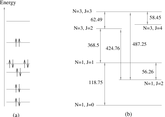
Figure 2: (a) The energy and spin configuration of the 12 valence electrons of the oxygen molecule in its ground state. The two highest energy electrons, which are in the $2\pi_{g}$ orbital, have their spins parallel giving a net spin $S=1$ to the molecule. The lower energy orbitals, which are in order the $1\pi_{g},\,3\sigma_{g},\,2\sigma_{u},\,$ and $1\sigma_{u}$, and the 4 inner shell electrons (not shown) give a net spin of zero. (b) The first two rotational energy levels, N=1 and 3, of the oxygen molecule in the electronic and vibrational ground state. The N and J pairs give the rotational and total angular momentum quantum numbers. The numbers near the arrows give the frequency of the transition in GHz. The Zeeman splitting is not shown.

Radiation propagating through the atmosphere at frequencies near 120 GHz (or near any other oxygen line) will become polarized because of differential polarized absorption and emission by the $\sigma$ and $\pi$ lines.

2.1 Order of Magnitude Estimate

It is not difficult to give an order of magnitude estimate of the polarized intensity of the 118 GHz oxygen line in emission due to the Zeeman splitting. Since we are mainly interested in frequencies at which the atmosphere is not opaque, we can neglect Doppler broadening. We further assume that the line profile is collisional with no mixing, that is Lorenzian. For the 118 GHz line this assumption is valid because the relative strength of the three Zeeman components changes both with polarization and viewing geometry. Any mixing between two transitions is reciprocal in the sense that it acts oppositely on them, and isolation of one transition would imply a non-physical line shape, such as negative absorption. One Zeeman component can not couple to another component that might disappear to a different observer. It can only couple to another component of the same $\Delta M$. (See also the discussion following Eq. 3 of Rosenkranz and Staelin [5].) Hence the emission from the three components is incoherent and we simply sum the Stokes vectors that are associated with each of them

$${{\mbox{\boldmath$S$}}}(\nu,\theta)=\mu_{\pi}L_{\pi}(\nu){{\mbox{\boldmath$S$}}}_{\pi}(\theta)+\mu_{\sigma_{+}}L_{\sigma_{+}}(\nu){{\mbox{\boldmath$S$}}}_{\sigma_{+}}(\theta)+\mu_{\sigma_{-}}L_{\sigma_{-}}(\nu){{\mbox{\boldmath$S$}}}_{\sigma_{-}}(\theta),$$ (1)

where $S$ is the appropriate Stokes vector, $\nu$ is the frequency of interest, $\theta$ is the angle between the line of sight and the direction of the magnetic field, and $\mu$ is the relative strength of the transition, which is proportional to the square of the matrix element between the energy states. The Lorentzian functions are given by

$$L(\nu)=I_{0}{\gamma\over(\nu-\nu_{c})^{2}+\gamma^{2}}$$ (2)

with

$$\nu_{c}=\left\{\begin{array}[]{ll}\nu_{0}&\mbox{for }\pi\\ \nu_{0}-\delta&\mbox{for }\sigma_{+}\\ \nu_{0}+\delta&\mbox{for }\sigma_{-}\end{array}\right.,$$ (3)

where $\nu_{0}$ is the frequency of the $\Delta M=0$ transition, $\delta$ is the magnitude of the shift in frequency, and $I_{0}$ is a normalizing constant proportional to the temperature of the atmosphere. The Stokes vectors of the lines are

$${{\mbox{\boldmath$S$}}}_{\sigma_{\pm}}=\left(\begin{array}[]{c}1+\cos^{2}\theta\\ 1-\cos^{2}\theta\\ 0\\ \pm 2\cos\theta\end{array}\right)$$ (4)

and

$${{\mbox{\boldmath$S$}}}_{\pi}=\sin^{2}\theta\left(\begin{array}[]{c}1\\ -1\\ 0\\ 0\end{array}\right),$$ (5)

and $(\mu_{\pi},\mu_{\sigma_{+}},\mu_{\sigma_{-}})=(2,1,1)$.

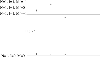
Figure 3: Zeeman splitting of the $(N,J)=(1,1)$ energy level to three levels in the presence of a magnetic field. The $\Delta M=0$ transition is called $\pi$ and the $\Delta M=\pm 1$ transitions are called $\sigma_{\pm}$, where $\Delta M\equiv M-M^{\prime}$.

We estimate the magnitude of the effect for two limiting cases of observation parallel to and perpendicular to the direction of the magnetic field. In the limiting case of an observation parallel to the field, for which $\theta=0$, we have

$${{\mbox{\boldmath$S$}}}_{\sigma_{\pm}}=\left(\begin{array}[]{c}2\\ 0\\ 0\\ \pm 2\end{array}\right)$$ (6)

and the null vector for $S_{\pi}$, which gives two circularly polarized lines from the $\sigma$ components and no $\pi$ component. For the case of observation perpendicular to the field, for which $\theta=\pi/2$, we have

$${{\mbox{\boldmath$S$}}}_{\sigma_{\pm}}=\left(\begin{array}[]{c}1\\ 1\\ 0\\ 0\end{array}\right)$$ (7)

and

$${{\mbox{\boldmath$S$}}}_{\pi}=\left(\begin{array}[]{c}1\\ -1\\ 0\\ 0\end{array}\right)$$ (8)

which gives orthogonal linear polarizations for the $\sigma$ and $\pi$ components.

In the limit where $\gamma,\delta\ll(\nu-\nu_{0})$, which is always the case for altitudes of less than 50 Km above Earth, the polarized intensity for $\theta=\pi/2$ is purely a $Q$ Stokes state and is given by

$$I_{p}(\nu,\theta=\pi/2)=Q(\nu)\simeq{1\over 2}I_{t}\left({\delta\over\nu-\nu_{0}}\right)^{2},$$ (9)

where $I_{t}$ is the total intensity (the I Stokes parameter). The polarized intensity is quadratic in the ratio of $\delta$ to the distance in frequency from line center $\nu-\nu_{0}$. for $\nu=140$ GHz we have $\nu-\nu_{0}=20$ GHz and with $\delta=1$ MHz, corresponding to a field of $\sim 1$ Gauss, and an atmosphere brightness temperature of 10 Kelvin we find $I_{p}\simeq 10\times 10^{-9}$ Kelvin, similar to the estimate of Keating et al. [6].

For the geometry where $\theta=0$ the polarized intensity is purely a $V$ Stokes state, i.e. it is fully circular, but with a much larger amplitude

$$I_{p}(\nu,\theta=0)=V(\nu)\simeq 4I_{t}\left({\delta\over\nu-\nu_{0}}\right).$$ (10)

The polarized intensity is now linear in the ratio of $\delta$ to the distance in frequency from line center. for $\nu=140$ GHz we have $I_{p}\simeq 10^{-3}$ Kelvin. Even a 0.1% conversion of circular polarization to linear in the instrument will give rise to signals that are significant compared to the cosmological signals.

2.2 A More Exact Calculation

The brightness temperature matrix of the atmosphere $\rm{T_{b}}$ at a frequency $\nu$ is given by [4]

$$\rm{T_{b}}(z)=\exp\left\{-\rm{G}(z)\right\}\rm{T_{b}}(0)\exp\left\{-\rm{G}^{*}(z)\right\}+\rm{T_{b}}(0)\left[\rm{I}-\exp\left\{-2\rm{A}(z)\right\}\right],$$ (11)

where $\rm{G}(z)$ is the propagation matrix at a height $z$ above Earth, $\rm{A}$ is the attenuation matrix and $\rm{I}$ is the identity matrix. We use the computer code of Rosenkranz and Staelin [5] to calculate the polarized radiative transfer of the cosmic microwave background radiation through two standard atmospheres [7, 8]: The 1976 US Standard Atmosphere, which is characteristic for latitudes of about 40N with total water vapor of 14 precip. mm, and a winter atmosphere at a latitude of 60N with total water vapor of 4 precip. mm. Magnetic field information comes from the IGRF 1995 magnetic field model [9]. Table  1 gives the effective temperature of each of the stokes parameters (in thermodynamic temperature) at three different frequencies and two altitudes of observations. The observation sites are at a longitude of 140 W and at either 40N or 60N, as appropriate, and observations are pointed toward North at an elevation of 45 degrees. The calculations include contributions due to the 60 GHz oxygen band, for which we calculate the line mixing using the parameters that were measured by Liebe et al. [10]. These measured values of line mixing (and line broadening) correspond to the combination of Zeeman components within each line, and hence are appropriate to the frequencies considered here, which lie far outside the region of Zeeman structure. However, all of the frequencies considered here lie within 90 GHz of the line centers, so duration-of-collision effects are considered to be negligible.

3 Discussion

The results of the calculations using the radiative transfer code and the order of magnitude estimate generally agree and show that the magnitude of the circular polarization is significantly larger than that of the linear polarization component. Although the CMB itself is not expected to be circularly polarized, a 1% conversion of circular to linear polarization in the instrument at a frequency of 90 GHz would give rise to a $3-6\times 10^{-6}$ K signal, depending on the location of observation. Such a signal is of the same order of magnitude as the strongest ’E mode’ signal and much larger than the strongest ’B mode’ signal expected from the CMB, as shown by the bars in Figure 4. However, the Figure also illustrates that the spatial scale where the CMB peaks and the spatial scale that is relevant for the calculation in this paper are quite distinct. (Spatial scales are quantified in terms of $\ell\simeq 180/\theta$, where $\theta$ is the angle between two lines of sight in degrees.) Under the assumption that the atmosphere is well mixed, an assumption that underlies all atmospheric modeling, spatial variations of the atmospheric polarization arise because of variations in the magnetic field along different lines of sight. However, the angular resolution of the IGRF model provides description of spatial variations at $\ell\simeq 1$ for all latitudes except close to the poles. We are currently investigating the magnetic field information close to the poles and at scales smaller than those provided by IGRF and plan to report on it in a future publication.

The polarization of the atmosphere should be considered carefully by ground based experiments that attempt to measure the CMB B mode polarization signal. As Fig. 4 shows, a 0.01% conversion of circular to linear polarization in the instrument gives rise to an atmospheric polarization signal that is larger by $\sim\times 2$ than the largest B signal expected with a cosmology that has a tensor to scalar ratio $r=0.01$. At large angular scales the atmospheric polarization is larger than estimates for the polarization signal due to synchrotron [11] and Galactic dust [12]. Oblique angle reflection of cicularly polarized light from telescope mirrors can readily generate a 0.01% conversion to linear polarization.

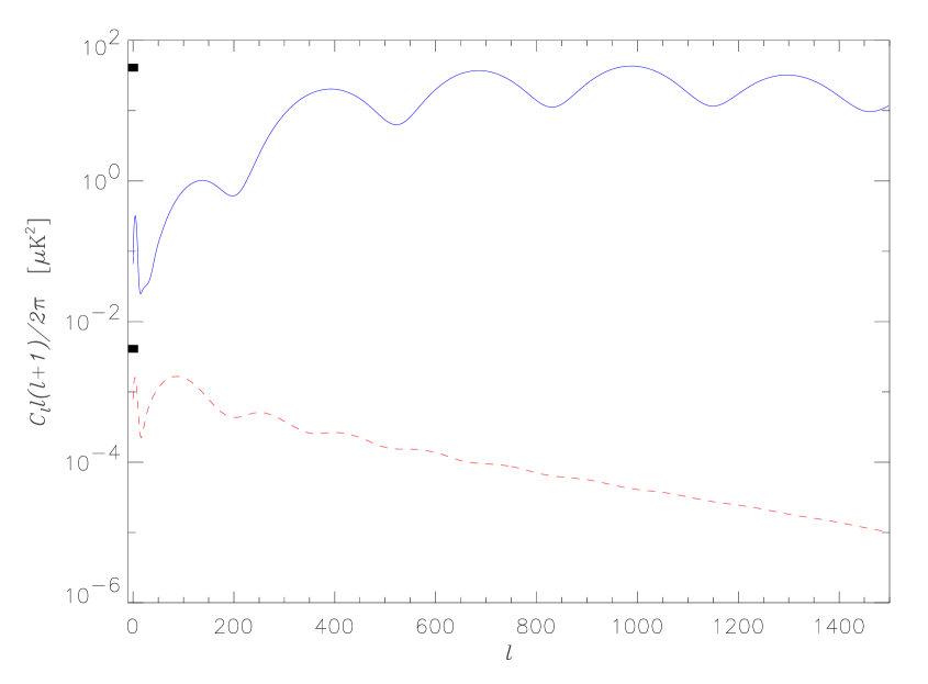
Figure 4: The angular power spectrum of the CMB E (solid) and B (dashed) mode polarization signals in a $\Lambda$CDM cosmology with tensor to scalar ratio $r=0.01$. The top (bottom) short bars near $\ell=0$ show the level of atmospheric polarization at large angular scales that is expected for a 1% (0.01%) conversion of circular to linear polarization in an instrument making observations from the ground at 90 GHz and at a latitude of 60N.

Because the column density of oxygen is much smaller at stratospheric balloon altitudes the signal observed from such a platform is smaller by about a factor of 1000 making it an unimportant foreground for CMB polarization experiments.

The atmospheric polarization signals that we have calculated are valid at a given frequency and have not been integrated over a band of frequencies; Fig. 5 shows the expected variation of the signal as a function of frequency between 125 and 160 GHz for an observation at an altitude of 1 km. We do not give detailed information near the line center at 119 GHz because the line shape is not accurate enough at these frequencies. If the magnitude of the atmospheric polarization at high $\ell$ is the same as that at low $\ell$ then a strong rejection of out of band power will be necessary for ground based polarization experiments.

Figure 5: The $V$ Stokes parameter as a function of frequency for observation through a US standard atmosphere from an altitude of 1 km.

Table 1: Absolute value of the $I$, $Q$, and $V$ Stokes parameters for observation through the atmosphere in Kelvin (thermodynamic units) for observation sites at two latitudes and two altitudes and at the given frequencies. Both sites are at a longitude of 140 W and the observation is toward the North at an elevation of 45 degrees.

Altitude	Frequency	Latitude	I	Q	V
(km)	(GHz)	(deg N)	(K)	(K)	(K)
1	30	40	16	$0.003\times 10^{-6}$	$76\times 10^{-6}$
		60	12	$0.003\times 10^{-6}$	$185\times 10^{-6}$
	90	40	40	$0.02\times 10^{-6}$	$253\times 10^{-6}$
		60	25	$0.02\times 10^{-6}$	$644\times 10^{-6}$
	150	40	81	$0.003\times 10^{-6}$	$23\times 10^{-6}$
		60	35	$0.005\times 10^{-6}$	$78\times 10^{-6}$
30	30	40	2.73	$0.0005\times 10^{-9}$	$15\times 10^{-9}$
		60	2.73	$0.0005\times 10^{-9}$	$28\times 10^{-9}$
	90	40	2.73	$0.005\times 10^{-9}$	$56\times 10^{-9}$
		60	2.73	$0.005\times 10^{-9}$	$102\times 10^{-9}$
	150	40	2.73	$0.001\times 10^{-9}$	$9\times 10^{-9}$
		60	2.73	$0.001\times 10^{-9}$	$16\times 10^{-9}$

Unlike fluctuations in the brightness temperature of the atmosphere, which are primarily due to water clouds at low altitudes the polarized intensity is due to oxygen and is not expected to vary with time, except that it may be attenuated by varying water vapor. For a given observation site the signal will be fixed in a particular azimuth and elevation directions, but not in right ascension and declination.

References

- [1] M. Tinkahm and M. W. P. Strandberg, 1955, “Theory of the Fine Structure of the Molecular Oxygen Ground State”, Phys. Rev. Vol. 97, pgs. 937-951
- [2] M. Tinkham and M. W. P. Strrandberg, 1955, “Interaction of Molecular Oxygen with a Magnetic Field”, Phys. Rev. Vol. 97, pgs. 951-966
- [3] C. H. Townes, and A. L. Schawlow, 1955, “Micorwave Spectroscopy”, McGraw-Hill, New York, 1955.
- [4] W. B. Lenoir, 1968, “Microwave Spectrum of Molecular Oxygen in the Mesosphere” Journal of Geophysical Research, Space Physics, Vol. 73, pgs. 361-376.
- [5] P. W. Rosenkranz and D. H. Staelin, 1988, “Polarized Thermal Microwave Emission from Oxygen in the Mesosphere” Radio Science, Vol. 23, pgs. 721-729.
- [6] B. Keating, P. Timbie, A. Polnarev, and J. Steinberger, 1998, “Large Angular Scale Polarization of the Cosmic Microwave Backgroudn Radiation and the Feasibility of its Detection”, Ap. J. Vol. 495, 580-596.
- [7] “U.S. Standard Atmosphere”, 1976, National Oceanic and Atmospheric Administration, Rockville, published by the US Dept. of Commerce, Natinoal Techcnical Information Service.
- [8] K. F. Kunzi, ed. “Report of Microwave Group on ITRA - Intercomparison Campaign Workshop”, 1987, U. Bern, Switzerland.
- [9] IAGA Division V, Working Group 8, “Revision of International Geomagnetic Reference Field Released”, Eos Trans. AGU, 1996, Vol. 77, pg. 153
- [10] H. J. Liebe, P. W. Rosenkranz, & G. A. Hufford, 1992, “Atmospheric 60 GHz Oxygen Spectrum: New Laboratory Measurements and Line Parameters”, J. Quant. Spectros. Radiat. Transf. Vol. 48, pgs. 629-643.
- [11] G. Giardino, et al., 2002, “Towards a model of full-sky Galactic synchrotron intensity and linear polarisation: A re-analysis of the Parkes data” A & A, Vol. 387, pgs. 82-97
- [12] D. Finkbeiner, M. Davis, & D. Schlegel, 1999, “Extrapolation of Galactic Dust Emission at 100 Microns to Cosmic Microwave Background Radiation Frequencies Using FIRAS” ApJ, Vol. 524, pg. 867.