The evolution of a hot subdwarf: observations of the pulsating subdwarf B star Feige 48

Abstract

Since pulsating subdwarf B (sdBV or EC14026) stars were first discovered (Kilkenny et al, 1997), observational efforts have tried to realize their potential for constraining the interior physics of extreme horizontal branch (EHB) stars. Difficulties encountered along the way include uncertain mode identifications and a lack of stable pulsation mode properties. Here we report on Feige 48, an sdBV star for which follow-up observations have been obtained spanning more than four years, which shows some stable pulsation modes.

We resolve the temporal spectrum into five stable pulsation periods in the range 340 to 380 seconds with amplitudes less then 1%, and two additional periods that appear in one dataset each. The three largest amplitude periodicities are nearly equally spaced, and we explore the consequences of identifying them as a rotationally split $\ell=1$ triplet by consulting with a representative stellar model.

The general stability of the pulsation amplitudes and phases allows us to use the pulsation phases to constrain the timescale of evolution for this sdBV star. Additionally, we are able to place interesting limits on any stellar or planetary companion to Feige 48.

1 Introduction

To date, over 30 pulsating subdwarf B (EC 14026 or sdBV) stars have been identified, with pulsation periods ranging from 68 to 528 seconds and with amplitudes generally less than 50 millimagnitudes (mmag). For recent reviews of this class of stars, see Kilkenny (2001), and Reed, Kawaler & Kleinman (2000), for observational properties; Charpinet, Fontaine & Brassard (2001 and references therein) describe in detail some important aspects of pulsation theory in sdB stars. Most sdBV stars show periods at the short end of the range, and probably represent stars close to the Zero Age Horizontal Branch (ZAHB). PG 1605+072 is the longest period, and lowest gravity, sdBV star, with Feige 48 being an intermediate object. In general, the longer-period sdBV stars represent more highly evolved objects.

Feige 48 was identified as a “faint blue star” as part of the Feige survey (Feige, 1958). It was re-categorized as an sdB star when it was observed as part of the Palomar-Green survey (Green, Schmidt, & Liebert, 1984). Koen et al. (1998; hereafter K98) identified five pulsation periods in Feige 48 in six observing runs from 1997 May to 1998 February. The periods detected by K98 range from 342 to 379 seconds with the largest amplitude being 6.4 mmag. Amplitude variability led K98 to conclude that mode beating was probably present implying that other unresolved modes were present in their data. This provided the motivation for our follow-up observations. Heber, Reid, & Werner (2000; hereafter HRW) obtained a high resolution (0.09Å) spectrum of Feige 48, from which they determined log $g$=5.50$\pm$0.05 and T_eff=29500$\pm$300 K. This makes Feige 48 among the coolest sdBV stars known with a surface gravity intermediate between PG 1605+072 and the rest of the class.

Here we report on our multi-year campaign of high-speed photometry of Feige 48. In Section 2, we outline our observations. Section 3 describes the time series analysis and period identifications. We report on a stellar model fit to Feige 48 in Section 4. The phase stability of pulsations is described in Section 5, where we use this stability to place interesting limits on any possible planetary companion. Section 6 gives our conclusions and outlines future observations for Feige 48.

2 High Speed Photometry

Table 1: Observations of Feige 48

Run	Length	Date	Observatory	Run	Length	Date	Observatory
	(hrs)	UT			(hrs)	UT
tex-007	1.2	1997.03.05	McDonald 0.9m	suh-106	3.2	2000.08.11	Suhora 0.6m
tex-018	2.1	1997.02.06	McDonald 0.9m	jxj-125	2.5	2000.26.11	BAO 0.85m
tex-223	5.7	1998.23.01	McDonald 0.9m	jxj-128	3.2	2000.27.11	BAO 0.85m
tex-236	2.9	1998.28.01	McDonald 0.9m	suh-107	8.8	2000.21.12	Suhora 0.6m
tex-239	5.5	1998.29.01	McDonald 0.9m	suh-108	3.4	2000.22.12	Suhora 0.6m
tex-241	5.9	1998.30.01	McDonald 0.9m	mdr145	8.0	2001.18.01	Fick 0.6m
tex-246	6.7	1998.01.02	McDonald 0.9m	mdr146	8.2	2001.20.01	Fick 0.6m
mdr006	2.2	1998.22.11	McDonald 0.9m	mdr147	3.6	2001.21.01	Fick 0.6m
mdr009	2.6	1998.23.11	McDonald 0.9m	mdr148	9.2	2001.22.01	Fick 0.6m
mdr012	2.6	1998.24.11	McDonald 0.9m	mdr149	9.5	2001.24.01	Fick 0.6m
mdr017	2.8	1998.26.11	McDonald 0.9m	mdr150	9.2	2001.25.01	Fick 0.6m
mdr018	6.0	1999.06.03	McDonald 2.1m	mdr151	7.3	2001.01.02	Fick 0.6m
mdr021	5.5	1999.09.03	McDonald 2.1m	asm-0086	4.4	2001.19.04	McDonald 0.9m
mdr023	4.1	1999.10.03	McDonald 2.1m	sara0082	3.7	2001.21.04	SARA 0.9m
mdr24a	6.0	1999.11.03	McDonald 2.1m	tkw-0065	7.3	2001.22.04	McDonald 0.9m
mdr29a	8.7	1999.15.03	McDonald 2.1m	sara0086	6.8	2001.24.04	SARA 0.9m
mdr030	1.5	1999.17.03	McDonald 0.9m	IAC80A08	0.8	2001.25.04	Teide 0.8m
mdr033	2.0	1999.19.03	McDonald 0.9m	sara0088	7.0	2001.25.04	SARA 0.9m
mdr035	6.0	1999.20.03	McDonald 0.9m	IAC80A09	6.1	2001.26.04	Teide 0.8m
mdr039	5.3	1999.23.03	McDonald 0.9m	sara0089	5.4	2001.26.04	SARA 0.9m
caf48r1r2	7.5	1999.12.04	Calar Alto 1.2m	suh-102	3.9	2001.29.04	Suhora 0.6m
suh-75	1.7	1999.13.04	Suhora 0.6m	suh-103	0.6	2001.30.04	Suhora 0.6m
caf48r3	9.3	1999.13.04	Calar Alto 1.2m	suh-104	0.1	2001.30.04	Suhora 0.6m
mdr091	4.0	1999.10.12	Fick 0.6m	IAC80A17	6.1	2001.30.04	Teide 0.8m
mdr093	6.2	1999.13.12	Fick 0.6m	mdr198	7.0	2002.17.02	Fick 0.6m
mdr095	2.4	1999.14.12	Fick 0.6m	mdr199	1.5	2002.05.04	Fick 0.6m
mdr096	4.9	1999.16.12	Fick 0.6m	mdr200	4.5	2002.06.04	Fick 0.6m
mdr098	2.1	2000.08.02	McDonald 0.9m	suh-109	1.9	2002.07.05	Suhora 0.6m
mdr100	1.3	2000.08.02	McDonald 0.9m	sara141	7.3	2002.07.05	SARA 0.9m
mdr103	4.6	2000.10.02	McDonald 0.9m	suh-110	5.4	2002.08.05	Suhora 0.6m
mdr108	2.7	2000.12.02	McDonald 2.1m	suh-111	1.2	2002.09.05	Suhora 0.6m
mdr110	1.0	2000.12.02	McDonald 2.1m	adg-519	0.7	2002.11.05	Mt.Bigelow 1.5m
mdr111	3.3	2000.28.02	Fick 0.6m	suh-112	1.2	2002.12.05	Suhora 0.6m
mdr112	3.7	2000.01.03	Fick 0.6m	fe0512oh	2.2	2002.12.05	OHP 1.9m
mdr113	4.0	2000.02.03	Fick 0.6m	jr0512	3.4	2002.12.05	Moletai 1.65m
mdr114	1.5	2000.03.03	Fick 0.6m	suh-113	4.4	2002.13.05	Suhora 0.6m
mdr115	6.3	2000.04.03	Fick 0.6m	jr0513	3.7	2002.13.05	Moletai 1.65m
mdr116	2.6	2000.04.03	Fick 0.6m	fe0513oh	1.1	2002.13.05	OHP 1.9m
mdr117	6.0	2000.05.03	Fick 0.6m	jgp0209	0.7	2002.14.05	Teide 0.8m
mdr118	3.3	2000.05.03	Fick 0.6m	jkt-003	1.7	2002.14.05	JKT 1.0m
mdr119	3.8	2000.04.05	Fick 0.6m	jkt-007	5.6	2002.17.05	JKT 1.0m
mdr120	6.0	2000.05.05	Fick 0.6m	a0239	1.0	2002.18.05	McDonald 2.1m
suh-101	6.0	2000.02.11	Suhora 0.6m	jr0518	1.7	2002.18.05	Moletai 1.65m
suh-102	2.9	2000.03.11	Suhora 0.6m	jr0519	2.4	2002.19.05	Moletai 1.65m
suh-103	1.4	2000.05.11	Suhora 0.6m	jr0520	2.2	2002.20.05	Moletai 1.65m
suh-104	9.7	2000.05.11	Suhora 0.6m	jr0521	3.0	2002.21.05	Moletai 1.65m
suh-105	4.6	2000.07.11	Suhora 0.6m

We began observing Feige 48 in 1998 November, with our most recent observations acquired in 2002 May. Table 1 provides a complete list of our observations (including K98’s observations). We acquired most of the data using 3 channel photoelectric photometers as described in Kleinman, Nather, & Phillips (1996). At Fick Observatory, we used a 2 channel photometer of similar design. The Fick data typically have an $\approx$30 minute gap during the night, as the telescope mount requires the photometer to be disconnected when the telescope exchanges sides on the pier. Because this instrument is a 2 channel photometer, the data were occasionally interrupted to measure the sky background. All photometers used Hamamatsu R647 photomultiplier tubes. Data acquired at Calar Alto and SARA were obtained using CCDs with 5 second exposures on a 30 and 15 second duty cycle, respectively. As both the target and comparison star were in the same CCD field, differential photometry removed extinction and sky variation. However, since extinction is wavelength–dependent, colour differences between the stars produced small non-linear trends in the data. We remove these trends by dividing by a low (2 - 4) order polynomial fit to the single–night data. Bad points in the CCD data were removed by hand. No filters were used during any of the photoelectric observations to maximize the photon count rate, whereas the CCD observations used filters to approximate the passband of the Hamamatsu phototubes (Kanaan et al. 2000).

As Table 1 indicates, we have obtained a total of $\approx$380 hours of time series photometry on Feige 48. The data span from 1998 January to 2002 May (the two runs in 1997 were too short and too temporally separated to be useful for this analysis).

3 The Pulsation Spectrum of Feige 48

We follow the standard procedure for determining pulsation frequencies from time series photometry obtained using the Whole Earth Telescope (see, for example, O’Brien et al. 1998). In short, we identify the principal pulsation frequencies with a Fourier transform of light curves of individual nights. We then combine data from several contiguous nights to refine the frequencies. Once the main frequencies are found, we then do a nonlinear least squares fit for the frequencies, amplitudes, and phases of all identified peaks, along with their uncertainties. .

Table 2: Subgroups used in pulsation analysis.

Group	Inclusive dates	Hours of data.
I	1998.28.01 - 1998.01.02	26.7
II	1998.22.11 - 1998.26.11	10.2
III	1999.06.03 - 1999.13.04	63.6
IV	1999.10.12 - 1999.16.12	17.5
V	2000.08.02 - 2000.05.03	42.4
VI	2000.04.05 - 2000.05.05	9.8
VII	2000.02.11 - 2000.22.12	45.7
VIII	2001.18.01 - 2001.01.02	55.0
IX	2001.19.04 - 2001.30.04	52.0
X	2002.05.04 - 2002.21.05	56.8

To work around monthly and annual gaps between observing runs, we begin our analysis of the data in separate, relatively contiguous subgroups. The dates and data hours obtained for the subgroups are given in Table 2, the temporal spectra and window functions for the groups are plotted in Fig. 1. All groups were analysed independently, without using periods detected in other groups. This independent group reductions decrease the likelihood of selecting a daily alias over a real pulsation. Only in our Group X data, do we detect a mode ($f$2) inconsistent with the other group reductions. As such, we presume that our periods for $f1-f5$ are not aliases, with the exception of $f$2 in Group X, which is a daily alias away from the real period. Frequencies determined for the better data sets are in Table 3 with the corresponding temporal spectra of the best groups (Groups III, V, and IX) and the prewhitened residuals in Fig. 2. Though some signal remains in the Fourier transform after prewhitening within these groups, we cannot distinguish any remaining pulsation frequencies from noise.

From our best solution for the Group III data, temporally adjacent groups were added one at a time and frequencies and amplitudes were fit again until a satisfactory fit was determined for all the data. Though there is still a chance that some modes may be off by an annual or monthly alias, the periods, frequencies and amplitudes in Table 4 represent our best solution. Also indicated by Table 3 are three pulsation periods that appear only within the span of a single group. However, the amplitudes are sufficiently low that some possibility exists that they could be due to noise and or aliasing. As such, we will not include them in our analysis, but we mention them as they are possibly stochastically excited modes within an otherwise stable pulsation spectrum. Note also that an error corresponding to an annual (or even monthly) alias produces only a small change in the period or frequency, and so will not affect the modeling for asteroseismic analysis. Such a mistake, however, would be fatal to the period stability analysis.

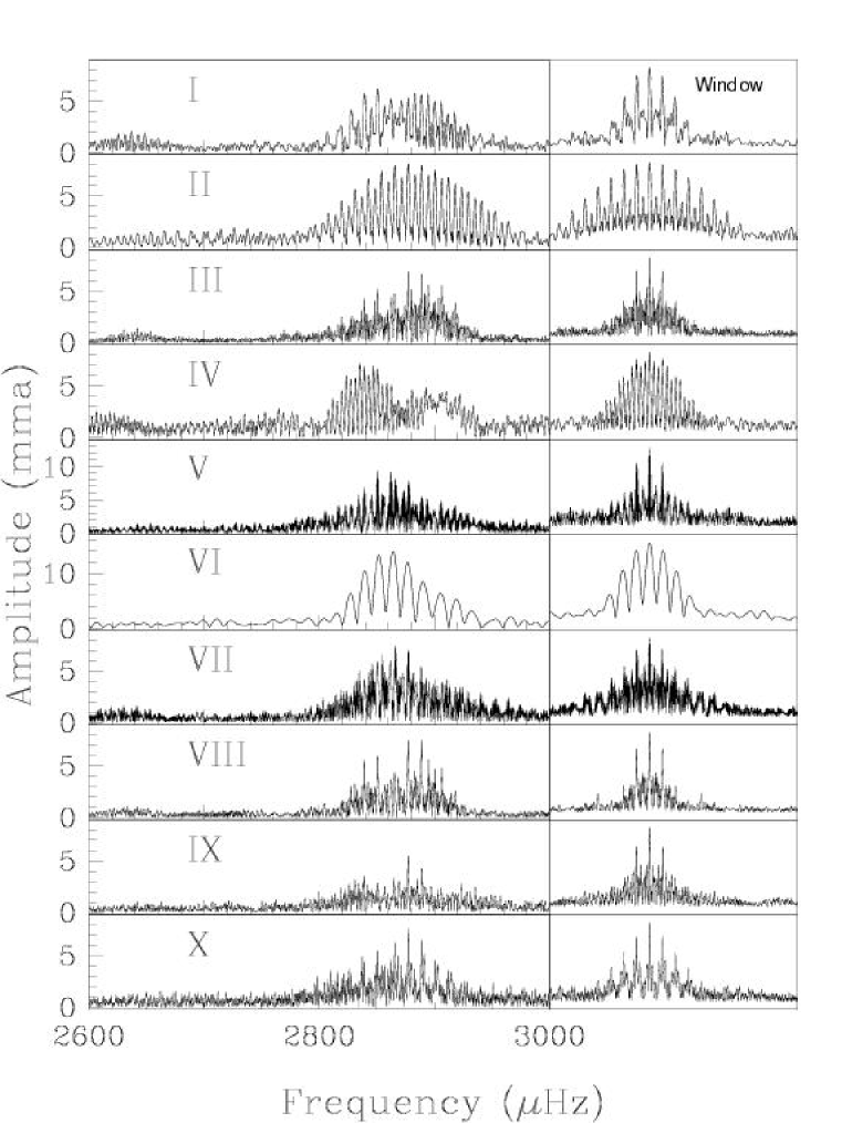
Figure 1: Temporal spectra and Window functions of Feige 48 for the groups listed in Table 2.

Table 3: Comparison of the pulsation frequencies (in $\mu$Hz) detected in various runs. Formal least squares errors are provided in parentheses.

Group	$f1$	$f2$		$f3$		$f4$		$f5$
$\mu$Hz
I†	2636.96(15)			2850.530(40)	2874.40(23)	2877.310(50)		2917.700(70)⋆
III	2641.98(1)	2837.53(1)		2850.833(4)		2877.157(3)		2906.275(4)
V	2641.49(2)	2837.53(1)		2850.833(3)		2877.177(4)	2890.025(19)	2906.299(8)
VIII	2642.00(7)	2837.53(5)		2850.818(17)		2877.153(12)		2906.266(22)
IX	2641.98(6)	2837.78(3)	2841.151(9)	2850.946(26)		2877.185(13)		2906.144(23)
X	2641.86(6)	2826.97(6)⋆		2850.811(12)		2877.220(10)		2906.665(43)
† These frequencies are directly from K98.
⋆ Indicates modes offset by approximately the daily alias (11.56 $\mu$Hz).

Table 4: Least squares solution to the entire data set. Formal least squares errors are in parentheses.

Mode	Period	Frequency	Amplitude
	(sec)	($\mu$Hz)	(mma)
$f1$	378.502960(37)	2641.98731(23)	1.19(6)
$f2$	352.409515(32)	2837.60791(21)	1.30(6)
$f3$	350.758148(3)	2850.96729(7)	4.17(6)
$f4$	347.565033(19)	2877.15942(4)	6.35(6)
$f5$	344.082794(15)	2906.27734(8)	3.57(6)

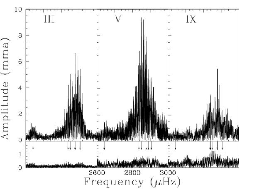
Figure 2: Temporal spectra (top) and residuals after prewhitening by frequencies in Table 4 (bottom).

Feige 48 shows five distinct and consistent pulsation modes. Four of the stable modes cluster with periods near 350 seconds and a single mode lies at 378.5 seconds. The three shortest period modes also have the highest amplitudes – over three times higher than the two longer period modes.

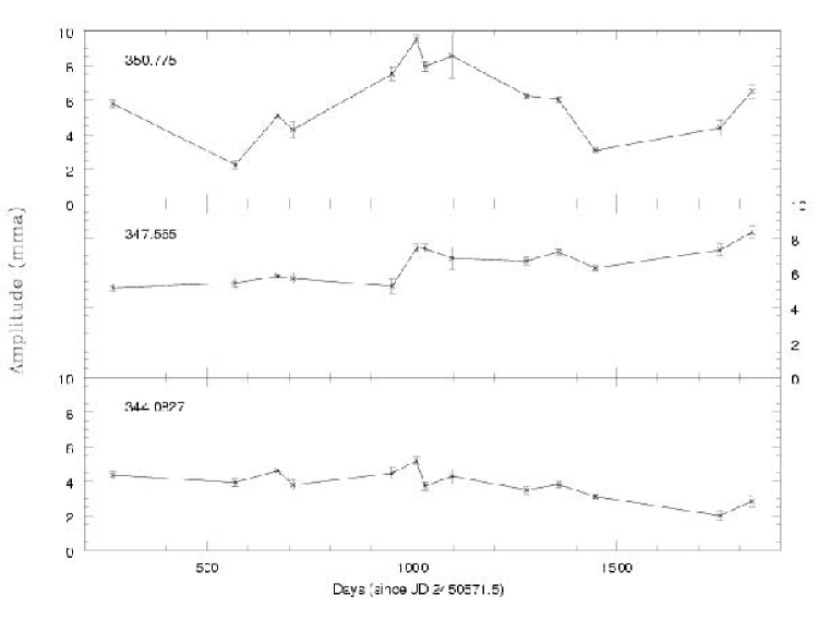
Figure 3: Pulsation amplitudes for the 3 largest amplitude modes.

Our initial interest in follow-up observations of Feige 48 was amplitude variability observed by K98. Our hope was to detect unresolved pulsations that could be responsible for the apparent amplitude variability they reported. However, it appears that the pulsations are resolved, and each has a variable amplitude of at least 30 %. The amplitudes determined for each of our groups for the three high amplitude modes are shown in Figure 3. All 3 amplitudes show change, though only $f3$ has a dramatic degree of variability.

4 Analysis of the pulsation spectrum of Feige 48

4.1 Frequency splittings in Feige 48

For most sdBV stars, sufficient data do not exist to resolve the complete pulsation structure. For stars with resolved temporal spectra (Kilkenny 2001) there are typically too many modes to be accounted for by current pulsation theory unless high $\ell$ values are included (where, by high $\ell$, we mean $\ell\geq 3$). Though higher $\ell$ modes could be present, such modes suffer from severe cancellation effects across the unresolved stellar disk. In any case, identification of rotationally split multiplets ($\ell=1$ triplets or $\ell=2$ quintuplets of nearly equally spaced modes, for example) could aid in accounting for the many modes seen. Unfortunately, previous studies have been limited by a lack of equally spaced (in frequency or period) pulsations as a constraint on the observed $\ell$ values (with the exception of PG 1605+072; Kawaler 1999).

Even though Feige 48 has a relatively simple pulsation spectrum, understanding why this star pulsates with these frequencies still presents a problem. The tight cluster of four modes with periods spanning a range of less than 10 seconds is impossible to accommodate with purely radial pulsation modes in sdB models. Even appealing to nonradial pulsations, the closeness of these periods means that rotation (or other departures from spherical symmetry) must play a role. The reason is that if all are $m$=0 modes, standard evolutionary models of sdB stars at the same $T_{\rm eff}$ and $\log g$ as Feige 48 do not have dense enough frequency spectra to account for these 4 modes, even if one appeals to modes of higher degree than $\ell=3$.

However, Feige 48 may provide important clues in its observed pulsation spectrum. The frequency difference between $f3$ and $f4$ (26.2 $\mu$Hz) is very close to the difference between $f4$ and $f5$ (29.1 $\mu$Hz). Though not exact, this splitting is highly suggestive that $f3$, $f4$, and $f5$ are a rotationally split mode, and probably $\ell=1$. We note that the frequency splitting is not precisely equal (26 versus 29 $\mu$Hz). First order pulsation theory (if applicable here) says that the splitting should be precisely equal – though observations of rotational splitting in white dwarf stars show asymmetries such as this (i.e. in PG 2131, Kawaler et al. 1995 or GD358, Winget et al. 1994).

Another possible clue is that the spacing between $f2$ and $f3$ is 13.2 $\mu$Hz, which is almost exactly half the frequency spacing between $f3$ and $f4$. Thus we could interpret the observed frequencies as follows: the $f3$, $f4$, $f5$ set make an $\ell=1$ triplet, meaning the model needs to fit $f4$ with an $\ell=1$, and $f3$ and $f5$ reveal the rotation rate. Or, $f2$, $f3$, and $f4$ are three components of an $\ell=2$ quintuplet with a spacing of $13.2$ $\mu$Hz. In this case the $m=0$ component could either be $f3$ itself or $f3+13.2$ $\mu$Hz (with a period of 349.1 seconds).

4.2 Comparison with standard evolutionary models

Though we by no means have a complete grid of models and cannot quantify the uniqueness of our results, we can see if either of the above possibilities is consistent with expectations from standard evolutionary models of sdB stars. We take the approach of Kawaler (1999); find a model that first satisfies the spectroscopic constraints of $T_{\rm eff}$ and $\log g$ and that also has pulsation frequencies that match those observed. Further constraining the match is the required value of $\ell$ and $m$ for each possible interpretation of the splittings noted above.

With 5 frequencies available, there are multiple ways to match observations with model frequencies depending on the assumed values of $\ell$, and $m$ for each mode. The most obvious assumption to make is that modes $f3$, $f4$, and $f5$ form a rotationally split triplet with $\ell$=1, $m$=-1,0,+1. This choice has no “missing members” of the multiplet. With this assumption, the model that fits the spectroscopic data must show an $\ell=1$ mode at $f4$, and modes at $f1$ and $f2$. Other choices for this triplet which do require that some components of the multiplet are unobserved are $\ell$=2, with $\Delta m=2$ ($m$=-2,0,+2) or $\Delta m=1$ (e.g. $m$=-2,-1,0 or $m$=-1,0,+1). Similarly, the interpretation of $f2$, $f3$, and $f4$ being components of an $\ell=2$ multiplet, as described above, is viable.

Without choosing a priori one of these interpretations, we examined evolutionary models within our preliminary grid as described below. We generated full evolutionary stellar models using a version of the ISUEVO stellar evolution program (Dehner 1996; Dehner & Kawaler 1995; Kawaler 1999) that incorporates semiconvection in the core helium–burning phase. Our initial grid of evolutionary tracks and models spans the observed range of T_eff and $\log g$ for sdB stars with a core mass of 0.47M_⊙ and solar metalicity. We computed evolutionary tracks for models with hydrogen envelope masses ranging from 0 to 0.00550 M_⊙. From this initial grid, we focused on models whose evolutionary tracks pass within 1$\sigma$ of the spectroscopically determined values of T_eff and $\log g$ (HRW). For these models, we then calculated their pulsation periods to see which (if any) had radial or nonradial pulsation periods near those observed, for any possible choice of $\ell$ and identification of the $m=0$ component of a rotationally split multiplet. For the sequence that most closely matched the observed periods, we iteratively produced models with smaller differences in H shell masses and smaller evolutionary time-steps.

We did find a model that matched the spectroscopic constraints, and could explain four of the five observed frequencies. The closest model fit came from a model in the evolutionary track shown in Fig. 4. This model does an excellent job in explaining $f2$ through $f5$ and requires the identification of $f3$, $f4$, and $f5$ as a rotationally split $\ell=1$ triplet. The model is fairly evolved (as we suspected) and has nearly exhausted its core helium, with only 0.74% (by mass) of the core composed of helium. Table 5 shows a comparison between the observed periods and best-fitting model periods, and the observed spectroscopic properties and the model parameters. With an ad hoc rotational splitting of 27.3$\mu$Hz, this model fits all but the lowest frequency to a precision of 0.2 s. The model temperature agrees to within 150 K, and log $g$ agrees to within 0.02 dex of the measured values; these are well within the $1\sigma$ uncertainties quoted by HRW.

Despite the perception that there are many degrees of freedom, this procedure failed to produce a model that could explain all 5 observed frequencies in terms of normal modes and rotational splitting. Though the model does produce an $\ell$=3, $m$=0 mode at 374 s period, which is near the observed 378 s mode, we currently find no evidence to suggest that Feige 48 has $\ell>2$. Without further evidence (such as other observed members of the multiplet) for invoking high $\ell$ modes, we must confess that our model simply does not reproduce this period without appealing to high $\ell$. Additionally, any $\ell$=2 matches fitted less observed periods. Since we do not have a complete sample of models and this is really just an illustrative example, we are not alarmed. However, it could also indicate that our current models do not include enough physics to be accurate.

The pulsation results for the closest-fitting modes in our best-fitting model series are shown in Fig. 4. Even a small change in log $g$ (as an indication of age) of 0.005 dex changes the calculated periods by more than 3 seconds, worsening the fit to the observations. Likewise, a change in the envelope layer thickness quickly destroys the fit by moving the evolutionary track’s path away from the spectroscopic error box.

Table 5: Comparison of observations with our best-fitting evolutionary model.

	Frequency	Period (sec)		Model
Number	$\mu$Hz	Star	Model	$n$	$l$	$m$
1	2641.99	378.5	(374)	(3)	(5)	(0)
2	2837.60	352.4	352.3	0	0	0
3	2850.83	350.8	350.9	1	1	-1
4	2877.16	347.6	347.4	1	1	0
5	2906.28	344.1	344.3	1	1	+1

	Mass	H shell mass	$T_{\rm eff}$	$\log g$
Spectroscopy			$29500\pm 300$K	$5.50\pm 0.05$
Model	0.4725	0.0025	29635	5.518

4.3 Testing the mode identifications

A test of our (or any) model is the measured constraint on rotational velocity. The observed average rotational splitting of 27.7$\mu$Hz imposed on our $\ell=1$ model identification implies a rotation period of 0.42 days (10 hours). With a radius of 0.20 R_⊙, this model has an equatorial rotation velocity of 24 km  s^-1. To match the constraints of HRW ($v\sin i\leq 5km\cdot s^{-1}$) requires $i\leq 12^{\circ}$. If we use the less restrictive value determined by HRW for only the unblended spectral lines in Feige 48 of $v\sin i\leq 10km\cdot s^{-1}$, our inclination limit increases to $i\leq 25^{\circ}$.

Figure 4: Comparison of the model to the observations. The left panel shows the evolutionary model track (solid line) containing our best-fitting model (dot). The dashed line is the ZAHB and the rectangle is the spectroscopic 1$\sigma$ error box. The right panel compares the model periods (points) to those observed (solid lines). The vertical dashed line indicates the best-fitting model.

The identification of an $\ell=1$ triplet and a radial mode suggest an observation that can be used to test the model. As in white dwarfs (Kepler et al. 2000), time series spectroscopy (particularly in the ultraviolet) should present an effective means of discerning between low and high order ($\ell$) nonradial pulsations. Though it is still in its infancy for sdBV stars (O’Toole et al. 2002; Woolf et al. 2002), if the 378 s period is $\ell$=3, it should be obvious in UV spectroscopy (perhaps less so in the optical) where it should have a significantly higher amplitude than at optical wavelengths. The same is true for our identification of the $\ell$=1 triplet. If any member of our identified triplet really has a different $\ell$ value, the wavelength dependence of its amplitude will be different. Such a test should be obtained as an independent confirmation of our $\ell=1$ determination. While this test can be applied to any sdBV star, Feige 48 has comparatively long pulsation periods (exceeded only by PG 1605+072) and its rather simple temporal spectrum (only 5 periods compared to 55 for PG 1605+072) make it an ideal candidate for time series spectroscopic study.

5 Stability of the pulsation periods

As a star evolves, the pulsation properties evolve in response. In the case of the subdwarf B stars, evolutionary models indicate that they reside on or near the ZAHB for approximately $10^{8}$ years. Upon exhausting their core helium supply, they leave the HB, their $\log g$ goes down, and pulsation periods lengthen. The time scale for evolutionary pulsation period changes (Ṗ/P) after leaving the HB is about 10 times faster than while on the HB.

If Feige 48 has a comparatively small log $g$ because it is a mature HB star that has left the ZAHB, we expect Feige 48 to have an evolutionary Ṗ smaller than PG 1605+072, yet larger than for shorter period pulsators. Since PG 1605+072 does not appear to have pulsations stable enough for an analysis of secular period change caused by evolution (Reed 2001), Feige 48 is the best candidate to examine the $e$-folding time for structural changes caused by its core evolution. As a guide, the model described in Section 4 has a Ṗ=$1.714\cdot 10^{-5}$ s yr^-1. With $\sim$3 years of usable data, the phase of a 350 s period should change by $\sim$14 seconds in that time. This is close to our limit of detection.

To examine long-term phase change, we followed methods outlined in Winget et al. (1985) and Costa & Kepler (2000). First, we obtain a best-fitting least squares fit to all of the periodicities present over the entire span of the observations (Table  4). We then fix the frequencies at these best-fitting values, and recompute the pulsation phases (again via least squares) for each group in Table 2 (note that Groups III and V were divided into two subgroups each because of the long length of the runs). This computed phase represents the observed time of maximum ($O$) for that group, which differs from the computed time ($C$) from the fit to all data. The resulting $O-C$ diagram is shown in Fig. 5 for the three highest amplitude modes (with the pulsation period indicated in each panel). The phase zero point is that defined in K98 as JD=2450571.50.

Fig. 5 shows that the phases are stable throughout most of our observations. Until the Group X data were collected, we believed the Group I data suffered a timing error (proposed in K98). However, it now seems apparent the pulsation modes were only stable over a limited timespan (from Group II through IX). As a check, we analyzed various subgroups of Group X data and reproduced the same phase result. Such a problem is observed in other sdBV stars over a much shorter timescale (Reed 2001). Though we are disappointed in the apparent lack of phase stability, we still have an approximately three year span of phase-stable observations. We therefore used the phase-stable data to place upper limits on the magnitude of Ṗ/P. The combined $O-C$ data of the three highest amplitude modes were weighted and fitted using least squares and give Ṗ/P=$4.9\pm 5.3\times 10^{-16}s^{-1}$. The data are therefore consistent with zero period change and provide a $1\sigma$ lower limit on an evolutionary timescale of $3.1\times 10^{7}$ years. Of course evolution is not the only thing that can drive period changes (see for example Paparó et al. 1998). However, evolutionary models predict that sdBV periods should change in a predictable way (increasing just off the ZAHB, then decreasing after core helium exhaustion, and finally increasing again during shell helium fusion). By measuring Ṗ for several sdBV stars at different stages, we should be able to determine if evolution (as predicted) is driving the period changes.

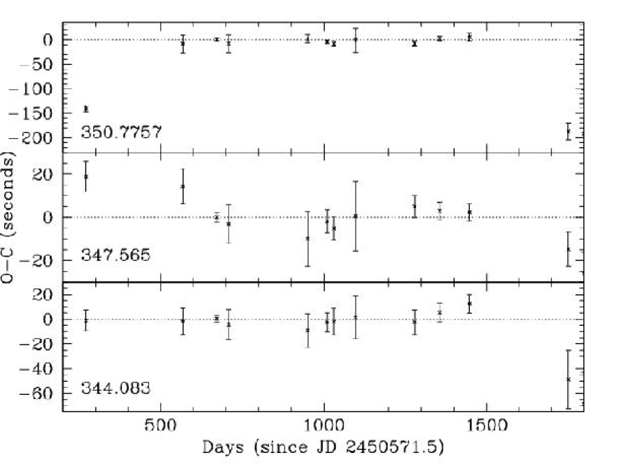
Figure 5: O-C diagrams for the 3 largest amplitude modes.

5.1 $O-C$ variations from reflex orbital motion - planets around Feige 48?

With the phase-stable portion of the data, we can also place useful limits on companions to Feige 48. Orbital reflex motion would create a periodic shift in the pulsation’s arrival time, which would be observed in pulsation phase. Thus any companion must create a periodic phase change within our $O-C$ uncertainties over a scale of days to years. To place limits on companions, we calculated companion mass as a function of binary period and semimajor axis by fitting sine curves (for circular orbits) within our 1, 2, and 3$\sigma$ $O-C$ limits. To assure an upper limit (M$\sin i$) on reflex motion, we use the “noise” in the FT of our $O-C$ as a 1$\sigma$ lower limit: This results in a minimum phase shift of 5 seconds for binary periods under 20 days and 4 seconds for longer periods. Fig. 6 graphically presents our sensitivity to orbital companions. The black, green, and magenta lines are the 1, 2, and 3$\sigma$ limits on M$\sin i$, respectively, while the blue line represents the 3$\sigma$ limit for $i=12^{o}$ (our model constraint). In the short period case (periods under 30 days), the constraint is the limit imposed by the phase errors of individual runs within the data; in the long period case it is the flatness of the $(O-C)$ diagram (including the errors of combined runs) over the phase stable region of our observations. The drop at 30 days corresponds to the change from $O-C$ values determined for single runs to group data sets.

Feige 48 is a horizontal branch star that has lost considerable mass between the red giant branch and its current evolutionary state. Any companion separated by more than $\sim$1 AU is far enough away that common–envelope evolution (or vaporisation) has been avoided. In addition, the orbital separation will have roughly doubled as Feige 48 lost approximately half its mass during the red giant phase. This should produce two cases for binaries: Close stellar companions with original separations $\leq 1$AU will produce a short period binary (which have periods on order of weeks or less) after a common envelope phase. Companions distant enough to avoid a common envelope phase (or vaporisation) will have orbital periods on the order of a year or more. The two panels of Fig. 6 reflect this duality (though it does cover all periods between 2 days and 5 years).

The left panel of Fig. 6 indicates our limits on stellar companions. Our 1$\sigma$ limit is less than 0.1M${}_{\odot}\sin i$ for a binary period of 3 days. The right panel shows our limits on sub–stellar companions. Our “average” 3$\sigma$ limit for $i=12^{o}$ is $\approx 12$M_ψ, while our best 1$\sigma$ limit would detect Jupiter at a period of 2.5 years. Our data are currently sensitive to the extra solar “warm Jupiter” type planets being detected at a distance of 0.6 - 3.0 AU. Planets with orbital separations less than $\sim$1 AU would not have survived the red giant phase. Our data do not rule out a companion in an extremely short period binary or at low inclination.

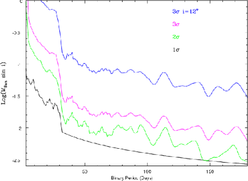
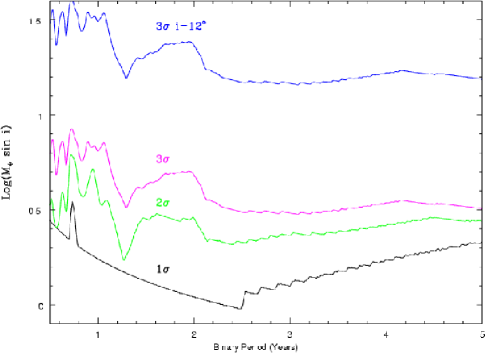
Figure 6: 1$\sigma$, 2$\sigma$, and 3$\sigma$ upper limits on any companions to Feige 48. The time axis is continuous between panels, but changes scale from days to years. The mass axis is discontinuous between panels as the left panel is in solar masses and the right panel has units of Jupiter masses.

6 Conclusions

From our multi-season photometry of Feige 48, we have consistently detected five pulsation periods. Of these five, three ($f$1, $f$3 and $f$4) are consistent with K98. One frequency ($f$5) differs by a daily alias, while K98’s fifth frequency (2874 $\mu$Hz) is not detected in our data. In data sets V and IX, we also detect new pulsation frequencies at 2890 and 2843 $\mu$Hz respectively, indicating that there may be some stochastically excited pulsations in Feige 48. This is consistent with pulsation behavior seen in another sdBV star, PG 1605+072 (Reed 2001).

Our attempted model fit follows the strategy that has been successfully applied to other classes of pulsating stars, but has rarely worked for sdBV stars; namely using observed frequency splittings to impose $\ell$ constraints on models. Using standard evolutionary models, our preliminary model grid includes a model that is able to explain all but the lowest frequency stable pulsations. Most exciting is the fact that such standard models fail to explain all five frequencies. Thus, despite its relative simplicity and the richness of the parameters available, the failure of this model suggests that standard stellar evolution theory does not fully explain the evolution of sdB stars and or the nature of pulsations within them. We have something new to learn.

Our modeling example shows that Feige 48 should also serve as an interesting test for other methods of mode identification. Though optical multicolour photometry was not useful for identifying pulsation modes in KPD2109+4401(Koen 1998), we expect that UV multicolour photometry as developed by Robinson, et al. (1995), will be useful to determine if high–order $\ell$ modes are present in sdBV stars (as indicated by Brassard et al. 2001 and Billères et al. 2000). The argument for high–order $\ell$ values is particularly interesting in light of the frequencies detected in Group V’s data. If the lowest frequency mode is disregarded, the remaining modes have frequency spacings of 13.3, 26.4, 12.8, and 16.3 $\mu$Hz respectively. If these were all parts of a single, rotationally split mode, it would require $\ell\geq 3$. Such an $\ell$ value should be apparent in UV multicolour photometry (see, for example, Kepler et al 2000). As such, we look forward to the analysis of HST data obtained by Heber (2002). Should Heber’s (2002) HST data agree with our $\ell$=1 interpretation, Feige 48 would make an excellent star to calibrate other mode identification methods in sdBV stars such as optical time-series spectroscopy (O’Toole et al 2002; Woolf et al 2002).

The results of our $O-C$ analysis are consistent with a non-binary nature for the star within the data limits. It also indicates that using the $O-C$ diagram to detect planets around evolved stars is possible, though in this case we did not detect any. We plan to continue to monitor Feige 48 over the next several years to tighten the constraints on planetary companions.

Our limit on a stellar companion also addresses the origin of sdB stars. Binary evolution is a candidate for producing sdB stars, either through common-envelope evolution (Sandquist, Taam & Burkert 2000; Green, Liebert & Saffer 2000) or via Roche-lobe overflow near the tip of the red giant branch (Green, Liebert & Saffer 2000). Though observations indicate that a great many sdB stars are in binaries (Reed & Steining 2003; Green, Liebert & Saffer 2000; Han et al 2002), either the evolutionary sequence that produces sdB stars is independent of binary evolution (D’Cruz et al 1996), is bimodal, or has several paths that can result in the production of an sdB star (perhaps including the merger of two low mass white dwarfs as described by Iben & Tutukov 1986). For the case of Feige 48, it would appear that it is either in a short period binary (whose orbital period is commensurate with the $\sim$10 hour rotation period predicted with our model), in a long period binary with an orbital period substantially longer than our data (which would rule out Roche-lobe overflow, so the companion would have no effect on the evolution of the pre-sdB star), in a binary with an extremely low inclination or a single star.

7 acknowledgments

M.D. Reed was partially funded by NSF grant AST9876655 and by the NASA Astrophysics Theory Program through grant NAG-58352 and would like to thank the McDonald Observatory TAC for generous time allocation. S. Dreizler, S.L. Schuh and J.L. Deetjen (Visiting Astronomers at the German-Spanish Astronomical Centre, Calar Alto, operated by the Max-Planck-Institut for Astronomy, Heidelberg, jointly with the Spanish National Commission for Astronomy) acknowledge travel grant DR 281/10-1 from the Deutsche Forschungsgemeinschaft. P. Moskalik is supported in part by Polish KBN grant 5 P03D 012 020.

References

- [1] Billéres M., Fontaine G., Brassard P. Charpinet S., Liebert James, Saffer R. A. 2000, ApJ 530, 441
- [2] Brassard P., Fontaine G., Billéres M., Charpinet S., Liebert James, Saffer R. A. 2001, ApJ 563, 1013
- [3] Charpinet S., Fontaine G,. Brassard P. 2001, PASP, 113, 775
- [4] Costa J.E.S., Kepler S.O., 2000, BaltA, 9, 451
- [5] D’Cruz N.L., Dorman B., Rood R.T., O’Connell R.W., 1996, ApJ, 466, 369
- [6] Dehner B.T. 1996, Ph.D. dissertation, Iowa State University.
- [7] Dehner B.T., Kawaler S.D. 1995, ApJ 445, 141
- [8] Feige J., 1958, ApJ, 128, 267
- [9] Green E. M., Liebert J., Saffer R. A., 2001, in Provencal J.L, Shipman H.L., MacDonald J., and Goodchild S. eds., Proc. 12th European Conference on White Dwarfs, Astron. Soc. Pac., San Francisco, p. 192
- [10] Green R.F., Schmidt M., Liebert J., 1986, ApJ, 61, 305
- [11] Han Z., Podsiadlowski Ph, Maxted P.F.L., Marsh T.R., Ivanova N., 2002, MNRAS, 336, 449
- [12] Heber U, Reid N.I, Werner K. 1999, A&A, 348, L25
- [13] Heber U. 2002, private communication
- [14] Iben I. Jr., Tutukov A.V., 1986, ApJ 311, 753
- [15] Kanaan A., O’Donoghue D., Kleinman S.J., Krzesinski J., Koester D., Dreizler S., 2000, BaltA, 9, 387
- [16] Kawaler, S.D. et al. (the WET Collaboration), 1995, ApJ, 450, 350.
- [17] Kawaler S.D., 1999, in Solheim J.E., Meistas E.G., eds., Proc. 11th European Workshop on White Dwarfs, Astron. Soc. Pac., San Francisco, p. 158
- [18] Kepler S.O., Robinson E.L., Koester D, Clemens J.C., Nather R.E., Jiang X.J., 2000, ApJ 539, 379
- [19] Kilkenny D., Koen C., O’Donoghue D., Stobie R.S., 1997, MNRAS, 285, 640
- [20] Kilkenny D., 2001, in Aerts C., Bedding T.R., Christensen-Dalsgaard J. eds., Proc. IAU Coll. 185, Radial and Nonradial Pulsations as Probes of Stellar Physics, Astron. Soc. Pac., San Francisco, p. 356
- [21] Kleinman S.J., Nather R.E., Phillips T., 1996, PASP, 108, 356
- [22] Koen C., 1998, MNRAS, 300, 567
- [23] Koen C., O’Donoghue D., Pollacco D.L., Nitta A., 1998, MNRAS, 300, 1105.
- [24] O’Brien et al. (the WET collaboration), 1998, ApJ, 495, 458
- [25] O’Donoghue D., Koen C., Kilkenny D., Stobie R.S., Lynas-Gray A.E., 1999, in Solheim J.E., Meistas E.G., eds., Proc. 11th European Workshop on White Dwarfs, Astron. Soc. Pac., San Francisco, p. 149
- [26] O’Toole S.J., Bedding T.R., Kjeldsen H., Dall T.H., Stello D. 2002, MNRAS, 334, 4710
- [27] Paparó M., Saad S.M., Szeidl B., Kolláth Z., Abu Elazm M.S., and Sharaf M.A., 1998, A&A, 332, 101
- [28] Reed M.D., & Steining R., 2003, in preparation
- [29] Reed M.D., 2001, Ph.D. dissertation, Iowa State University.
- [30] Reed M.D., Kawaler S.D., Kleinman S.J., 2000, in Szabados L, Kurtz, D.W. eds., Proc. IAU Coll. 176, The Impact of Large-Scale Surveys on Pulsating Star Research, Astron. Soc. Pac., San Francisco, p. 503
- [31] Robinson E.L, Mailloux T.M., Zhang E., Koester D., Stiening R.F., Bless R.C., Percival J.W., Taylor M.J., van Citters G.W., 1995, ApJ 438, 908
- [32] Sandquist E.L., Taam R.E., Burkert A., 2000, ApJ 533, 984
- [33] Winget D.E., Robinson E.L, Nather R.E., Kepler S.O, O’Donoghue D., 1985, ApJ, 292, 606
- [34] Winget, D.E. et al. (the WET collaboration), 1994, ApJ, 430, 839
- [35] Woolf V.M., Jeffery C.S., Pollacco D.L., 2002, MNRAS, 332, 34