Metallicity of the Intergalactic Medium Using Pixel Statistics.
II. The Distribution of Metals as Traced by C IV

Abstract

We measure the distribution of carbon in the intergalactic medium as a function of redshift $z$ and overdensity $\delta$. Using a hydrodynamical simulation to link the H I absorption to the density and temperature of the absorbing gas, and a model for the UV background radiation, we convert ratios of C IV to H I pixel optical depths into carbon abundances. For the median metallicity this technique was described and tested in Paper I of this series. Here we generalize it to reconstruct the full probability distribution of the carbon abundance and apply it to 19 high-quality quasar absorption spectra. We find that the carbon abundance is spatially highly inhomogeneous and is well-described by a lognormal distribution for fixed $\delta$ and $z$. Using data in the range $\log\delta=-0.5-1.8$ and $z=1.8-4.1$, and a renormalized version of the Haardt & Madau (2001) model for the UV background radiation from galaxies and quasars, we measure a median metallicity of $[{\rm C}/{\rm H}]=-3.47_{-0.06}^{+0.07}+0.08_{-0.10}^{+0.09}(z-3)+0.65_{-0.14}^{+0.10}(\log\delta-0.5)$ and a lognormal scatter of $\sigma([{\rm C}/{\rm H}])=0.76_{-0.08}^{+0.05}+0.02_{-0.12}^{+0.08}(z-3)-0.23_{-0.07}^{+0.09}(\log\delta-0.5)$. Thus, we find significant trends with overdensity, but no evidence for evolution. These measurements imply that gas in this density range accounts for a cosmic carbon abundance of $[{\rm C}/{\rm H}]=-2.80\pm 0.13$ ($\Omega_{\rm C}\approx 2\times 10^{-7}$), with no evidence for evolution. The dominant source of systematic error is the spectral shape of the UV background, with harder spectra yielding higher carbon abundances. While the systematic errors due to uncertainties in the spectral hardness may exceed the quoted statistical errors for $\delta<10$, we stress that UV backgrounds that differ significantly from our fiducial model give unphysical results. The measured lognormal scatter is strictly independent of the spectral shape, provided the background radiation is uniform. We also present measurements of the C III/C IV ratio (which rule out temperatures high enough for collisional ionization to be important for the observed C IV) and of the evolution of the effective Ly$\alpha$ optical depth.

1. Introduction

The enrichment of the intergalactic medium (IGM) with heavy elements provides us with a fossil record of past star formation, as well as a unique laboratory to study the effects of galactic winds and early generations of stars. With the advent of the HIRES spectrograph on the Keck telescope it rapidly became clear that a substantial fraction of the high column density ($N_{\rm HI}\gtrsim 10^{14.5}~{}{\rm cm}^{-2}$) Ly$\alpha$ absorption lines seen at redshift $z\sim 3$ in the spectra of distant quasars have detectable associated absorption by C IV (Cowie et al. 1995; Ellison et al. 2000) and Si IV (Songaila & Cowie 1996). More recently, observations with the UVES instrument on the Very Large Telescope (VLT), as well as with the Keck Telescope, have revealed that the same is true for O VI at $z\sim 2$ (Carswell, Schaye, & Kim 2002; Simcoe et al. 2002; Bergeron et al. 2002, see also Telfer et al. 2002). Both simple photoionization models (e.g., Cowie et al. 1995; Songaila & Cowie 1996; Carswell et al. 2002; Bergeron et al. 2002) and numerical simulations assuming a uniform metallicity (Haehnelt et al. 1996; Rauch et al. 1997a; Hellsten et al. 1997; Davé et al. 1998) indicate that the gas has a typical metallicity of $10^{-3}$ to $10^{-2}$ solar.

The gas in which metals can be detected directly is thought to be significantly overdense [$\delta\equiv\rho/\left<\rho\right>\sim 10~{}(N_{\rm HI}/10^{15}~{}{\rm cm}^{-2})^{2/3}[(1+z)/4]^{-3}$; Schaye 2001] and consequently fills only a small fraction of the volume. The typical metallicity of the low-density IGM (away from local sources of metals) remains largely unknown, although statistical analyses based on pixel optical depths do indicate that there is C IV (Cowie & Songaila 1998; Ellison et al. 2000) and O VI (Schaye et al. 2000a) associated with the low-column density Ly$\alpha$ forest.

Despite the recent progress, many questions remain regarding the distribution of metals in the IGM: Are metals generally present at $\delta\ll 10$? Does the metallicity vary with overdensity? Does the metallicity vary with redshift? How much scatter is there in the metallicity for a fixed density and redshift? Does this scatter change with density or redshift? Are the metals photoionized or does collisional ionization dominate? How does the metallicity change with the assumed spectral shape of the UV-background? What are the relative abundances of the different elements? Except for the last, which we will address in future publications, this paper will address all of these questions.

We measure the distribution of carbon in the IGM by applying an extension of the pixel optical depth method, which we developed and tested in Aguirre, Schaye, & Theuns (2002, hereafter Paper I) — which was itself an extension of the earlier work by Cowie & Songaila (1998) (see also Songaila 1998, Ellison et al. 2000, and Schaye et al. 2000a) — to a set of high-quality quasar spectra taken with the Keck and VLT telescopes. The basic idea is to measure the distribution of C IV pixel optical depths as a function of the corresponding H I optical depth, corrected for noise and absorption by other transitions, and to convert this correlation into an estimate of the metallicity as a function of the density. Our method differs in two respects from that proposed in Paper I: (1) we measure the full distribution of metals instead of just the median metallicity and (2) we correct for noise and contamination using the data themselves instead of simulations. Furthermore, we use the C III/C IV ratio to set an upper limit on the temperature of the enriched gas, ruling out collisional ionization as the dominant ionization mechanism.

This paper is organized as follows. In §2 we describe our sample of quasar spectra, and in §3 we use this sample to measure the evolution of the mean absorption, which we need to normalize the intensity of our UV background models. Before describing these models in §4.2, we briefly describe our hydrodynamical simulation in §4.1. The simulation is used to compute the gas density and temperature as a function of the H I optical depth, which are needed to compute the ionization correction factors, as discussed in detail in §4.3. In §5 we provide a step-by-step description of our method for measuring the median metallicity (§5.1) and the distribution of metals at a fixed density (§5.2). To make the reading more interesting, we illustrate the method by presenting results for one of our best quasar spectra. Section 6 contains our measurements of the C III/C IV ratio, which support our assumption that the temperature is low enough for collisional ionization of C IV to be unimportant. In §7 we present our measurements of the distribution of carbon as a function of overdensity and redshift. In §7.1 we show how the results change if we vary the UV background. In §8 we discuss the results, compute mean metallicities and filling factors, compare with previous work, and estimate the size of systematic errors. Finally, we summarize our conclusions in §9.

How should this paper be read? Given the length of the paper, we encourage reading the conclusions (§9) first. Readers who are not interested in the details of the method would in addition only need to read §§7 and 8. Those who would like to understand the method, but are not interested in knowing all of the details, would benefit from also reading §§4.2, 4.3, and 5. Readers who would like to know more about the mean absorption or the constraints on the ionization mechanism may want to read §§3 and 6, respectively.

2. Observations

We analyzed spectra of the 19 quasars listed in the first column of Table 2. Fourteen spectra were taken with the UV-Visual Echelle Spectrograph (UVES; D’Odorico et al. 2000) on the VLT and five were taken with the High Resolution Echelle Spectrograph (HIRES; Vogt et al. 1994) on the Keck telescope (see col. [7] of Table 2). The UVES spectra were taken from the ESO archive. Only spectra that have a signal-to-noise ratio (S/N) $\gtrsim$ 40 in the Ly$\alpha$ region and that were publicly available as of 2003 January 31 were used. The UVES spectra were reduced with the ESO-maintained MIDAS ECHELLE package (see Kim, Cristiani, & D’Odorico 2001 and Kim et al. 2003 for details on the data reduction). The reduction procedures for the HIRES spectra are described in Barlow & Sargent (1997). The spectra have a nominal velocity resolution of $6.6~{}{\rm km}\,{\rm s}^{-1}$ (FWHM) and a pixel size of 0.04 and 0.05 Å for the HIRES and UVES data, respectively.

For a quasar at redshift $z_{\rm em}$ (the emission redshift), we analyze data in the redshift range $(1+z_{\rm em})\lambda_{{\rm Ly}\beta}/\lambda_{{\rm Ly}\alpha}-1<z<z_{\rm em}-(1+z_{\rm em})\Delta v/c$, where $\Delta v=\max(4000,8\,{\rm Mpc}\,H(z)/h)~{}{\rm km}\,{\rm s}^{-1}$ and $H(z)$ is the Hubble parameter at redshift $z$ extrapolated from its present value ($H_{0}\equiv 100h~{}{\rm km}\,{\rm s}^{-1}\,{\rm Mpc}^{-1}$) assuming $(\Omega_{m},\Omega_{\Lambda})=(0.3,0.7)$. The lower limit ensures that Ly$\alpha$ falls redwards of the quasar’s Ly$\beta$ emission line, thereby avoiding confusion with the Ly$\beta$ forest. The region close to the quasar is excluded to avoid proximity effects. The minimum, median, and maximum absorption redshifts considered are listed in columns (3), (4), and (5) of Table 2.

Regions thought to be contaminated by absorption features that are not present in our simulated spectra were excluded. Examples are absorption by metal lines other than C III, C IV, Si III, Si IV, O VI, N V, and Fe II, and atmospheric lines. Seven spectra (Q1101-264, Q1107+485, Q0420-388, Q1425+604, Q2126-158, Q1055+461, and Q2237-061) contain Ly$\alpha$ lines with damping wings (i.e., $N({\rm HI})\gtrsim 10^{19}~{}{\rm cm}^{-2}$). Regions contaminated by these lines or their corresponding higher order Lyman series lines were also excluded. For the case of damped Ly$\alpha$ lines the excluded regions can be large (up to several tens of angstroms). Contaminating metal lines were identified by eye by searching for absorption features corresponding to the redshifts of strong H I lines and to the redshifts of the absorption systems redward of the quasar’s Ly$\alpha$ emission line (trying a large number of possible identifications). Due to the robustness of our method, which uses the C IV doublet to correct for contamination and is based on nonparametric statistics, our results are nearly identical if we do not remove any of the contaminating metal lines.

Table 1Observed quasars

QSO	$z_{\rm em}$	$z_{\rm min}$	med($z$)	$z_{\rm max}$	$\lambda_{\rm min}$ (Å)	Instrument	Reference
Q1101-264	2.145	1.654	1.878	2.103	3050.00	UVES	1
Q0122-380	2.190	1.691	1.920	2.147	3062.00	UVES	2
J2233-606	2.238	1.732	1.963	2.195	3055.00	UVES	3
HE1122-1648	2.400	1.869	2.112	2.355	3055.00	UVES	1
Q0109-3518	2.406	1.874	2.117	2.361	3050.00	UVES	2
HE2217-2818	2.406	1.874	2.117	2.361	3050.00	UVES	3
Q0329-385	2.423	1.888	2.133	2.377	3062.00	UVES	2
HE1347-2457	2.534	1.982	2.234	2.487	3050.00	UVES	1,2
PKS0329-255	2.685	2.109	2.373	2.636	3150.00	UVES	2
Q0002-422	2.76	2.173	2.441	2.710	3055.00	UVES	2
HE2347-4342	2.90	2.291	2.569	2.848	3428.00	UVES	2
Q1107+485	3.00	2.375	2.661	2.947	3644.36	HIRES	4
Q0420-388	3.123	2.479	2.774	3.068	3760.00	UVES	2
Q1425+604	3.20	2.544	2.844	3.144	3736.20	HIRES	4
Q2126-158	3.268	2.601	2.906	3.211	3400.00	UVES	2
Q1422+230	3.62	2.898	3.225	3.552	3645.24	HIRES	4
Q0055-269	3.655	2.928	3.257	3.586	3423.00	UVES	1
Q1055+461	4.12	3.320	3.676	4.033	4586.36	HIRES	5
Q2237-061	4.558	3.690	4.070	4.451	4933.68	HIRES	4

References. — (1) Kim et al. 2002; (2) Kim et al. 2003; (3) Kim, Cristiani, & D’Odorico 2001; (4) Rauch et al. 1997; (5) Boksenberg, Sargent, & Rauch 2003

3. The observed evolution of the mean Ly$\alpha$ absorption

Our measurements of the effective optical depth, $\tau_{\rm eff}\equiv\left<-\ln F\right>$, where $F$ is the normalized flux in the Ly$\alpha$ forest, are plotted as a function of redshift in Fig. 1 and are listed in Table 1 in Appendix B. Besides the quasars listed in Table 2, we measured $\tau_{\rm eff}$ for two additional HIRES quasar spectra from the Rauch et al. (1997) sample: Q1442+293 ($z_{\rm em}=2.67$) and Q0000-262 (${}_{\rm em}=4.11$). These spectra are not part of our main sample because they do not have sufficient coverage to be useful for our metal analysis. Each Ly$\alpha$ forest spectrum was divided in two, giving 42 data points in total. The left-hand panel shows the results obtained using all pixels in the Ly$\alpha$ forest range; the right-hand panel shows the results obtained after removing all pixels that are thought to be contaminated by metal lines, H I lines with damping wings, and atmospheric lines. Comparison of the two panels shows that removing the contamination generally reduces both the mean absorption and the scatter in the absorption at a given redshift, particularly at lower redshifts.

The dotted lines show least-squares power-law fits to the data points. Note that the scatter is much larger than expected given the error bars: the $\chi^{2}/$dof is about 5.2 and 2.4 for the left- and right-hand panels respectively (for 40 dof). This probably indicates that most of the remaining scatter is due to cosmic variance (see also Kim et al. 2002).

The dashed curve in Figure 1 indicates the evolution of the Ly$\alpha$ optical depth measured by Bernardi et al. (2003), who applied a novel $\chi^{2}$ minimization technique to 1061 low-resolution QSO spectra (their S/N ¿ 4 sample) drawn from the Sloan Digital Sky Survey database. The Bernardi et al. fit gives absorption systematically higher by about 0.1 dex than we obtain from our high-resolution spectra. For $z\gtrsim 3$ our local continuum fits may underestimate the absorption and the Bernardi et al. results may be more reliable. However, for lower redshifts the continuum is well-defined and our results may be more accurate than those of Bernardi et al., whose spectra have insufficient resolution to allow for the identification and removal of metal lines.

Figure 1.— Observed effective optical depth as a function of redshift for all pixels (left-hand panel) and after removal of pixels contaminated by metal lines, Ly$\alpha$ lines with damping wings, or atmospheric lines (right-hand panel). Horizontal error bars indicate redshift ranges used, vertical error bars are 1$\sigma$ errors measured by bootstrap resampling the spectra using chunks of 100 pixels. The solid curve shows the average effective optical depth in the simulated spectra; the dotted lines are power-law least-squares fits to the data points: $\log\tau_{\rm eff}=\log\tau_{0}+\alpha\log[(1+z)/4]$. The best-fit values are $(\log\tau_{0},\alpha)=(-0.40\pm 0.02,3.40\pm 0.23)$ and $(-0.44\pm 0.01,3.57\pm 0.20)$ for the left- and right-hand panels, respectively. The errors on the parameters of the fit were estimated by bootstrap resampling the data points. The dashed curve indicates the evolution of the Ly$\alpha$ optical depth measured by Bernardi et al. (2003) using a $\chi^{2}$ minimization technique on QSO spectra (their S/N ¿ 4 sample) drawn from the Sloan Digital Sky Survey database.

4. Simulation and ionization corrections

Because the C IV optical depth can tell us only about the density of C IV ions, we need to know the fraction of carbon that is triply ionized to determine the density of carbon. The ionization balance depends on the gas density, temperature, and the ambient UV radiation field. We use (variants of) the models of Haardt & Madau (2001) for the UV background and a hydrodynamical simulation to compute the density and temperature as a function of the H I optical depth. Before explaining how we convert the C IV/H I optical depth into a metallicity in §4.3, we will briefly describe our simulation and our method for generating synthetic spectra in §4.1 and our models for the metagalactic UV radiation in §4.2.

4.1. Generation of synthetic spectra

We use synthetic absorption spectra generated from a hydrodynamical simulation for two purposes: (1) to determine the gas density and temperature (which are needed to compute the ionization corrections) as a function of the H I optical depth and redshift and (2) to verify that simulations using the carbon distribution measured from the observed absorption spectra do indeed reproduce the observed optical depth statistics.

The simulation that we use to generate spectra is identical to the one used in Paper I, and we refer the reader to §3 of that paper for details. Briefly, we use a smoothed particle hydrodynamics code to model the evolution of a periodic, cubic region of a $(\Omega_{m},\Omega_{\Lambda},\Omega_{b}h^{2},h,\sigma_{8},n,Y)=(0.3,0.7,0.019,0.65,0.9,1.0,0.24)$ universe of comoving size $12\,h^{-1}~{}{\rm Mpc}$ to redshift $z=1.5$ using $256^{3}$ particles for both the cold dark matter and the baryonic components. The gas is photoionized and photoheated by a model of the UV background, designed to match the temperature-density relation measured by Schaye et al. (2000b). Since we recalculate the ionization balance of the gas when computing absorption spectra, this choice of UV background only affects the thermal state of the gas.

The software used to generate the simulated spectra is also described in detail in Paper I (§3). Briefly, many sight lines through different snapshots of the simulation box are patched together to create long sight lines spanning $z=1.5$ to $z_{\rm em}$. Absorption from Ly1 ($\lambda$1216), Ly2 ($\lambda$1026), …, Ly31 ($\lambda$913), C III ($\lambda$977), C IV ($\lambda\lambda$1548,1551), N V ($\lambda\lambda$1239,1243), O VI ($\lambda\lambda$1032,1038), Si III ($\lambda$1207), Si IV ($\lambda\lambda$1394,1403), and Fe II ($\lambda$1145, $\lambda$1608, $\lambda$1063, $\lambda$1097, $\lambda$1261, $\lambda$1122, $\lambda$1082, $\lambda$1143, $\lambda$1125) is included. The long spectra are then processed to match the characteristics of the observed spectrum they are compared with. First, they are convolved with a Gaussian with FWHM of $6.6~{}{\rm km}\,{\rm s}^{-1}$ to mimic instrumental broadening. Second, they are resampled onto pixels of the same size as were used in the observations. Third, noise is added to each pixel. The noise is assumed to be Gaussian with a variance that has the same dependence on wavelength and flux as the noise in the observations.

The ionization balance of each gas particle is computed from interpolation tables generated using the publicly available photoionization package CLOUDY (ver. 94; see Ferland et al. 1998 and Ferland 2000 for details), assuming the gas to be optically thin and using specific models for the UV background radiation, which we will discuss next.

4.2. UV background models

We use the models of Haardt & Madau (2001, hereafter HM01) for the spectral shape of the meta-galactic UV/X-ray background radiation. Our fiducial model, which we will refer to as model QG, includes contributions from both quasars and galaxies, but we will also compute some results for model Q which includes quasars only (this model is an updated version of the widely used Haardt & Madau 1996 model). Both models take reprocessing by the IGM into account.

The spectra have breaks at 1 and 4 ryd as well as peaks due to Ly$\alpha$ emission. For model QG the spectral index $-dJ_{\nu}/d\nu$, where $J_{\nu}$ is the specific intensity at frequency $\nu$, is about 1.5 from 1 to 4 ryd, but above 4 ryd the spectrum hardens considerably to a spectral index ranging from about 0.8 at $z\approx 2$ to about 0.3 at $z\approx 4$. For model QG (Q) the softness parameter $S\equiv\Gamma_{\rm HI}/\Gamma_{\rm HeII}$ where $\Gamma_{i}$ is the ionization rate for element $i$, increases from 350 (175) at $z\approx 2$, to 600 (230) at $z\approx 3$, to 950 (280) at $z\approx 4$.

To see how the results would change if the UV background were much softer at high redshift, as may be appropriate during and before the reionization of He II, we also create model QGS, which is identical to model QG except that the intensity above 4 ryd has been reduced by a factor of 10.

All UV background spectra are normalized (i.e., the intensities are multiplied by redshift-dependent factors) so that the effective optical depth in the simulated absorption spectra (Fig. 1, solid curves) reproduces the evolution of the observed mean transmission. We find that our simulation agrees with the observations if the H I ionization rate $\Gamma_{\rm HI}/10^{-13}\approx 8.7$, 5.4, and 3.6 at $z=2$, 3, and 4, respectively (note that since $\Gamma\propto\Omega_{b}^{2}h^{3}$ [e.g., Rauch et al. 1997], these values would be about 27% higher for the currently favored cosmology [$\Omega_{b}h^{2}=0.0224$, $h=0.71$; Spergel et al. 2003]).

4.3. Ionization corrections

The ratio $\tau_{\rm CIV}/\tau_{\rm HI}$ is proportional to the ratio of the C IV and H I number densities of the gas that is responsible for the absorption at that redshift. Converting this into a carbon abundance requires an estimate of the fraction of carbon that is triply ionized and the fraction of hydrogen that is neutral. These fractions depend on the gas density, temperature, and the spectrum of the UV background radiation.

Both (semi-)analytic models (e.g., Bi & Davidsen 1997; Schaye 2001) and hydrodynamical simulations (e.g., Croft et al. 1997; Zhang et al. 1998; Paper I) suggest that there is a tight correlation between the H I Ly$\alpha$ optical depth (or column density) and the gas density. For a given density $\tau_{\rm HI}$ depends weakly on the temperature and is inversely proportional to the H I ionization rate (assuming ionization equilibrium).

We use our hydrodynamical simulation, which predicts a thermal evolution consistent with the measurements of the IGM temperature of Schaye et al. (2000b), to compute interpolation tables of the density and temperature as a function of the Ly$\alpha$ optical depth and redshift. As discussed in §4.2, we rescale the UV background so that the simulated spectra reproduce the observed mean Ly$\alpha$ transmission.

Because the absorption takes place in redshift space, multiple gas elements can contribute to the optical depth of a given pixel. We define the density/temperature in each pixel as the average over all gas elements that contribute to the absorption in the pixel, weighted by their H I optical depths (Schaye et al. 1999). Therefore, the densities we quote are effectively smoothed on the same scale as the Ly$\alpha$ forest spectra.

Thermal broadening, the differential Hubble flow across the absorbers, and peculiar velocity gradients all contribute to the line widths. Simulations show that the first two are typically most important for the low column density forest (e.g., Theuns, Schaye, & Haehnelt 2000). The line widths ($b$-parameters) are typically $\sim 20-30~{}{\rm km}\,{\rm s}^{-1}$ for H I (e.g., Carswell et al. 1984) and $\sim 5-15~{}{\rm km}\,{\rm s}^{-1}$ for (directly detectable) C IV (e.g., Rauch et al. 1996; Theuns et al. 2002b). The thermal broadening width is $b_{\rm th}=13~{}{\rm km}\,{\rm s}^{-1}(m_{\rm H}/m)^{1/2}(T/10^{4}~{}{\rm K})^{1/2}$, where $m$ is the atomic weight ($m_{\rm C}\approx 12m_{\rm H}$). The real-space smoothing scale is similar to the local Jeans scale, which varies from $\sim 10^{2}~{}{\rm kpc}$ for the low column density forest to $\sim 10~{}{\rm kpc}$ for the rare, strong absorption lines arising in collapsed halos (e.g., Schaye 2001). For our cosmology, a velocity difference $\Delta v$ corresponds to a physical scale of $34~{}{\rm kpc}~{}(\Delta v/10~{}{\rm km}\,{\rm s}^{-1})$ at $z=3$. Thus, our densities are typically smoothed on a scale of 50 - 100 kpc.

When Hubble broadening dominates, as is the case for all but the highest overdensities studied in this work, there is little ambiguity in the relation between optical depth and gas density. However, if thermal broadening were to dominate, then the absorption in pixels with low optical depths could in principle arise in the thermal tails of high-density gas. This would introduce scatter in the relation between H I optical depth and overdensity. Furthermore, because carbon is heavier than hydrogen, it would result in discrepancies between the densities of the gas responsible for the C IV and H I absorption at a fixed redshift.

Fortunately, simulations indicate that there is little scatter in the density corresponding to a fixed optical depth. Fig. 6 of Paper I shows that the relation between $\tau_{\rm HI}$ and $\delta$ remains tight out to the maximum measurable optical depths, $\tau_{\rm HI}\sim 10^{2}$, while Fig. 7 of Paper I shows that weighting the gas by $\tau_{\rm CIV}$ and $\tau_{\rm HI}$ gives nearly the same densities, although the difference does increase with overdensity.

We can understand the empirical result that the relation between gas density and optical depth remains well-defined up to (at least) $\delta\sim 10^{2}$ as follows. First, absorbers corresponding to overdensities $\delta\lesssim 10^{2}$ ($N_{\rm HI}\lesssim 10^{16.5}~{}{\rm cm}^{-2}$ at $z=3$) are generally not isolated, compact clouds. The absorption arises in a fairly smooth gas distribution, which often contains multiple peaks. The substructure is generally resolved in redshift space because the differential Hubble broadening across the absorption complex and/or internal peculiar velocity gradients are not much smaller than the thermal broadening scale (which is in turn greater than the instrumental resolution for H I). More importantly, because the column density distributions of H I and C IV are steep, most low optical depth pixels are not near high optical depth pixels; i.e., the contribution of “local” gas to the optical depth in any given pixel is generally greater than that of the thermal tails of high column density absorbers.

In Paper I we used H I weighted quantities to compute the H I fraction and C IV weighted quantities to compute the C IV fraction. Since making this distinction changes the results only marginally (and only for the highest densities, see Fig. 7 of Paper I) and since it is not clear what density to assign the resulting metallicity to, we use only H I weighted quantities here.

Figure 2 shows contour plots of the overdensity (left panel) and temperature (right-hand panel) as a function of $\tau_{\rm HI}$ and $z$. Note that the hydrogen number density corresponding to an overdensity $\delta$ is given by

$$n_{\rm H}\approx 1.04\times 10^{-5}~{}{\rm cm}^{-3}~{}\delta~{}\left({1+z\over 4}\right)^{3}\left({\Omega_{b}h^{2}\over 0.019}\right).$$ (1)

Figure 2.— Left: Contour plot of $\log\delta$ as a function of $\log\tau_{\rm HI}$ and redshift $z$. Overdensity increases with optical depth but decreases with redshift. Right: Contour plot of $\log T$ as a function of $\log\tau_{\rm HI}$ and $z$. The temperature is relatively constant over the parameter range of interest.

Figure 3 shows the ionization correction as a function of temperature and density for the UV-background models QG (solid contours) and Q (dashed contours), all for $z=3$. The ionization correction is defined as the factor with which the optical depth ratio $\tau_{\rm CIV}/\tau_{\rm HI}$ must be multiplied to obtain the carbon abundance relative to solar (the contours are labeled with the log of this factor). Note that the ionization correction can be modest even when both the H I and C IV fractions are negligible (as is the case for $T\gg 10^{5}~{}{\rm K}$).

Figure 3.— Ionization correction factor, $[{\rm C/H}]-\log(\tau_{\rm CIV}/\tau_{\rm HI})$, as a function of the temperature and the hydrogen number density. Solid (dashed) contours are for the UV background model QG (Q). At high temperatures collisional ionization dominates and the ionization balance becomes independent of the density. The temperature below which photoionization becomes important (and the contours start to curve) is higher if the density is lower. The results are only sensitive to the hardness of the UV-background if the density is low. In the regime of interest to us ($n_{\rm H}\sim 10^{-5}$ to $10^{-4}~{}{\rm cm}^{-3}$, $T\sim 10^{4.0}-10^{4.5}~{}{\rm K}$), the ionization correction is near a minimum and thus relatively insensitive to the exact density and temperature.

The shape of the contours in Fig. 3 is easily understood. At high temperatures, collisional ionization dominates and the ionization balance becomes independent of the density. At lower temperatures, the change in the ionization correction with density can be accounted for by the degree to which carbon is ionized. At high densities, the correction is large because most of the carbon is less than triply ionized, and at very low densities, it is large because most of it is more than triply ionized. Compared with model QG, model Q predicts a lower C IV fraction (and a higher ionization correction) for low-density gas because it has more photons that can ionize C IV (which has an ionization potential of about 4.7 ryd). The difference between the spectra of models QG and Q is particularly large above 4 ryd because stars produce very few photons above the He II Lyman limit compared with quasars (recall that the models have been scaled so that they have identical H I ionization rates).

For both models the C IV fraction is near a maximum in the density range where our data are best, $-5\lesssim\log n_{\rm H}\lesssim-4$, and consequently the ionization correction is relatively insensitive to the density over the range that is of interest to us. The correction is also insensitive to the temperature as long as the gas is predominantly photoionized. In fact, for $-5\lesssim\log n_{\rm H}\lesssim-4$, the temperature dependence is weak even for temperatures as high as $10^{6}~{}{\rm K}$.

5. Method and results for Q1422+230

In this section we will discuss our method for measuring the distribution of metals in the diffuse IGM. We will illustrate the method by showing results for one of our best quasar spectra: Q1422+230.

5.1. The median metallicity as a function of density

Our method for measuring median metal abundances as a function of density from QSO absorption spectra is presented in detail in Paper I. Readers unfamiliar with pixel optical depth techniques may benefit from reading §2 of Paper I, which contains a general overview of the method.

Our goal is to measure the abundance of carbon as a function of the gas density and redshift, but our observable is the quasar flux as a function of wavelength. In order to derive the metallicity we need to do the following:

1. Normalize the spectra. The quasar spectra are divided by a continuum fit to obtain the normalized flux $F\equiv F_{\rm obs}/F_{\rm cont}$ as a function of wavelength, where $F_{\rm obs}$ and $F_{\rm cont}$ are the observed and continuum flux respectively. The noise array is similarly rescaled: $\sigma=\sigma_{\rm obs}/F_{\rm cont}$. The HIRES and UVES spectra were continuum fitted as described in Rauch et al. (1997) and Kim et al. (2001), respectively.

We found that relative to their signal-to-noise ratio most UVES spectra had larger continuum fitting errors than the HIRES spectra. All C IV regions were therefore renormalized using the automatic procedure described in §4.1 of Paper I: We divide the spectra into bins of rest-frame size 20 Å with centers $\lambda_{k}$ and find for each bin the median flux $\bar{f_{k}}$. We then interpolate a spline across the $\bar{f_{k}}$ and flag all pixels that are at least $N_{\sigma}^{\rm cf}\sigma$ below the interpolation. The medians are then recomputed using the unflagged pixels and the procedure is repeated until the fit converges. Finally, the flux and error arrays are rescaled using the fitted continuum. Tests using simulated spectra indicate that $N_{\sigma}^{\rm cf}=2$ is close to optimal for the C IV region, giving errors in the continuum that are smaller than the noise by an order of magnitude or more. When applied to the observations we find that the adjustments in the continuum are typically smaller than the noise by a factor of a few for the UVES spectra and by an order of magnitude for the HIRES spectra.

2. Recover the H I and C IV optical depths as a function of redshift. The recovery $\tau=-\ln F$ is imperfect because of contamination by other absorption lines, noise, and continuum fitting errors. In Paper I (§4 and Appendix A) we describe methods to partially correct for these effects, such as the use of higher order Lyman series lines to estimate the H I optical depth of saturated absorption features [i.e., $F(\lambda)<3\sigma(\lambda)$] and an iterative procedure involving both components of the C IV doublet to correct for (self-)contamination. We will refer to the values resulting from these procedures as “recovered” optical depths.

Pixels for which the H I optical depth cannot be accurately determined because all available Lyman series lines are saturated are removed from the sample. Pixels that have negative C IV optical depth (which can happen as a result of noise and continuum fitting errors) are given a very low positive value in order to keep the ranking of optical depths (and thus the medians) unchanged.

3. Bin the pixels according to $\tau_{\rm HI}$ and compute the median $\tau_{\rm CIV}$ for each bin. There are two reasons for binning in $\tau_{\rm HI}$. First, binning allows us to use nonparametric statistics, such as the median $\tau_{\rm CIV}$ and other percentiles, which makes the method much more robust. This is important because our optical depth recovery is imperfect. Second, the H I optical depth is thought to be correlated with the local gas density (see §4.3), which is needed to compute the ionization balance.

The errors in the medians are computed as follows. First, the Ly$\alpha$ forest region of the spectrum is divided into $N$ chunks of 5 Å, and H I bins which contain less than 25 pixels or contributions from fewer than five chunks are discarded. Second, a new realization of the sample of pixel redshifts is constructed by bootstrap resampling the spectra; i.e., $N$ chunks are picked at random with replacement and the median $\tau_{\rm CIV}$ is computed for each H I bin. This procedure is repeated 100 times. Finally, for each H I bin we take the standard deviations of the median $\log\tau_{\rm CIV}$ as our best estimate of the errors in the medians (the distribution of the medians from the bootstrap realizations is approximately lognormal, although with somewhat more extended tails).

The top left-hand panel of Figure 4 shows the results for Q1422+230, one of our best quasar spectra. The recovered C IV and H I optical depths are correlated down to $\log\tau_{\rm HI}\approx 0.1$, below which $\log\tau_{\rm CIV}\approx-3.0$ independent of $\tau_{\rm HI}$. In Paper I we demonstrated that the correlation flattens at low optical depth due to the combined effects of noise, contamination, and continuum fitting errors.

A similar analysis was applied to an even higher S/N spectrum of the same quasar by Ellison et al. (2000). Our results agree with theirs for $\log\tau_{\rm HI}>0.3$, below which Ellison et al.’s correlation flattens off at $\log\tau_{\rm CIV}\approx-2.8$. We thus detect the $\tau_{\rm CIV}-\tau_{\rm HI}$ correlation down to smaller optical depths despite the fact that our data has an S/N about a factor of 2 lower than the spectrum of Ellison et al. (2000). The improvement is mainly due to our correction for (self-)contamination.

Note that there is additional information contained in the distribution of $\tau_{\rm CIV}$ that is not used when we only consider the median. Different from Paper I, we will also consider other percentiles than the 50th (i.e., the median), which will allow us to characterize the scatter in the metallicity at a fixed density. Our method to measure this scatter is discussed in §5.2.

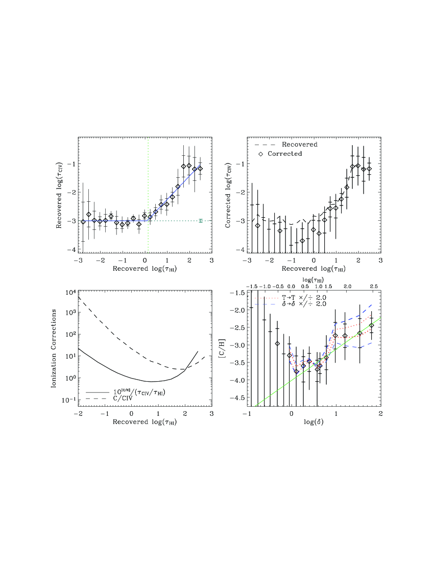
Figure 4.— Measuring the carbon abundance in Q1422+230. Data points are plotted with 1 and 2 $\sigma$ error bars. Top left: Recovered $\tau_{\rm CIV1548}$ plotted as a function of the recovered $\tau_{\rm HI1216}$. For $\tau_{\rm HI}<\tau_{c}$ (vertical dotted line) the signal is lost due to contamination, noise, and/or continuum errors and $\tau_{\rm CIV}\approx\tau_{\rm min}$ (horizontal dotted line). Top right: Corrected $\tau_{\rm CIV}$ vs. recovered $\tau_{\rm HI}$. Data points have been corrected by subtracting $\tau_{\rm min}$ from the recovered $\tau_{\rm CIV}$ plotted in the top left-hand panel and indicated here by the dashed curve. The correction affects points close to $\tau_{\rm min}$, converting the lowest points into upper limits. Bottom left: Solid and dashed curves show the ionization correction factor and the inverse of the carbon fraction, respectively. The ionization correction is insensitive to the Ly$\alpha$ optical depth in the regime where $\tau_{\rm CIV}$ is best measured. Bottom right: The carbon metallicity as a function of the overdensity (bottom axis) or $\tau_{\rm HI}$ (top axis). Data points were obtained by inserting the corrected $\tau_{\rm CIV}$, the recovered $\tau_{\rm HI}$ (i.e., the data points shown in the top right-hand panel), and the ionization correction factor (solid curve in the bottom left-hand panel) into eq.(̃6). The solid line shows the best-fit power law: $[{\rm C/H}]=-3.12_{-0.10}^{+0.09}+0.90_{-0.18}^{+0.19}(\log\delta-1.0)$. Dashed and dotted curves indicate the result of changing the density and temperature, respectively, by a factor of 2.

4. Correct the median $\tau_{\rm CIV}(\tau_{\rm HI})$. The correlation between the recovered $\tau_{\rm CIV}$ and $\tau_{\rm HI}$ flattens off at low $\tau_{\rm HI}$ where noise, continuum fitting errors, and contamination wash out the signal. In Paper I we used simulations to calibrate the difference between the true and recovered $\tau_{\rm CIV}$ and then used this information to correct the $\tau_{\rm CIV}$. Because we would like to minimize our use of the simulations and because the correction for C IV does not show any dependence on $\tau_{\rm HI}$, we choose to correct the recovered C IV optical depth using the observations themselves.

Assuming that, as is the case in the simulations (see Paper I), the asymptotic flat level $\tau_{\rm CIV}(\tau_{\rm HI}\rightarrow-\infty)$ is the median signal due to contamination, noise, and/or continuum fitting errors and that this spurious signal is independent of $\tau_{\rm HI}$, we can correct for this component to the signal by subtracting it from the data points.

The asymptotic flat level is determined as follows. We first find $\tau_{c}$, the H I optical depth below which the correlation vanishes, by fitting a power law to the data

$$\log(\tau_{\rm CIV})=\left\{\begin{array}[]{ll}A&\quad\tau_{\rm HI}<\tau_{c}\\ A+B\log(\tau_{\rm HI}/\tau_{c})&\quad\tau_{\rm HI}\geq\tau_{c}\end{array}\right.$$ (4)

Next, we define the asymptotic C IV optical depth, $\tau_{\rm min}$, as the median $\tau_{\rm CIV}$ of those pixels that have $\tau_{\rm HI}<\tau_{c}$,

$$\tau_{\rm min}\equiv{\rm median}(\tau_{\rm CIV}|\tau_{\rm HI}<\tau_{c})$$ (5)

(and similarly for other percentiles than the median). The horizontal and vertical dotted lines in the top left-hand panel of Figure 4 indicate $\tau_{\rm min}$ and $\tau_{c}$, respectively. As was the case for the data points, the error on $\tau_{\rm min}$ was computed by bootstrap resampling the spectrum. To be conservative, we add the error in $\tau_{\rm min}$ linearly (as opposed to in quadrature) to the errors on the recovered $\tau_{\rm CIV}$. Finally, for display purposes only, we fit equation (4) again to the data, but this time keeping $\tau_{\rm min}$ fixed at the value obtained before. The result is shown as the solid curve in the figure.

The corrected data points are shown in the top right-hand panel of Figure 4 and should be compared with the dashed curve in the same panel, which connects the recovered data points that were plotted in the top left-hand panel. The correction is significant only for those points that are close to $\tau_{\rm min}$. Data points with $\tau_{\rm HI}<\tau_{c}$ are effectively converted into upper limits.

5. Compute the carbon abundance as a function of density.

Assuming ionization equilibrium, which should be a very good approximation for gas photoionized by the UV background, we can compute the ionization balance of hydrogen and carbon given the density, temperature, and a model for the ionizing background radiation. As discussed in §4.3, we use CLOUDY to compute ionization balance interpolation tables as a function of redshift, density, and temperature, and we use our hydrodynamical simulation to create tables of the density and temperature as a function of redshift and H I optical depth.

To convert the optical depth measurements into metallicity estimates, we first compute the median redshift and $\tau_{\rm HI}$ of each H I bin and then use the interpolation tables to compute the corresponding density, temperature, and ionization balance. For example, the dashed curve in the bottom left panel of Figure 4 shows C/C IV, the inverse of the C IV fraction, as a function of $\tau_{\rm HI}$. The solid curve shows the ionization correction factor: $10^{[{\rm C/H}]}/(\tau_{\rm CIV}/\tau_{\rm HI})$.

Given the corrected C IV optical depth $\tau_{\rm CIV}$, the recovered H I optical depth $\tau_{\rm HI}$, and the ionization correction, we can compute the carbon metallicity:

$$[{\rm C/H}]=\log\left({\tau_{\rm CIV}(f\lambda)_{\rm HI}\over\tau_{\rm HI}(f\lambda)_{\rm CIV}}{\rm C\over CIV}{\rm HI\over H}\right)-({\rm C/H})_{\odot},$$ (6)

where $f_{i}$ and $\lambda_{i}$ are the oscillator strength and rest wavelength of transition $i$, respectively ($f_{\rm CIV}=0.1908$, $f_{\rm HI}=0.4164$, $\lambda_{\rm CIV}=1548.2041$ Å, $\lambda_{\rm HI}=1215.6701$ Å), and we use the solar abundance $({\rm C/H})_{\odot}=-3.45$ (number density relative to hydrogen; Anders & Grevesse 1989). The resulting data points are plotted in the bottom right-hand panel of Figure 4, which shows the carbon metallicity as a function of the overdensity (bottom axis) or Ly$\alpha$ optical depth (top axis).

Metals are detected over two decades in density. The median metallicity increases from a few times $10^{-4}$ around the mean density to $\sim 10^{-3}$ to $10^{-2}$ around an overdensity $\delta\sim 10^{2}$. The best-fit constant metallicity is $[{\rm C/H}]=-3.30_{-0.08}^{+0.08}$, but this fit is ruled out at high confidence ($\chi^{2}/{\rm dof}\approx 30.6/9\approx 3.4$ for the data points with $\tau_{\rm HI}>\tau_{c}$, corresponding to a probability $Q=3.5\times 10^{-4}$). The best-fit power-law metallicity is $[{\rm C/H}]=-3.12_{-0.10}^{+0.09}+0.90_{-0.18}^{+0.19}(\log\delta-1.0)$, which has $\chi^{2}/{\rm dof}\approx 3.42/8\approx 0.43$, or a probability $Q=0.91$.

The errors in this plot reflect only the errors in the corrected median $\tau_{\rm CIV}$ (top right-hand panel) and do not take uncertainties in the ionization balance into account. The dotted (dashed) curves illustrate how the metallicity changes if the temperature (density) is changed by a factor of 2. The metallicity is most sensitive to the assumed density for high $\delta$, where the ionization correction factor changes rapidly with $\tau_{\rm HI}$. Fortunately, the ionization correction is relatively insensitive to both the density and the temperature in the regime where our data is best.

5.2. The distribution of metals at a fixed density

Having measured the median carbon abundance as a function of the density, we use the simulation to check whether our measured metallicity profile can reproduce the observed optical depth statistics. The bottom set of data points in the left-panel of Figure 5 shows the observed median C IV optical depth as a function of $\tau_{\rm HI}$. The bottom solid curve shows the median $\tau_{\rm CIV}$ in the simulation (averaged over 10 spectra) for the best fit metallicity profile measured from the observations [each gas particle was given a metallicity $[{\rm C/H}]=-3.12+0.90(\log\delta-1.0)$]. Clearly, the simulation curve is a good fit of the observations ($\chi^{2}$ probability $Q=0.21$), which gives us confidence that, given a model for the UV background, our method for measuring the median carbon abundance as a function of density is robust.

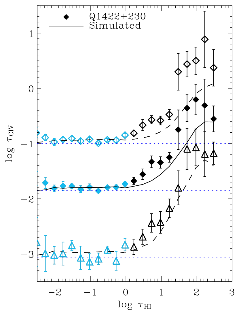
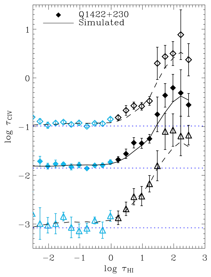
Figure 5.— Comparison of the optical depth statistics of observed and simulated spectra using the metal distribution measured from the observations. From top to bottom the three sets of data points are the 84th (open diamonds), 69th (solid diamonds) and 50th (triangles) percentiles of the recovered CIV optical depth as a function of $\tau_{\rm HI}$ for Q1422+230. For clarity, the 84th and 69th percentiles have been offset by +1.0 and +0.5 dex, respectively. The curves in the left-hand panel are for a simulation in which each particle was given the median metallicity measured from the observations, $[{\rm C/H}]=-3.12+0.90(\log\delta-1.0)$. The simulation can fit the observed median $\tau_{\rm CIV}$ ($\chi^{2}$ probability $Q=0.21$), but not the observed $\tau_{\rm CIV}(\tau_{\rm HI})$ for the other percentiles ($Q<10^{-4}$). The curves in the right-hand panel are for a simulation that has the same median metallicity, but which includes scatter. The simulation cube was divided into $10^{3}$ cubic sections, and all particles in each section were given a metallicity of $[{\rm C/H}]=-3.12+s+0.90(\log\delta-1.0)$, where $s$, which is the same for all particles in the subvolume, is drawn at random from a lognormal distribution with mean 0 and variance $\sigma=0.81~{}{\rm dex}$ as measured from the observations. The simulation provides an acceptable fit to all percentiles (from top to bottom $Q=0.33$, 0.69, and 0.90).

Although the median $\tau_{\rm CIV}$ is reproduced by the simulation, this is not the case for other percentiles. From top to bottom the sets of data points in Figure 5 correspond to the 84th, 69th, and 50th percentiles. The simulation clearly cannot reproduce the width of the observed metallicity distribution ($Q<10^{-4}$ for the higher percentiles). This indicates that the scatter in the observations is greater than can be accounted for by contamination and noise effects, both of which are present in the simulations. The scatter is also unlikely to be due to continuum fitting errors because those would result in a scatter $\sigma(\tau_{\rm CIV})$ that is independent of $\tau_{\rm HI}$, contrary to what is observed. Hence, to reproduce the observed optical depth statistics, we need to extend the method of Paper I to allow for scatter in the metallicity.

Our method to reconstruct the median metallicity can of course also be applied to other percentiles. As we will show below, for a fixed density the metallicity distribution is approximately lognormal. A lognormal distribution is parameterized by the mean $\left<\log Z\right>={\rm median}(\log Z)$ and the variance $\sigma^{2}(\log Z)$, and the fraction $f$ of pixels that have a value smaller than $x\sigma$, is given by the Gaussian integral

$$f(x)={1\over\sqrt{2\pi}}\int_{-\infty}^{x}e^{-t^{2}/2}dt.$$ (7)

For a given H I bin, we measure $\sigma$ by computing $\log Z$ for a large number of percentiles (i.e., values of $f$) corresponding to a regular grid of $x$-values, and fitting the linear function $\log Z=\sigma x$ to the data points (we use a spacing $\Delta x=0.25$ and require a minimum of four data points). The procedure is illustrated in Figure 6, which shows the measured metallicity as a function of $x$ for three different densities. The data appear well fitted by lognormal distributions (solid curves) with $\sigma\approx 0.97$ for $\delta\approx 0.9$ ($\tau_{\rm HI}=0.95$; left-hand panel), $\sigma\approx 0.73$ for $\delta\approx 4.3$ ($\tau_{\rm HI}=16.8$; middle panel), and $\sigma\approx 0.64$ for $\delta\approx 15.7$ ($\tau_{\rm HI}=94.4$, right-hand panel). Note that we cannot get reliable errors on $\sigma$ from the fits shown in the figure because the errors on the data points are all correlated since the abscissa corresponds to a ranking.

Figure 6 demonstrates that the distribution of pixel metallicities is well described by a lognormal function over at least the range $-0.5\sigma$ to $+2\sigma$. To probe the distribution further into the low-metallicity tail we would need to reduce the noise, since the lowest percentile/$x$-value corresponds to the minimum positive $\tau_{\rm CIV}$ (the rest of the pixels have a flux greater than $e^{-\tau_{\rm min}}$). To probe further into the high-metallicity tail we would need more pixels since for $N$ pixels one cannot measure a percentile greater than $(N-1)/N$ [in practice we only make use of percentiles for which $N(1-f)>5$ in order to prevent a few anomalous pixels from affecting the results].

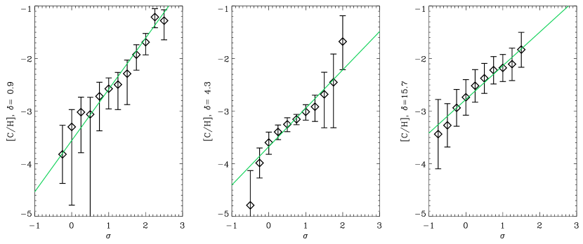
Figure 6.— Distribution of carbon metallicities for three gas overdensities: $\delta\approx 1.6$ (left), $\delta\approx 5.4$ (middle), and $\delta\approx 19.4$ (right). For each density (i.e., HI bin) the CIV pixels were ranked according to $\tau_{\rm CIV}$ and a number of percentiles were computed. The metallicity corresponding to each percentile was computed as described for the median in §5.1. The missing percentiles correspond to negative optical depths (i.e., the normalized flux is greater than unity). The curves are lognormal fits to the data points. The best-fit slopes are $\sigma([{\rm C}/{\rm H}])=0.97$, 0.73, and 0.64 for the left, middle, and right panels, respectively.

The right-hand panel of Figure 5 compares the observed percentiles with a simulation that uses a lognormal metallicity distribution, with the same median metallicity as a function of density as before and with a constant scatter of $\sigma([{\rm C}/{\rm H}])=0.81~{}{\rm dex}$ (the median value of the scatter measured in the observations for the different densities) on a comoving scale of $1.2~{}h^{-1}~{}{\rm Mpc}$. Contrary to the simulation without scatter (left-hand panel), this simulation is consistent with all the observed percentiles ($\chi^{2}$ probability $Q=0.33$, 0.69, and 0.90). To estimate the error in $\sigma([{\rm C}/{\rm H}])$ we compared the observed percentiles with those computed from simulated spectra using varying amounts of scatter in the metallicity. We find that values of $\sigma([{\rm C}/{\rm H}])=0.81\pm 0.25$ are acceptable.

Unlike the median metallicity, the scatter is independent of the assumed spectral shape of the UV background radiation. This is because the ionization correction consists of multiplying the observed optical depth ratio $\tau_{\rm CIV}/\tau_{\rm HI}$ with a factor that is independent of $\tau_{\rm CIV}$: $[{\rm C}/{\rm H}]=\log(\tau_{\rm CIV}/\tau_{\rm HI})+X$, where $X$ is the log of the ionization correction factor (see eq. [6]) which depends only on $\tau_{\rm HI}$. Hence, if $\log(\tau_{\rm CIV}/\tau_{\rm HI})$ is distributed lognormally with mean $\mu$ and variance $\sigma^{2}$, then $[{\rm C}/{\rm H}]$ is also distributed lognormally with variance $\sigma^{2}$, but with mean $\mu+X$. Note, however, that we have assumed the UV background to be uniform. If there are large fluctuations in the UV radiation at a fixed H I optical depth, then the true scatter in the metallicity could be smaller.

Having found that the metallicity distribution is well fitted by a lognormal function, we can estimate the mean metallicity as follows

$$\log\left<Z\right> = \log\left({1\over\sqrt{2\pi}\sigma}\int_{-\infty}^{+\infty}Ze^{-\left(\log Z-\left<\log Z\right>\right)^{2}/2\sigma^{2}}d\log Z\right)$$ (8)

$$= \left<\log Z\right>+{\ln 10\over 2}\sigma^{2}\approx\left<\log Z\right>+1.15\sigma^{2},$$ (9)

where $\left<\log Z\right>={\rm median}(\log Z)$ and $\sigma$ are obtained as explained above. For Q1422+230 this gives a mean metallicity of $\log\left<Z\right>\approx-2.36\pm 0.48$ at $\delta=10$.

Unlike estimates based on the mean C IV optical depth, this estimate of the mean metallicity is based on a fit to the full metallicity distribution and is thus relatively insensitive to anomalous pixels. On the other hand, since we have only a finite number of pixels, this estimate of the mean does implicitly assume that the metallicity distribution remains lognormal beyond where we can actually measure it. While the mean metallicity is insensitive to the shape of the low-metallicity tail of the distribution, the contribution of the unmeasured high-metallicity tail to the mean metallicity depends strongly on the variance. For example, cutting of the distribution at $+2\sigma$ reduces the mean by factors of 2.6 and 1.2 for $\sigma=1.0$ and 0.5 dex, respectively. For Q1422+230 we find $\sigma\approx 0.8$, which is small enough for the mean to be fairly insensitive to the unmeasured high-metallicity tail.

5.3. Summary of results for Q1422+230

Using model QG for the UV background and the $\delta(\tau_{\rm HI},z)$ and $T(\tau_{\rm HI},z)$ relations obtained from the simulations, we have found the following from analyzing the statistics of $\tau_{\rm CIV}(\tau_{\rm HI})$ in Q1422+230:

1. The observed median optical depths are inconsistent with a constant metallicity. The observations are well fitted by a median carbon abundance that is a power law of the overdensity: $[{\rm C/H}]=-3.12_{-0.10}^{+0.09}+0.90_{-0.18}^{+0.19}(\log\delta-1.0)$.

2. The distribution of $\tau_{\rm CIV}$ at fixed $\tau_{\rm HI}$ is inconsistent with a metallicity that depends only on density. The observations are well fitted by a lognormal metallicity distribution with a scatter of $0.81\pm 0.25$ dex and a median that varies as above.

6. The CIII/CIV ratio

We compute the ionization corrections as a function of the H I optical depth and redshift using interpolation tables created from the simulation. Because the simulation reproduces the observed evolution of the mean absorption (Fig. 1) and the temperature of the gas responsible for the low-column density Ly$\alpha$ lines (Schaye et al. 2000b), we are confident that the ionization balance of the gas responsible for the H I absorption is on average well determined. However, it is possible in principle that the C IV and H I absorption at a given redshift is dominated by different gas parcels. For example, Theuns et al. (2002b) predict that many of the metals produced by dwarf galaxies reside in hot gas bubbles that do not contribute significantly to the H I absorption. In their simulation most of the carbon has $T\sim 10^{6}~{}{\rm K}$ and is too highly ionized to give rise to C IV absorption. In this scenario the observed C IV absorption arises in the low-temperature tail of the carbon temperature distribution.

Although the ionization corrections are insensitive to small changes in the temperature (see Fig. 4), they could be considerably in error if the temperature were high enough for collisional ionization to be important ($T\gtrsim 10^{5}~{}{\rm K}$ for C IV). Furthermore, such a high temperature would change the relation between $\tau_{\rm HI}$ and $\delta$, causing us to underestimate the density corresponding to a given H I bin.

Figure 7.— Contour plot of $\log(\tau_{\rm CIII}/\tau_{\rm CIV})$ in the density-temperature plane. Solid and dashed contours are for the $z=3$ QG and Q UV backgrounds, respectively. For each density there is a critical temperature below which the CIII/CIV ratio is nearly constant and above which it decreases rapidly. For the densities of interest here ($n_{\rm H}\sim 10^{-5}$ to $10^{-3}$), the ratio varies from 0.1 to 10.

Fortunately, there is a way to constrain the temperature of the gas responsible for the carbon absorption by comparing the strengths of the C III ($\lambda 977$) and C IV ($\lambda\lambda 1548,1551$) transitions. Figure 7 shows a contour plot of the predicted $\log\tau_{\rm CIII}/\tau_{\rm CIV}$ in the density-temperature plane. The solid (dashed) contours are for the $z=3$ QG (Q) model of the UV background radiation. From the figure it can be seen that a measurement of the C III/C IV ratio yields an upper limit on the temperature independent of the density and the UV background.

The left-hand panel of Figure 8 shows the median C III optical depth as a function of $\tau_{\rm CIV}$ for Q1422+230. The C IV optical depths were recovered as described in §5.1, while the C III optical depths were recovered as described in Paper I for O VI, i.e., contaminating higher order Lyman lines were removed. Absorption by C III is clearly detected over 1.5 decades in $\tau_{\rm CIV}$. For $\log\tau_{\rm CIV}<-1.7$ the apparent C III optical depth is constant, indicating that for these low C IV optical depths the true $\tau_{\rm CIII}$ is smaller than the spurious signal resulting from contamination by other absorption lines, noise, and continuum fitting errors.

Note that $\log\tau_{\rm CIV}=-1.7$ corresponds to a typical H I optical depth of a few tens (see Fig. 4). Although there is considerable scatter in the $\tau_{\rm CIV}$ corresponding to a fixed $\tau_{\rm HI}$, this does suggest that we are detecting C III mostly in gas with density $\delta\gtrsim 10$. Indeed, the correlation between $\tau_{\rm CIII}$ and $\tau_{\rm HI}$ (not plotted) is detectable only for $\log\tau_{\rm HI}>1$.

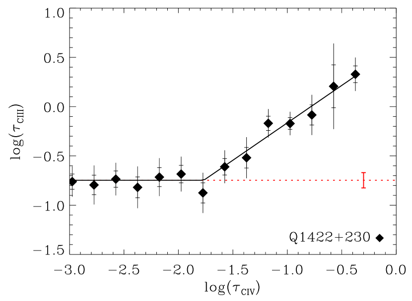
Figure 8.— $\tau_{\rm CIII}$ as a function of $\tau_{\rm CIV}$ for Q1422+230. Data points are plotted with 1 and $2\sigma$ error bars. Left: Median recovered $\tau_{\rm CIII}$ of pixels binned as a function of recovered $\tau_{\rm CIV}$. CIII is detected down to $\log\tau_{\rm CIV}\approx-1.7$. Right: The $\tau_{\rm CIII}/\tau_{\rm CIV}$ ratio is plotted as a function of $\tau_{\rm CIV}$. The median $\tau_{\rm CIII}$ were corrected for noise, contamination, etc., as described for CIV in §5.1 (step 4). The ratio $\tau_{\rm CIII}/\tau_{\rm CIV}$ is much higher than it would be if the temperature were higher than $10^{5}~{}{\rm K}$ (see Fig. 7).

We can see from Figure 7 that if the carbon were purely photoionized ($T\ll 10^{5}~{}{\rm K}$), we would expect $\tau_{\rm CIII}/\tau_{\rm CIV}$ values between 1 and 10 at $z\approx 3$ and $\delta\gtrsim 10$. The right-hand panel of Figure 8 shows the log of the ratio $\tau_{\rm CIII}/\tau_{\rm CIV}$ as a function of $\tau_{\rm CIV}$, where the $\tau_{\rm CIII}$ are the median values plotted in the left-hand panel but after subtraction of $\tau_{\rm min}$ (horizontal dashed line). The flat level $\tau_{\rm min}$ was determined in the same way as we did for $\tau_{\rm CIV}(\tau_{\rm HI})$ in §5.1 (step 4). Percentiles other than the median (not plotted) give nearly identical $\tau_{\rm CIII}/\tau_{\rm CIV}$ ratios (after subtraction of the corresponding $\tau_{\rm min}$ percentiles), indicating that this ratio is rather uniform. For $\log\tau_{\rm CIV}\gtrsim-1.5$ we detect C III and $\log\tau_{\rm CIII}/\tau_{\rm CIV}\sim 0.5$, as expected for photoionized gas at this redshift. Crucially, optical depth ratios typical for collisionally ionized C IV ($T>10^{5}~{}{\rm K}$) are ruled out by the data. Hence, the temperature of the gas responsible for the carbon absorption is smaller than $10^{5}~{}{\rm K}$, at least for densities $\delta\gtrsim 10$. This provides an important constraint for theories of the enrichment of the IGM through galactic winds and gives us confidence that our assumption that photoionization dominates is reasonable.

We have computed the C III/C IV ratio for all quasars in our sample that cover the C III region. The results are summarized in Figure 9, in which $\tau_{\rm CIII}/\tau_{\rm CIV}$, averaged over $\tau_{\rm CIV}$, is plotted as a function of redshift. While this plot uses the median $\tau_{\rm CIII}$, the other percentiles give nearly identical results. For all QSOs the ratio is in the range expected for photoionized gas with $n_{\rm H}\sim 10^{-4}~{}{\rm cm}^{-3}$ and $T<10^{5}~{}{\rm K}$. The solid line shows the best linear least absolute deviation fit to the simulated versions of all the quasar spectra, using the metallicity distributions measured from the observed spectra and the QG background. The dashed line shows a similar fit for the Q background. Overall, the simulations agree well with the observations, although they may slightly underpredict the C III/C IV ratios for $z>3$. The QG background seems to fit the data slightly better than model Q, but the difference is too small to be significant. In the simulation the small decrease in the C III/C IV ratio with time is caused both by the decrease in the typical density of C IV absorbers due to the expansion of the universe and by the hardening of the UV background radiation.

Thus, the observed C III/C IV ratios are in the range expected for photoionized gas, but are inconsistent with scenarios in which a large fraction of the C IV absorption takes place in gas with temperatures $T\gtrsim 10^{5}~{}{\rm K}$.

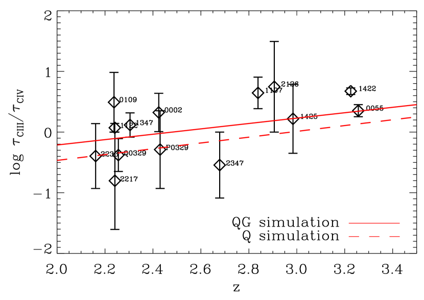
Figure 9.— The ratio $\tau_{\rm CIII}/\tau_{\rm CIV}$ is plotted as a function of redshift for all $z_{\rm em}<4$ QSOs for which CIII is covered (we do not detect CIII for QSOs above this redshift). For each QSO the median $\tau_{\rm CIII}$ were corrected for contamination, noise, etc., using the method described in §5.1 and the $\tau_{\rm CIII}/\tau_{\rm CIV}$ ratio was averaged over all bins with $\tau_{\rm CIV}>\tau_{c}$ (see §5.1 for the definition of $\tau_{c}$). The solid line shows the best linear fit to the CIII/CIV ratio measured from simulations of the same quasar spectra, which used the QG UV background and the metallicity distributions measured from the observations. The observed ratios agree well with the simulations, and comparison with Fig. 7 shows that they are in the range expected for photoionized gas with $n_{\rm H}\sim 10^{-4}~{}{\rm cm}^{-3}$ and $T<10^{5}~{}{\rm K}$.

7. Results for the full sample

In §5 we showed results for Q1422+230 to illustrate our method for measuring the distribution of carbon as a function of the gas density. In this section we will present the results from the complete sample of quasars. The results from the individual quasars are given in Appendix A.

All abundances are by number relative to the total hydrogen density, in units of the solar abundance [$({\rm C/H})_{\odot}=-3.45$; Anders & Grevesse 1989].

Our goal is to measure the carbon abundance as a function of density and redshift. For a lognormal distribution, which we found to provide a good fit to the data (see §5.2), the distribution is determined by two parameters: the mean $\left<[{\rm C}/{\rm H}]\right>={\rm median}([{\rm C}/{\rm H}])$ and the standard deviation $\sigma([{\rm C}/{\rm H}])$ (which we will often refer to as the scatter). Thus, we can characterize the full distribution of carbon by fitting functions of the two variables $\delta$ and $z$ to all the data points for $\left<[{\rm C}/{\rm H}]\right>$ and $\sigma([{\rm C}/{\rm H}])$ obtained from the individual quasars (see Fig. 1). But before doing so, it is instructive to bin the data in one variable and plot it against the other.

Figure 10 shows the median metallicity versus redshift for five different density bins of width 0.5 dex, centered about densities increasing from $\log\delta=-0.25$ (top panel) to $\log\delta=1.75$ (bottom right-hand panel). To facilitate comparison with Figure 1 we have plotted only one data point per quasar, obtained by fitting a constant metallicity to all the data points of the quasar that fall in the given density bin. The points have been labeled with the first four digits of the quasar name. The light data points have $1\sigma$ lower limits that extend to minus infinity. The solid lines in each panel show the least-squares fits to the original data points (i.e., the ones from Fig. 1, not the plotted rebinned data points) and the dotted curves indicate the $1\sigma$ confidence limits. The errors on all fits were determined by bootstrap resampling the quasars. Computing the errors using the $\chi^{2}$ surface gives similar results, although the $\chi^{2}$ errors tend to be somewhat larger (smaller) than the bootstrap errors if the $\chi^{2}$ per degree of freedom is smaller (greater) than unity. The reduced $\chi^{2}$ are somewhat small, particularly at low overdensities, indicating that we have overestimated the errors. This is not unexpected as we have used conservative estimates of the errors on data points for which the correction of the “noise” component is significant (i.e., $\tau_{\rm CIV}\approx\tau_{\rm min}$; see §5.1).

The first panel reveals that we have detected metals in underdense gas: $[{\rm C}/{\rm H}]\approx-3.6$ at $\log\delta=-0.25$, with a 2$\sigma$ lower limit of -4.12. We find that $[{\rm C}/{\rm H}]>-5$ at the $2.4\sigma$ level (99.2% confidence). For percentiles higher than the 50th (i.e., the median) the detection is even more significant. For example, for the 69th percentile we find $[{\rm C}/{\rm H}]>-5$ at the $3.4\sigma$ level. Hence, barring errors in our estimate of the density contrast, there is no question that a large fraction of underdense gas has been enriched.

At the $1\sigma$ level all bins are consistent with no evolution. The constraints are strongest for the bin $\log\delta=0.5-1.0$, in which the maximum allowed increase in the median metallicity per unit redshift is 0.14 dex at the $1\sigma$ level and 0.25 dex at the $2\sigma$ level. Comparing the metallicity at $z=3$ for the different overdensity bins, we see that the metallicity increases with overdensity from $[{\rm C}/{\rm H}]\approx-3.6$ at $\log\delta\approx-0.25$ to $[{\rm C}/{\rm H}]\approx-2.6$ at $\log\delta\approx 1.75$. This trend may be more easily analyzed using the next figure.

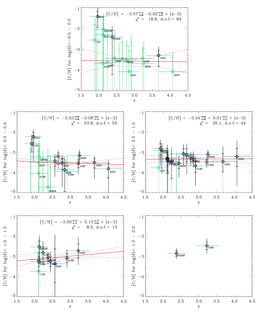
Figure 10.— Median metallicity as a function of redshift for different overdensity cuts. From the top left to the bottom right, panels correspond to the following density bins: $\log\delta=-0.5-0.0$, $0.0-0.5$, $0.5-1.0$, $1.0-1.5$, and $1.5-2.0$. One data point per QSO is plotted, labeled with the first four digits of the QSO name. Horizontal error bars indicate redshift ranges, vertical error bars indicate 1 and 2$\sigma$ errors. Light-colored data points have a lower 1$\sigma$ error of $-\infty$. For each QSO and density bin the plotted data point was obtained by fitting a constant metallicity through all the HI bins of that QSO spectrum (plotted in Fig. 1) that fall in the density bin. This rebinning was done only for visualization purposes, facilitating direct comparison with Fig. 1. The least-squares fits, shown as the solid lines, were obtained by fitting all data points (i.e., HI bins) from Fig. 1. The errors on the parameters of the fit were determined by bootstrap resampling the quasars. Dotted curves indicate the 1$\sigma$ confidence limits.

Figure 11 shows the median metallicity as a function of overdensity for three different redshift bins of width $\Delta z=1.0$ centered on $z=2$, 3, and 4. The data points were taken directly from Figure 1. As in the previous figure, light-colored data points have $1\sigma$ lower limits of $-\infty$. Note that many of the light-colored error bars correspond to data points that fall below the plotted range (some at $-\infty$). Note that the data are not uniformly distributed in these redshift bins: the median redshifts of the data points in the three bins are $z\approx 2.12$, 2.84, and 4.07. Note also that the last bin contains only two quasars: Q1055+461 and Q2237-061.

The three redshift bins give similar results, confirming that there is little evidence for evolution. We do, however, have a very significant detection of a positive gradient of metallicity with overdensity in the $z=2$ and $z=3$ bins (as seen also in the analysis of Q1422+230 in §5.1). The median metallicity increases from $[{\rm C}/{\rm H}]\approx-4$ at $\log\delta=-0.5$ to $[{\rm C}/{\rm H}]\approx-3$ at $\log\delta=1.0$. The best-fit power law index $\alpha\equiv d[{\rm C}/{\rm H}]/d\log\delta$ is $0.68_{-0.18}^{+0.10}$ for $z=2$ and $0.72_{-0.16}^{+0.07}$ for $z=3$.

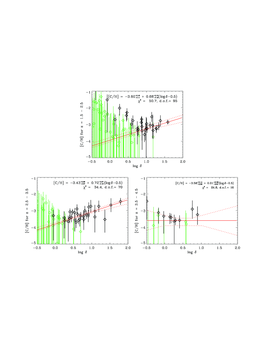
Figure 11.— Median metallicity vs. overdensity $\delta$ for different redshift bins. From the top left to the bottom right panels correspond to the following redshift ranges: $z=1.5-2.5$, $2.5-3.5$, and $3.5-4.5$. Data points with $1\sigma$ errors were taken from Fig. 1. Light-colored data points have a lower 1$\sigma$ error of $-\infty$. Solid lines indicate least-squares fits to the data points. Dotted curves indicate the $1\sigma$ confidence limits, which were computed by bootstrap resampling the quasars (for the $z=4$ bin, which contains only two quasars, we resampled the data points).

In addition to measuring $\alpha$ from the combined quasar data, we can also combine the $\alpha$ values measured in each quasar individually, which can all be read off from Figure 1. A linear least-squares fit to the data gives $\alpha=0.71_{-0.17}^{+0.10}+0.56_{-0.46}^{+0.31}\times(z-3)$ (where the errors were again computed by bootstrap resampling the quasars). As expected, the two methods of measuring the gradient of the metallicity with density give very similar results.

Let us now turn to the width of the lognormal fit to the metallicity distribution. Figure 12 shows $\sigma([{\rm C}/{\rm H}])$ versus $\delta$ (left-hand panel) and versus $z$ (right-hand panel). The data points correspond directly to the points connected by the dashed lines in Figure 1. As discussed in §5.2, our method for computing $\sigma([{\rm C}/{\rm H}])$ relies on fitting different percentiles of $\tau_{\rm CIV}$ for a fixed $\tau_{\rm HI}$, and because the percentiles are correlated, the derived error bars on $\sigma([{\rm C}/{\rm H}])$ may not be robust. However, the relative errors among the different points should still be reliable and hence the least-squares fits to the data points — shown as the solid lines in Figure 12 — should be accurate. The errors on the fits were computed by bootstrap resampling the quasars and should therefore also be robust estimates of the statistical errors. Note, however, that the fact that the measurements of the scatter are mostly one-sided (the low-metallicity tail is undetected), could result in somewhat larger systematic errors.

We find a significant ($>2\sigma$) decrease in the scatter with overdensity: $\sigma([{\rm C}/{\rm H}])=0.76_{-0.04}^{+0.03}-0.24_{-0.07}^{+0.08}(\log\delta-0.5)$. There is a hint of evolution in the data: the best-fit scatter decreases by about $0.14$ dex from $z=4$ to 2, but the a constant value is acceptable at about the $1.2\sigma$ level.

The anticorrelation of $\sigma([{\rm C}/{\rm H}])$ with $\log\delta$ is somewhat difficult to see by eye, because the trend is not large compared with the scatter between the data points. There are, however, enough points to detect weak anticorrelations. The Spearman rank-order correlation coefficient is -0.24, indicating that the anticorrelation exists at 97% confidence. Note that this test is based on a ranking of the data points and does not make use of the errors.

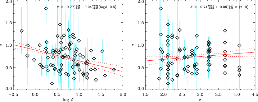
Figure 12.— Standard deviation of the lognormal metallicity distribution as a function of overdensity (left) and redshift (right). Data points with $1\sigma$ errors correspond to the HI bins shown in Fig. 1. The relative sizes of the errors are reliable, but the absolute sizes are not. Solid lines are least-squares fits to the data points. Dotted curves indicate the $1\sigma$ confidence limits, which were computed by bootstrap resampling the quasars.

We can summarize all of our data by fitting functions of redshift and overdensity to the median metallicity and the (lognormal) scatter, using all the $\log\delta>-0.5$ data points shown in Figure 1. The function

$$[{\rm C}/{\rm H}] = -3.47_{-0.06}^{+0.07}+0.08_{-0.10}^{+0.09}\times(z-3)$$ (10)

$$+0.65_{-0.14}^{+0.10}\times(\log\delta-0.5)$$

provides a very good fit to the data: $\chi^{2}=114.1$ for 184 degrees of freedom. As for the projection fits, the reduced $\chi^{2}$ is low because we overestimated the errors for the data points with $\tau_{\rm CIV}\approx\tau_{c}$, i.e., points for which C IV is barely detected (see §5.1). Excluding all data points with $\tau_{\rm HI}<\tau_{c}$ does not change the fit (the differences are smaller than the statistical errors), but does result in a much more reasonable reduced $\chi^{2}$ of 0.89.

To test whether there is evidence for density-dependent evolution or, equivalently, a redshift-dependent gradient with density, we have also fitted a function including a $(z-3)(\log\delta-0.5)$ term to the data. The best-fit coefficient of the cross term is consistent with zero at the $\approx 0.8\sigma$ level, and including it improves the quality of the fit only slightly, to $\chi^{2}=112.5$ for 183 dof.

Fitting a three-parameter surface to the scatter in the lognormal distribution yields

$$\sigma([{\rm C}/{\rm H}]) = 0.76_{-0.08}^{+0.05}+0.02_{-0.12}^{+0.08}\times(z-3)$$ (11)

$$-0.23_{-0.07}^{+0.09}\times(\log\delta-0.5).$$

As was the case for the median, using the four-parameter function does not improve the fit and yields no evidence for a nonzero coefficient of the $(z-3)(\log\delta-0.5)$ term.

The best-fit parameters for all the surface fits are listed together with their 1 and $2\sigma$ errors in Tables 2 and 3. Note that all these fits are based on data in the range $\log\delta=-0.5-1.8$ ($\log\delta=-0.5-0.9$ for $z>3.5$), $z=1.8-4.1$ ($z=2.1-3.3$ for $\log\delta>1$) and that extrapolations outside this range of parameter space could be inaccurate.

Table 2Fits for $[{\rm C}/{\rm H}]=\alpha+\beta(z-3)+\gamma(\log\delta-0.5)$

Model	$\alpha_{-1\sigma,\,2\sigma}^{+1\sigma,\,2\sigma}$	$\beta_{-1\sigma,\,2\sigma}^{+1\sigma,\,2\sigma}$	$\gamma_{-1\sigma,\,2\sigma}^{+1\sigma,\,2\sigma}$	$\chi^{2},{\rm d.o.f.}$
QG	$-3.47_{-0.06,\,0.12}^{+0.07,\,0.13}$	$+0.08_{-0.10,\,0.20}^{+0.09,\,0.19}$	$+0.65_{-0.14,\,0.27}^{+0.10,\,0.18}$	114.1, 184
Q	$-2.91_{-0.07,\,0.13}^{+0.07,\,0.13}$	$-0.06_{-0.09,\,0.19}^{+0.09,\,0.21}$	$+0.17_{-0.08,\,0.21}^{+0.08,\,0.15}$	113.8, 184
QGS3.2	$-3.78_{-0.09,\,0.16}^{+0.14,\,0.21}$	$-0.12_{-0.12,\,0.22}^{+0.06,\,0.13}$	$+0.93_{-0.32,\,0.47}^{+0.18,\,0.28}$	124.2, 184
QGS	$-4.14_{-0.05,\,0.11}^{+0.06,\,0.11}$	$+0.54_{-0.07,\,0.16}^{+0.10,\,0.21}$	$+1.31_{-0.07,\,0.18}^{+0.07,\,0.17}$	114.2, 184

Table 3Fits for $\sigma=\alpha+\beta(z-3)+\gamma(\log\delta-0.5)$

Model	$\alpha_{-1\sigma,\,2\sigma}^{+1\sigma,\,2\sigma}$	$\beta_{-1\sigma,\,2\sigma}^{+1\sigma,\,2\sigma}$	$\gamma_{-1\sigma,\,2\sigma}^{+1\sigma,\,2\sigma}$
QG	$+0.76_{-0.08,\,0.16}^{+0.05,\,0.09}$	$+0.02_{-0.12,\,0.22}^{+0.08,\,0.17}$	$-0.23_{-0.07,\,0.15}^{+0.09,\,0.21}$
Q	As for QG
QGS3.2	As for QG
QGS	As for QG

The surface fits confirm the picture suggested by the projection plots. There is very little room for evolution, but there is strong evidence for both an increase in the median metallicity and a decrease in the lognormal scatter with overdensity.

7.1. Varying the UV background

All ionization corrections were computed as discussed in §4.3, using model QG (Haardt & Madau 2001) for the UV/X-ray background from galaxies and quasars (see §4.2), rescaled to match the evolution of the mean Ly$\alpha$ absorption as measured from our sample of observations (see §3). Since the spectral shape of the UV background is not well constrained, it is important to investigate what effect changes in the spectrum have on the derived metallicities.

In particular, since photons with energies greater than 4 ryd can ionize C IV but not C III, the ionization corrections can be sensitive to the break at the He II Lyman limit, which is much greater if the background is dominated by stars as opposed to quasars, and can also be very large if He II is not fully reionized. As Figure 3 shows, for gas with densities $n_{\rm H}\lesssim 10^{-5}~{}{\rm cm}^{-3}$ the $z=3$ ionization correction is much larger for model Q — which includes only contributions from quasars — than for model QG. Thus, as expected, for low gas densities the derived metallicity is sensitive to the hardness of the UV background radiation, with harder spectra yielding higher metallicities.

To investigate how sensitive the metallicities are to changes in the UV radiation field, we have recomputed the surface fit $[{\rm C}/{\rm H}](\delta,z)$ (eq. [10]) using the two additional models for the UV background radiation described in §4.2. Model Q (Haardt & Madau 2001) is an updated version of the Haardt & Madau (1996) model for the background radiation from quasars only. Model QGS is identical to model QG, except that above 4 ryd the flux has been decreased by a factor of 10. The results are listed in Table 2.

Model QGS is much softer than model QG and therefore gives lower metallicities and a much stronger gradient with overdensity. In addition, the metallicity is everywhere decreasing with time, clearly an unphysical result. We get the same unphysical trend if we decrease the flux above 4 ryd by only a factor of 3 instead of a factor of 10 as in QGS. Although using model QGS at all redshifts results in a metallicity evolution that does not make physical sense, QGS could be a reasonable model for the UV background at $z\sim 4$ if He II was reionized late. We have therefore tested model QGS3.2, which is identical to model QG for $z<3.2$ and identical to model QGS for $z>3.2$. This transition redshift was chosen because various lines of evidence suggest that He II reionization was incomplete at earlier times (e.g., Songaila 1998; Schaye et al. 2000b; Heap et al. 2000; Theuns et al. 2002a).

Figure 13 shows the two projections of the three-parameter surface fits (listed in Table 2) for models QG, Q, and QGS3.2. The left-hand panel shows the median metallicity versus $\log\delta$ for $z=3$, while the right-hand panel plots the median metallicity versus $z$ for $\log\delta=0.5$. Although these plots cannot shed light on density-dependent evolution, they do illustrate the key differences between the various UV backgrounds.

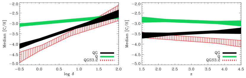
Figure 13.— Visualization of the fits to the median metallicity as a function of overdensity and redshift for $z=3$ (left-hand panel) and $\log\delta=0.5$ (right-hand panel) for our fiducial UV background model QG, as well as for models Q and QGS3.2. The shaded regions enclose the $1\sigma$ confidence contours for the three-parameter surface fits listed in Table 2. Harder UV backgrounds yield higher metallicities for $\delta<10$. Strong evolution is ruled out for all models.

As for model QG, model Q gives no evidence for evolution. However, for model Q the results do differ from our fiducial model in other ways. Model Q yields much higher metallicities for $\log\delta<1$ and gives a much smaller gradient of the median metallicity with density. In the next section we will show that this small gradient, combined with the observed decrease in the scatter with density, results in a mean metallicity that decreases significantly with increasing density, probably an unphysical result. Note that model Q also does not fare as well as model QG in fitting the observed C III/C IV ratios (see §6).

Model QGS3.2 yields a significantly lower metallicity for $z>3.2$ than our fiducial QG model. As a result, there is evidence for (weak) evolution ($d[{\rm C}/{\rm H}]/dz=-0.12_{-0.12}^{+0.06}$). Because many of our low-density detections have high redshifts, the gradient with overdensity is even stronger than for model QG. Since it is only the high-redshift data that are responsible for the larger gradient, there is evidence for density-dependent evolution, including a cross term in the fit improves it by $\Delta\chi^{2}=9$ relative to the three-parameter fit.

Although uncertainties in the UV background are important for estimates of the median metallicity, this is not the case for our measurements of the lognormal scatter, which are independent of the assumed UV background (see s5.2). Our finding that the metallicity distribution is lognormal and our measurements of the scatter in this distribution are therefore much less model-dependent than our measurements of the median metallicity. They are, however, still not completely model-independent because we have assumed that the UV radiation is constant for fixed $\tau_{\rm HI}$. If there were significant scatter in the UV radiation field corresponding to a fixed overdensity, then this would generate scatter in the $\tau_{\rm CIV}$ distribution, leading us to overestimate the width of the metallicity distribution.

8. Discussion

8.1. Summary of measurements

We have measured the distribution of carbon as a function of overdensity and redshift using data in the range $\log\delta=-0.5-1.8$ and $z=1.8-4.1$. For a fixed overdensity and redshift the metallicity distribution is close to lognormal, at least from about $-0.5$ to $+2\sigma$. We measure a lognormal scatter $\sigma([{\rm C}/{\rm H}])=0.76_{-0.08}^{+0.05}+0.02_{-0.12}^{+0.08}(z-3)-0.23_{-0.07}^{+0.09}(\log\delta-0.5)$. Thus, we find no evidence for evolution, but we do find a significant decrease in the scatter with overdensity. The measurements of the scatter are independent of the spectral shape of the UV background radiation.

Unlike the scatter, the median metallicity does depend on the model for the UV background, although it is insensitive to the spectral shape for $\delta\gtrsim 10$. For our fiducial model QG, which includes contributions from both galaxies and quasars (see Haardt & Madau 2001), we find $[{\rm C}/{\rm H}]=-3.47_{-0.06}^{+0.07}+0.08_{-0.10}^{+0.09}(z-3)+0.65_{-0.14}^{+0.10}(\log\delta-0.5)$, i.e., no evidence for evolution, but a strong gradient with overdensity.

Harder UV backgrounds yield higher metallicities at low overdensities. Model Q, which includes only UV radiation from quasars, gives a median metallicity higher by about 0.6 dex for $\log\delta=0.5$, a much weaker gradient with overdensity ($d[{\rm C}/{\rm H}]/d\log\delta=0.17_{-0.08}^{+0.08}$), but again no evidence for evolution. As we will discuss below, this UV background is probably too hard since it yields a mean metallicity that decreases with overdensity. Note that measurements of $N_{\rm HeII}/N_{\rm HI}$ also imply that the true UV background is softer than model Q (Heap et al. 2000; Kriss et al. 2001). Making the UV background too soft also gives unphysical results: model QGS, which has a 10 times smaller flux above 4 ryd than model QG, yields a metallicity that strongly decreases with time for all overdensities. We find the same unphysical trend if we decrease the flux above 4 ryd by a factor of 3 instead of 10.

Hence, it appears that the metal distribution (median and scatter) evolves very little from $z=4$ to $z=2$, which suggests that most of the enrichment of the low-density IGM took place at higher redshifts. There is, however, a caveat: we do find (weak) evolution in the median metallicity if we make the UV background much softer at high redshift (or much harder at low redshift). For example, model QGS3.2, which has a 10 times smaller flux above 4 ryd for $z>3.2$ (as may be appropriate if He II had not yet reionized by that time), gives $d[{\rm C}/{\rm H}]/dz=-0.12_{-0.12}^{+0.06}$ for $\log\delta=0.5$ and stronger evolution for lower overdensities.

Note that even if the enrichment of the IGM was completed at $z\gg 4$, one would still expect some evolution in the gradient of metallicity with overdensity, unless the initial gradient was zero. Because gravity tends to increase density contrasts, any initial gradient of metallicity with overdensity should become weaker with time. In fact, our measurements favor a small increase in the gradient with redshift: for model QG the coefficient of the $(z-3)(\log\delta-0.5)$ term in our four-parameter surface fit is $0.23_{-0.28}^{+0.15}$. Although a detailed comparison with models for the enrichment of the IGM is beyond the scope of this paper, we note that the simulations we have performed show that the expected “passive” evolution in the gradient of the metallicity with overdensity from $z=4$ to $z=2$ is sufficiently small to be easily compatible with our measurements.

8.2. Mean metallicities

Having measured the median and the scatter of the lognormal distribution, we can also compute the mean (see eq. [9]). For our fiducial model we find $\log\left<Z\right>\approx-2.8$ at $\log\delta=0.5$, where $Z$ is short for $10^{[{\rm C}/{\rm H}]}$, with no evidence for evolution. At the 1$\sigma$ ($2\sigma$) level the data allow an increase of about 0.1 dex (0.3 dex) per unit redshift. For model Q, $\log\left<Z\right>$ is $\sim 0.6$ dex higher at this overdensity and, as for model QG, there is no evidence for evolution. Note that the limits on the allowed evolution of the mean metallicity are weaker than for the median metallicity because there is additional uncertainty in the redshift dependence of the lognormal scatter.

For our fiducial model the mean metallicity increases with overdensity from $\log\left<Z\right>=-2.9$ at $\delta\sim 1$ to -2.3 at $\delta\sim 10^{2}$ for $z=3$. For model Q, however, it decreases from -2.1 to -2.5 over the same density range. This negative gradient is significant at the $1\sigma$ (but not $2\sigma$) level and may imply that model Q is unphysical since models for the enrichment of the IGM generically predict positive metallicity gradients with overdensity (e.g., Cen & Ostriker 1999; Aguirre et al. 2001a, 2001b).

8.3. Global metallicities

By combining our measurements of the carbon distribution (equations [10] and [11]) with the mass-weighted probability density distribution for the gas density obtained from our hydrodynamical simulation, we can compute the contribution of the carbon that we see to the global, mass-weighted mean metallicity. For $z=3$ and $\log\delta=-0.5-2.0$ we find a cosmic carbon abundance $[{\rm C}/{\rm H}]=-2.80\pm 0.13$, with no evidence for evolution. Extrapolating our measurements to the full density range of the simulation, we find $[{\rm C}/{\rm H}]=-2.56\pm 0.16$ (the higher overdensities being responsible for the difference). For model Q all values are about 0.5 dex higher.

Relative to the critical density, our measurement of the contribution of the forest to the global carbon abundance corresponds to a global carbon density of

$$\Omega_{\rm C} = 10^{[{\rm C}/{\rm H}]+({\rm C/H})_{\odot}}m_{\rm C}{\bar{n}_{\rm H}\over\rho_{c}},$$ (12)

$$\approx 2.3\times 10^{-7}10^{[{\rm C}/{\rm H}]+2.8}\left({\Omega_{b}\over 0.045}\right),$$ (13)

where $m_{\rm C}$ is the atomic mass of carbon, $\bar{n}_{\rm H}$ is the total, comoving number density of hydrogen, and $\rho_{c}$ is the critical mass density at redshift zero.

8.4. Filling factors

The dashed curves in Figure 14 show the fraction of gas with a metallicity greater than $[{\rm C}/{\rm H}]$ as a function of $[{\rm C}/{\rm H}]$ for various overdensities. All curves are for model QG and $z=3$. The filling factors were computed using the surface fits to the median metallicity and lognormal scatter as a function of overdensity and redshift (equations [10] and [11]). Note that for metallicities below the median (i.e., filling factor 0.5), we detect C IV only for significantly overdense gas. Thus, the lognormal shape of the curves in the upper half of the plot is a result of extrapolating the shape measured for the bottom half. The thick, solid curve shows the total filling factor, i.e., the volume fraction. It was computed by combining our metallicity measurements with the volume weighted probability density distribution for the gas density in our hydrodynamical simulation at $z=3$ (using a physical smoothing scale of 75 kpc). The filling factors for $z=2$ and $z=4$ (not plotted) fall nearly on top of this curve.

Figure 14 summarizes many of our results. The intersection of the dashed curves with the filling factor 0.5 gives the median metallicity at the various overdensities. The fact that the dashed curves become steeper going from low to high overdensities (left to right) reflects our finding that the scatter decreases with overdensity. One consequence of this is that high-metallicity gas ($[{\rm C}/{\rm H}]\gg-2$) is rare. For all metallicities the filling factor increases with overdensity. For model Q, which gives a median metallicity that is nearly independent of overdensity, this is in fact not the case for high metallicities. Since a filling factor that decreases with overdensity seems implausible, this again suggests that the UV radiation is too hard in model Q.

Essentially all collapsed gas clouds ($\delta\gtrsim 10^{2}$) have a metallicity greater than $5\times 10^{-4}~{}Z_{\odot}$. Metallicities of 1 and 5 times $10^{-4}$ have been claimed to be the maximum possible metallicities for the formation of supermassive stars (Bromm et al. 2001; Schneider et al. 2002). Our results therefore indicate that by $z=4$ the formation of such stars had already come to an end. Some caution is appropriate, however, because the top parts of the dashed curves are based on extrapolations since we generally detect C IV only if the metallicity is similar or greater than the median value.

Figure 14.— Filling factor of gas with a carbon abundance greater than $[{\rm C}/{\rm H}]$ plotted as a function of $[{\rm C}/{\rm H}]$ for $z=3$ and UV background QG. Dashed curves indicate the filling factors at overdensities of, from left to right, $\log\delta=-0.5,0.0,\ldots,2.0$. The thick solid curve indicates the total filling factor, i.e., the volume fraction.

8.5. Do we see all of the carbon?

Throughout this paper we assumed that the C IV gas has a temperature $T\ll 10^{5}~{}{\rm K}$, so that collisional ionization is unimportant. Our measurements of the C III/C IV ratio strongly support this assumption for $\log\delta\gtrsim 1$, but cannot rule out high temperatures for lower density gas. However, the fact that we detect C IV generally even for H I optical depths as low as $\tau_{\rm HI}\sim 1$ implies that hot gas would need to have a substantial filling factor to invalidate the assumption that the gas that we observe is predominantly photoionized. Note that Carswell et al. (2002) and Bergeron et al. (2002) could rule out collisional ionization for many of the O VI absorbers associated with low column density H I systems on the basis of their line widths.

Gas with a temperature $T\gg 10^{5}~{}{\rm K}$ is too highly ionized to cause detectable absorption in C IV or H I and will therefore not introduce errors in our measurements of the metallicity of the warm, photoionized component. It is, however, important to note that our analysis cannot reveal carbon hidden in hot, X-ray–emitting gas, which may contain a large fraction of the intergalactic metals (Theuns et al. 2002b). The same is true for cold, self-shielded gas for which most of the carbon is neutral or singly ionized. Comparisons to models in which a significant fraction of intergalactic carbon is in gas with $T\gg 10^{5}~{}{\rm K}$ or $T\ll 10^{4}~{}{\rm K}$ must therefore be made with care.

8.6. Comparison to previous work

There have been no previous systematic attempts to measure the metal distribution in the Ly$\alpha$ forest as a function of overdensity and redshift. Previous studies using C IV pixel statistics (Cowie & Songaila 1998; Ellison et al. 1999, 2000) reported optical depth measurements consistent with our results. However, these studies used less sensitive methods, considered only the median $\tau_{\rm CIV}$, and did not attempt to correct for ionization. Published measurements of the carbon abundance have generally been based on a comparison of Voigt profile statistics of C IV lines with either a hydrodynamical simulation assuming a uniform metallicity or simple photoionization models for individual absorbers.

Both simulations (e.g., Haehnelt et al. 1996, Rauch et al. 1997; Hellsten et al. 1997; Davé et al. 1998) and simple photoionization models (e.g., Cowie et al. 1995; Songaila & Cowie 1996; Rollinde et al. 2001; Carswell et al. 2002) find that a carbon abundance of $10^{-3}$ to $10^{-2}$ solar reproduces the $z\sim 3$ observations. Rauch et al. (1997), Hellsten et al. (1997), and Davé et al. (1998) all find $[{\rm C}/{\rm H}]=-2.5$ and also report evidence for scatter of about 1.0 dex (Davé et al. 1998 find 0.5 dex). These studies used the relatively hard Haardt & Madau (1996) model for the UV background from quasars, which closely resembles our model Q. For this model we find a median metallicity at $z=3$ of $[{\rm C}/{\rm H}]=-2.91_{-0.07}^{+0.07}+0.17_{-0.08}^{+0.08}(\log\delta-0.5)$ and a lognormal scatter of $\sigma([{\rm C}/{\rm H}])=0.76_{-0.08}^{+0.05}-0.23_{-0.07}^{+0.09}(\log\delta-0.5)$, both nearly independent of redshift. However, compared with our work, the metallicity measurements of previous studies were dominated by denser gas: $\log\delta\sim 1.0-1.5$. For these densities we find a scatter of about 0.6 dex, a median metallicity $[{\rm C}/{\rm H}]\approx-2.8$, and a mean metallicity $\log\left<[{\rm C}/{\rm H}]\right>\approx-2.4$ (see eq. [9]; note that it is unclear whether we should be comparing the mean or the median when comparing with previous work). Hence, if we use a hard UV background and focus on the high density gas ($N_{\rm HI}\sim 10^{15}-10^{16}~{}{\rm cm}^{-2}$), then our results for $z=3$ agree with the metallicity measurements obtained by previous studies. However, our fiducial UV background (QG) gives a smaller metallicity, particularly at low overdensities.

Songaila (2001) measured the C IV column density distribution as a function of redshift from $z=1.5$ to$z=5.5$ and found no evidence for evolution. It is, however, important not to overinterpret this finding. To draw conclusions about the evolution of the metallicity, one must correct for ionization, and this correction is time-dependent because the universe expands and the UV background evolves.

Songaila (2001; see also Pettini et al. 2003) also computed $\Omega_{\rm CIV}$ as a function of redshift by summing all of the observed C IV systems. This provides a strict lower limit to $\Omega_{\rm C}$ because not all carbon is triply ionized and because some C IV systems may have been lost in the noise and contamination. Finite sample size is also important because the integrals of fits to the C IV column density distribution diverge at high $N_{\rm CIV}$. Songaila found $\Omega_{\rm CIV}(10^{12}~{}{\rm cm}^{-2}\leq N_{\rm CIV}\leq 10^{15}~{}{\rm cm}^{-2})\approx(3\pm 2)\times 10^{-8}$ at all redshifts. Using our measurements of the carbon distribution for model QG and the mass-weighted probability density distribution for the gas density from our hydrodynamical simulation, we find $\Omega_{\rm C}\approx(2.3\pm 0.7)\times 10^{-7}$ for $\log\delta=-0.5-2.0$, with no evidence for evolution (see §8.3). For model Q the cosmic carbon abundance is about a factor of 3 higher, again with no evidence for evolution. Thus, we find that $\Omega_{\rm C}$ is indeed much higher than $\Omega_{\rm CIV}$ measured by Songaila (2001). The large difference implies that the observed evolution of $\Omega_{\rm CIV}$ tells us very little about the evolution of $\Omega_{\rm C}$.

Nevertheless, Songaila’s measurements of $\Omega_{\rm CIV}$ provide an important consistency check. Using our measurements of the distribution of carbon, the density distribution of our hydrodynamical simulation, and our ionization correction as a function of overdensity and redshift, we can compute $\Omega_{\rm CIV}$. For $-0.5\leq\log\delta\leq 2.0$ we find $\Omega_{\rm CIV}/10^{-8}\approx 1.3\pm 0.8$, $4\pm 1$, and $8\pm 5$ for $z=2$, 3, and 4, respectively (as expected, the different UV background models give similar numbers). The values are nearly the same if we extrapolate to higher or lower overdensities, which implies that we are seeing most of the C IV. The quoted errors are estimates of the statistical errors; i.e., they are based on the errors on the parameters of the surface fits. Note that the difference between $\Omega_{\rm CIV}$ and $\Omega_{\rm C}$ decreases from $z=2$ to $z=4$. Thus, our results are in good agreement with those of Songaila (2001). Given that our calculation of $\Omega_{\rm CIV}$ relies on convolving our measured carbon distribution with the gas distribution extracted from our simulation, this is a highly nontrivial consistency check.

8.7. Uncertainties

Our method contains several steps and parameters chosen to minimize the errors in the metallicity measurements in simulated spectra. To test the robustness of our method to these choices, we have redone the surface fits after dividing each quasar spectrum in two, doubling the H I bin size, omitting our correction to the continuum fit of the C IV region, excluding all data with $\delta<1$, excluding all data with $\tau_{\rm HI}<\tau_{c}$, or excluding all H I bins containing fewer than 50 pixels and/or contributions from fewer than 10 different chunks (our fiducial values for these parameters are 25 and 5, doubling them removes many of the higher H I bins). We find that the coefficients of the various surface fits always agree within their errors with those obtained using our standard method. Thus, our results are insensitive to the details of our method and the surface fits are not determined by the highest/lowest H I bins.

Although our results are robust with respect to small changes in the methodology, there could of course still be systematic errors. The main uncertainty in the median metallicity comes undoubtedly from the uncertainties in the spectral shape of the UV background. Although the lognormal scatter is independent of the mean spectral shape, it is sensitive to fluctuations. If there were significant fluctuations in the UV background, then this would introduce scatter in the $\tau_{\rm CIV}(\tau_{\rm HI})$ relation even for a uniform metallicity, particularly at low overdensities where the ionization correction is large. If fluctuations are important, then our measurements should be interpreted as upper limits on the scatter in the metallicity.

Even for a uniform UV background there are likely to be some systematic errors in our ionization corrections. For example, our measurements of the C III/C IV ratio cannot rule out the possibility that collisional ionization is important for $\delta\ll 10$. At some level, the ionization corrections must be incorrect, since redshift-space distortions will result in multiple gas elements contributing to the absorption at a fixed redshift.

Fortunately, we can use our hydrodynamical simulation to estimate the size of these and other systematic uncertainties: we can distribute metals in our simulation according to our measurements, create synthetic versions of our observations, and then compare the simulated and observed optical depth statistics. In §5.2 we showed that our method passed this test for Q1422+230. It is important to note that interpreting the results of this test is not completely straightforward, because there is some ambiguity in the interpretation of our measurements. For example, we do not know the exact scale on which our overdensities are smoothed (probably $\sim 50-100~{}{\rm kpc}$; see §4.3), and we do not know the exact scale(s) over which we are measuring the scatter. Consequently, it is not completely clear how to distribute the metals in the simulations. Having said this, we expect the density smoothing scale to be similar to the smoothing scale of the forest — which depends on the gas density and is not very different from the resolution of our simulation — and we find that the precise scale on which the scatter is imposed is not critical provided it is greater than the smoothing scale of the forest.

We have carried out the test described above (and in more detail in §5.2) for our entire sample, distributing the metals in our simulations according to equations (10) and (11), although we neglected the small, observed decrease in the scatter with overdensity since we have no practical way of implementing such a trend in the simulation (we imposed the scatter on a scale of $1.2h^{-1}\,{\rm Mpc}$ comoving, i.e., 1/10th of the simulation box size). Averaging over 10 realizations, we find for the data points with $\tau_{\rm HI}>\tau_{c}$ a reduced $\chi^{2}$ of 1.02, 0.97, and 1.35 for the 50th, 69th, and 84th percentiles, respectively. The total number of data points included in this estimate is 92 for the 50th percentile and 95 for the other two percentiles. Hence, we have a model that can reproduce the observed optical depth statistics. It appears that any systematic errors must be small and that the ambiguities discussed above are not critical.

We also carried out the following, more stringent test. As before, we first generate a set of synthetic observations using our three-parameter fits to the data (eqs. [10] and [11], but with $d\sigma/d\log\delta=0$). Second, we measure the carbon abundance from the simulated spectra in the same way as we did for the data, and we fit the same three-parameter functions to the results. Finally, we compare the fits to the ones we started with. The differences between the fits give us estimates of the systematic errors, or rather upper limits to the systematic errors given the ambiguities in the smoothing scale discussed above. Averaging over 10 realizations we find systematic errors for the coefficients of the median metallicity (eq. [10]) of $\Delta\alpha=-0.10$ ($1.7\sigma$), $\Delta\beta=-0.20$ ($2.0\sigma$), and $\Delta\gamma=-0.14$ ($1.0\sigma$), where the numbers in brackets give the ratios of the systematic to the statistical errors. The variance between the different realizations is comparable to the statistical errors. Note that the signs of the systematic errors is such that we may have slightly overestimated the evolution (i.e., $d[{\rm C}/{\rm H}]/dz$ too negative) and underestimated the gradient with overdensity. For the coefficients of the scatter (eq. [11]) we find $\Delta\alpha=-0.11$ ($0.69\sigma$), $\Delta\beta=0.02$ ($0.25\sigma$), and $\Delta\gamma=0.01$ ($0.11\sigma$). Thus, the systematic errors are small for the scatter, but may not be insignificant for the normalization ($\alpha$) and the trend with redshift ($\beta$) of the median. No systematic errors are greater than twice the corresponding statisical errors. Although these tests give us confidence that our results are robust, they do of course not rule out the existence of other, unknown, sources of systematic errors.

8.8. Future prospects

How could our measurements be improved? Higher signal-to-noise ratios (and better continuum fits, but these are signal-to-noise limited) are required to measure the median metallicity at lower overdensities and to verify that the metal distribution remains lognormal below the median metallicity. Better coverage of the higher-order Lyman lines would enable us to increase the number of data points for $\log\delta>1$. To improve the constraints on the evolution more data at $z>3$ would be very helpful since only four out of our 19 quasar spectra have a median redshift greater than 3. For $\delta<10$ the median metallicity becomes increasingly sensitive to the softness of the UV radiation, and it will be necessary to improve the constraints on the spectral shape of the UV background to tighten the constraints.

9. Conclusions

We have measured the statistical correlation between C IV and H I absorption in a sample of 19 high resolution VLT/UVES and Keck/HIRES spectra of QSOs spanning a redshift range $\sim 1.5-4.5$. Hydrodynamical simulations (which can reproduce the observed statistics of the Ly$\alpha$ forest) link the observed H I absorption to the density and temperature of the absorbing gas. Given a model of the ionizing background radiation field, this allows us to convert the median ratio of C IV to H I pixel optical depths into a median carbon abundance $[{\rm C}/{\rm H}]$ as a function of density and redshift. In Paper I we tested this technique extensively on realistic simulated spectra, and here we have generalized the method to recover the distribution of metals from the full distribution of $\tau_{\rm CIV}$ as a function of $\tau_{\rm HI}$.

Our fiducial model for the UV background is that of Haardt & Madau (2001) — which includes contributions from both galaxies and quasars — renormalized using our measurements of the evolution of the mean Ly$\alpha$ absorption.

Our primary conclusions are as follows:

• The best-fit power-law evolution of the effective Ly$\alpha$ optical depth in the spectra of 21 quasars is $\log\tau_{\rm eff}=(-0.44\pm 0.01)+(3.57\pm 0.20)\log[(1+z)/4]$. Contamination from metal lines — which we removed before making these measurements — is significant, particularly at lower redshifts.

• C III to C IV optical depth ratios typical of collisionally ionized C IV ($T\gtrsim 10^{5}~{}{\rm K}$) are ruled out by the data, at least for overdensities $\delta\gtrsim 10$. Simulations with $T\sim 10^{4}~{}{\rm K}$ naturally reproduce the observations. The existence of very hot ($T\gg 10^{5}~{}{\rm K}$) or very cold ($T\ll 10^{4}~{}{\rm K}$) carbon cannot be ruled out as it would not give rise to significant C III or C IV absorption.

• For a fixed overdensity $\delta$ and redshift $z$ the metallicity distribution is close to lognormal, at least from about $-0.5$ to $+2\sigma$.

• Over the range $\log\delta=-0.5-1.8$ and $z=1.8-4.1$ the median carbon abundance is well fitted by the following function: $[{\rm C}/{\rm H}]=-3.47_{-0.06}^{+0.07}+0.08_{-0.10}^{+0.09}(z-3)+0.65_{-0.14}^{+0.10}(\log\delta-0.5)$. The overdensities have effectively been smoothed on the same scale as the Ly$\alpha$ forest ($\sim 50-100~{}{\rm kpc}$). From tests using simulations we find that the known systematic errors are at most twice as large as the quoted statistical errors. There is no evidence for a nonzero $(z-3)(\log\delta-0.5)$ term. Thus, we find no evidence for evolution, but strong evidence for a positive gradient with overdensity.

• Harder UV backgrounds give higher carbon abundances for $\log\delta<1$ and thus smaller gradients with overdensity. The (rescaled) Haardt & Madau (2001) quasar only UV background yields a mean metallicity that decreases with overdensity, which is probably unphysical. UV backgrounds that are much softer than our fiducial model result in a median (and mean) metallicity that strongly increases with redshift, which is also unphysical. However, a UV background that is softer only for $z>3.2$, as may be appropriate if the reionization of He II was incomplete before this time, is allowed and results in significant (but still weak) evolution in the median metallicity.

• We find a nonzero median carbon abundance for underdense gas ($\log\delta=-0.5-0.0$) at the 99.2% ($2.4\sigma$) confidence level.

• The lognormal scatter is $\sigma([{\rm C}/{\rm H}])=0.76_{-0.08}^{+0.05}+0.02_{-0.12}^{+0.08}(z-3)-0.23_{-0.07}^{+0.09}(\log\delta-0.5)$. Our measurements of the scatter are strictly independent of the spectral shape of the UV background radiation. They are, however, sensitive to fluctuations in the UV background, which we have assumed to be small. Tests using simulations show that the (known) systematic errors are smaller than the quoted statistical errors. Thus, we find no evidence for evolution, but we do find strong evidence for a modest decrease in the scatter with overdensity.

• By combining our measurements of the distribution of metals with the mass weighted probability density distribution in our hydrodynamical simulation, we find that the gas between $\log\delta=-0.5$ and 2.0 accounts for a cosmic carbon abundance of $[{\rm C}/{\rm H}]=-2.80\pm 0.13$, with no evidence for evolution. Expressed in terms of the critical density, this becomes $\Omega_{\rm C}\approx 2\times 10^{-7}(\Omega_{b}/0.045)$. We find that $\Omega_{\rm C}\gg\Omega_{\rm CIV}$ which implies that ionization corrections are important. Therefore, the finding that $\Omega_{\rm CIV}$ is roughly constant between $z=2$ and $z=5$ (Songaila 2001) does not by itself provide interesting constraints on the evolution of $\Omega_{\rm C}$.

We have presented the first measurements of the distribution of carbon as a function of overdensity and redshift. Published models for the enrichment of the IGM by galactic winds and/or Population III stars predict a wide variety of metal distributions (e.g., Cen & Ostriker 1999; Aguirre et al. 2001a, 2001b; Madau, Ferrara, & Rees 2001; Theuns et al. 2002b; Scannapieco, Ferrara, & Madau 2002; Thacker, Scannapieco, & Davis 2002; Furlanetto & Loeb 2002; Scannapieco, Schneider, & Ferrara 2003), which is perhaps not surprising given the large uncertainties in the parameters of the models. Our measurements will provide some much needed constraints and it will be interesting to see how they narrow the parameter space for the models.

More generally, the measurements reported here should provide a new and stringent set of targets for the next generation of models for the history of the formation of stars and galaxies, and the effects of feedback on the intergalactic medium.

Appendix A A. Results from individual quasars

Figure 1 shows the results for all 19 quasars listed in Table 2. For each quasar two panels are plotted. The left-hand panels show the median recovered C IV optical depth as a function of the recovered $\tau_{\rm HI}$, while the right-hand panels show the median metallicity as a function of overdensity. The dashed lines in the right-hand panels indicate the $\pm 1\sigma$ scatter measured from lognormal fits to the distribution of C IV pixel optical depths. Our methods for measuring the median and variance of the metallicity distribution are explained in §5.

To facilitate future comparisons with models for the distribution of carbon, we have tabulated the optical depths for several computed percentiles in Table 1.

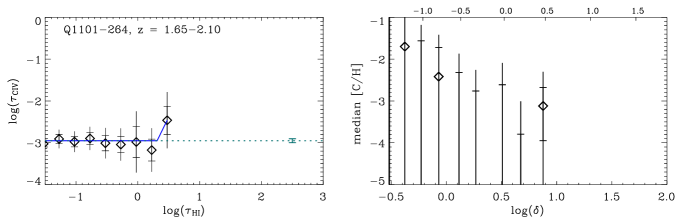
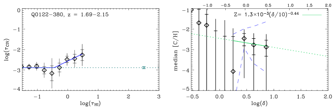
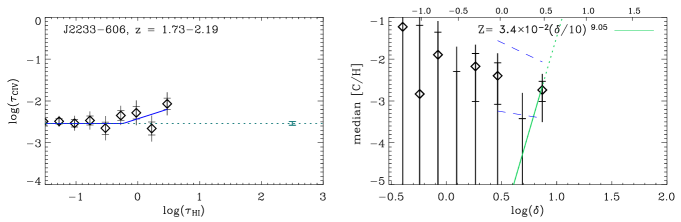
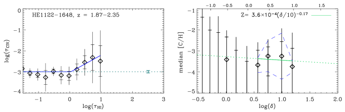
Figure 1.— Results for individual quasars. For each quasar two panels are plotted. Left: Median recovered CIV optical depth as a function of the recovered HI optical depth. The horizontal dotted line indicates $\tau_{\rm min}$; the $1\sigma$ error in this level is indicated on the right-hand side of the panel. The solid line is the best-fit power law, eq. (4). Right: Median carbon abundance $[{\rm C}/{\rm H}]$ as a function of log overdensity. All metallicities were computed as described in §5.1 using the QG UV background. The best-fit power law to the $\tau_{\rm HI}>\tau_{c}$ data points is shown as the solid line (dotted where extrapolated). The dashed lines show the $\pm 1\sigma$ lognormal scatter as measured from the full distribution of pixel optical depths (see §5.2). All data points are shown with both 1 and $2\,\sigma$ error bars.

Continued.

Continued.

Continued.

Continued.

Table 1Recovered CIV optical depths

QSO	$\log\tau_{{\rm HI}}$	$\log\tau_{{\rm CIV}},-0.5\sigma$		$\log\tau_{\rm CIV},{\rm median}$		$\log\tau_{\rm CIV},+0.5\sigma$		$\log\tau_{\rm CIV},+1\sigma$		$\log\tau_{\rm CIV},+1.5\sigma$		$\log\tau_{\rm CIV},+2\sigma$
Q1101-264	-9.000	$\cdots$	$\cdots$	-2.950	0.048	-2.298	0.021	-1. 67	0.022	-1.767	0.015	-1.619	0.028
Q1101-264	-2.775	$\cdots$	$\cdots$	-2.816	-0.481	-2.424	-0.094	-2.092	-0.074	-1.833	-0.058	$\cdots$	$\cdots$
Q1101-264	-2.525	$\cdots$	$\cdots$	-2.856	-0.211	-2.240	-0.062	-1.979	-0.049	-1.787	-0.036	-1.656	-0.070
Q1101-264	-2.275	$\cdots$	$\cdots$	-2.820	-0.119	-2.232	-0.076	-1.929	-0.031	-1.796	-0.029	-1.665	-0.069
Q1101-264	-2.025	$\cdots$	$\cdots$	-2.959	-0.092	-2.334	-0.045	-1.999	-0.029	-1.753	-0.031	-1.615	-0.130
Q1101-264	-1.775	$\cdots$	$\cdots$	-2.887	-0.083	-2.271	-0.035	-1.933	-0.032	-1.758	-0.019	-1.620	-0.027
Q1101-264	-1.525	$\cdots$	$\cdots$	-3.025	-0.117	-2.305	-0.042	-1.961	-0.030	-1.768	-0.029	-1.593	0.029
Q1101-264	-1.275	$\cdots$	$\cdots$	-2.908	-0.111	-2.301	-0.053	-1.966	-0.047	-1.739	-0.030	-1.561	0.078

Note. — Cols. (1) and (2) contain the quasar name and the recovered HI optical depth, respectively. Cols. (3) and (4) contain the 31st percentile of the recovered CIV optical depth and the $1\sigma$ error on this value. Cols. (5)–(14) show the same quantities for higher percentiles (50th, 69th, 84th, 93th, and 98th). An HI optical depth of $\log\tau_{\rm HI}=-9$ indicates that the corresponding $\tau_{\rm CIV}$ are the $\tau_{\rm min}$ values. Negative errors indicate that $\tau_{\rm HI}<\tau_{c}$ (see §5.1 for the definitions of $\tau_{\rm min}$ and $\tau_{c}$). Table 4 is published in its entirety in the electronic edition of the Astrophysical Journal. A portion is shown here for guidance regarding its form and content.

Appendix B B. The observed effective optical depth

Table 1Observed effective optical depth

	All pixels				After removal of contamination
QSO	med$(z)$	$z_{\rm min}$	$z_{\rm max}$	$\tau_{\rm eff}\pm 1\sigma$	med$(z)$	$z_{\rm min}$	$z_{\rm max}$	$\tau_{\rm eff}\pm 1\sigma$
Q1101-264	1.766	1.654	1.878	$0.167\pm 0.025$	1.756	1.654	1.901	$0.099\pm 0.016$
Q1101-264	1.991	1.878	2.103	$0.120\pm 0.022$	2.000	1.901	2.102	$0.093\pm 0.016$
Q0122-380	1.806	1.692	1.919	$0.134\pm 0.021$	1.799	1.692	1.917	$0.120\pm 0.026$
Q0122-380	2.033	1.920	2.147	$0.179\pm 0.024$	2.034	1.917	2.147	$0.162\pm 0.026$
J2233-606	1.848	1.732	1.963	$0.236\pm 0.036$	1.843	1.732	1.964	$0.224\pm 0.033$
J2233-606	2.079	1.963	2.195	$0.128\pm 0.017$	2.080	1.964	2.194	$0.124\pm 0.019$
HE1122-1648	1.990	1.869	2.112	$0.134\pm 0.019$	1.986	1.869	2.108	$0.128\pm 0.019$
HE1122-1648	2.233	2.112	2.355	$0.171\pm 0.025$	2.224	2.108	2.355	$0.164\pm 0.026$
Q0109-3518	1.996	1.874	2.117	$0.199\pm 0.025$	2.003	1.874	2.120	$0.180\pm 0.027$
Q0109-3518	2.239	2.117	2.361	$0.124\pm 0.016$	2.239	2.120	2.361	$0.113\pm 0.018$
HE2217-2818	1.996	1.874	2.117	$0.168\pm 0.024$	1.998	1.874	2.118	$0.139\pm 0.021$
HE2217-2818	2.239	2.117	2.361	$0.160\pm 0.019$	2.242	2.118	2.361	$0.149\pm 0.018$
Q0329-385	2.010	1.888	2.133	$0.117\pm 0.015$	2.010	1.888	2.133	$0.115\pm 0.014$
Q0329-385	2.255	2.133	2.377	$0.156\pm 0.022$	2.256	2.133	2.377	$0.156\pm 0.021$
HE1347-2457	2.108	1.982	2.234	$0.141\pm 0.016$	2.103	1.982	2.243	$0.131\pm 0.019$
HE1347-2457	2.361	2.234	2.487	$0.192\pm 0.024$	2.366	2.243	2.487	$0.175\pm 0.022$
Q1442+293	2.228	2.097	2.359	$0.134\pm 0.017$	2.217	2.097	2.338	$0.137\pm 0.020$
Q1442+293	2.490	2.359	2.621	$0.315\pm 0.041$	2.496	2.338	2.621	$0.214\pm 0.029$
PKS0329-255	2.241	2.109	2.372	$0.186\pm 0.027$	2.243	2.109	2.372	$0.180\pm 0.025$
PKS0329-255	2.504	2.373	2.636	$0.206\pm 0.025$	2.506	2.372	2.636	$0.205\pm 0.022$
Q0002-422	2.307	2.173	2.441	$0.275\pm 0.033$	2.308	2.173	2.434	$0.234\pm 0.029$
Q0002-422	2.576	2.441	2.710	$0.337\pm 0.038$	2.572	2.434	2.710	$0.283\pm 0.032$
HE2347-4342	2.430	2.291	2.569	$0.226\pm 0.029$	2.447	2.291	2.580	$0.177\pm 0.025$
HE2347-4342	2.709	2.569	2.848	$0.305\pm 0.039$	2.715	2.580	2.848	$0.308\pm 0.041$
Q1107+485	2.518	2.375	2.661	$0.195\pm 0.023$	2.509	2.375	2.651	$0.182\pm 0.021$
Q1107+485	2.804	2.661	2.947	$0.314\pm 0.033$	2.805	2.651	2.947	$0.273\pm 0.030$
Q0420-388	2.626	2.479	2.773	$0.294\pm 0.029$	2.626	2.479	2.778	$0.279\pm 0.033$
Q0420-388	2.921	2.773	3.068	$0.360\pm 0.034$	2.920	2.779	3.068	$0.343\pm 0.037$
Q1425+604	2.694	2.544	2.844	$0.417\pm 0.044$	2.670	2.544	2.882	$0.232\pm 0.023$
Q1425+604	2.994	2.844	3.144	$0.363\pm 0.034$	3.009	2.882	3.144	$0.360\pm 0.040$
Q2126-158	2.754	2.601	2.906	$0.437\pm 0.042$	2.752	2.601	2.943	$0.329\pm 0.043$
Q2126-158	3.059	2.906	3.211	$0.310\pm 0.030$	3.078	2.944	3.211	$0.271\pm 0.030$
Q1422+230	3.062	2.898	3.225	$0.417\pm 0.037$	3.058	2.898	3.218	$0.423\pm 0.034$
Q1422+230	3.389	3.225	3.552	$0.512\pm 0.045$	3.382	3.218	3.552	$0.496\pm 0.048$
Q0055-269	3.092	2.928	3.257	$0.381\pm 0.037$	3.088	2.928	3.249	$0.366\pm 0.039$
Q0055-269	3.421	3.257	3.586	$0.426\pm 0.033$	3.411	3.249	3.586	$0.445\pm 0.041$
Q0000-262	3.489	3.312	3.667	$1.107\pm 0.086$	3.708	3.607	3.808	$0.705\pm 0.074$
Q0000-262	3.845	3.667	4.023	$0.758\pm 0.049$	3.912	3.808	4.023	$0.811\pm 0.065$
Q1055+461	3.498	3.320	3.676	$0.595\pm 0.041$	3.517	3.338	3.695	$0.644\pm 0.056$
Q1055+461	3.854	3.676	4.033	$0.774\pm 0.050$	3.862	3.695	4.033	$0.843\pm 0.075$
Q2237-061	3.880	3.690	4.070	$0.828\pm 0.059$	3.862	3.696	4.032	$0.839\pm 0.069$
Q2237-061	4.261	4.070	4.451	$0.890\pm 0.063$	4.287	4.032	4.448	$0.827\pm 0.060$

References

- Aguirre, Schaye, & Theuns (2002) Aguirre, A., Schaye, J., & Theuns, T. 2002, ApJ, 576, 1 (Paper I)
- Aguirre et al. (2001) Aguirre, A., Hernquist, L., Schaye, J., Weinberg, D. H., Katz, N., & Gardner, J. 2001, ApJ, 560, 599
- Aguirre et al. (2001) Aguirre, A., Hernquist, L., Schaye, J., Katz, N., Weinberg, D. H., & Gardner, J. 2001, ApJ, 561, 52
- Anders & Grevesse (1989) Anders, E. & Grevesse, N. 1989, Geochim. Cosmochim. Acta, 53, 197
- Barlow & Sargent (1997) Barlow, T. A. & Sargent, W. L. W. 1997, AJ, 113, 136
- Bergeron, Aracil, Petitjean, & Pichon (2002) Bergeron, J., Aracil, B., Petitjean, P., & Pichon, C. 2002, A&A, 396, L11
- Bernardi et al. (2003) Bernardi, M. et al. 2003, AJ, 125, 32
- Bi & Davidsen (1997) Bi, H. & Davidsen, A. F. 1997, ApJ, 479, 523
- Boksenberg, Sargent, & Rauch (2003) Boksenberg, A., Sargent, W. L. W., & Rauch, M. 2003, ApJS, submitted (astro-ph/0307557)
- Bromm, Ferrara, Coppi, & Larson (2001) Bromm, V., Ferrara, A., Coppi, P. S., & Larson, R. B. 2001, MNRAS, 328, 969
- Carswell et al. (1984) Carswell, R. F., Morton, D. C., Smith, M. G., Stockton, A. N., Turnshek, D. A., & Weymann, R. J. 1984, ApJ, 278, 486
- Carswell, Schaye, & Kim (2002) Carswell, B., Schaye, J., & Kim, T. 2002, ApJ, 578, 43
- Cen & Ostriker (1999) Cen, R. & Ostriker, J. P. 1999, ApJ, 519, L109
- Cowie & Songaila (1998) Cowie, L. L. & Songaila, A. 1998, Nature, 394, 44
- Cowie, Songaila, Kim, & Hu (1995) Cowie, L. L., Songaila, A., Kim, T., & Hu, E. M. 1995, AJ, 109, 1522
- Croft, Weinberg, Katz, & Hernquist (1997) Croft, R. A. C., Weinberg, D. H., Katz, N., & Hernquist, L. 1997, ApJ, 488, 532
- Davé et al. (1998) Davé, R., Hellsten, U., Hernquist, L., Katz, N., & Weinberg, D. H. 1998, ApJ, 509, 661
- D’Odorico et al. (2000) D’Odorico, S., Cristiani, S., Dekker, H., Hill, V., Kaufer, A., Kim, T., & Primas, F. 2000, Proc. SPIE, 4005, 121
- Ellison et al. (1999) Ellison, S. L., Lewis, G. F., Pettini, M., Chaffee, F. H., & Irwin, M. J. 1999, ApJ, 520, 456
- Ellison, Songaila, Schaye, & Pettini (2000) Ellison, S. L., Songaila, A., Schaye, J., & Pettini, M. 2000, AJ, 120, 1175
- Ferland (2000) Ferland, G. J. 2000, Revista Mexicana de Astronomia y Astrofisica Conference Series, 9, 153
- Ferland et al. (1998) Ferland, G. J., Korista, K. T., Verner, D. A., Ferguson, J. W., Kingdon, J. B., & Verner, E. M. 1998, PASP, 110, 761
- Furlanetto & Loeb (2003) Furlanetto, S. R. & Loeb, A. 2003, ApJ, 588, 18
- Haardt & Madau (1996) Haardt, F. & Madau, P. 1996, ApJ, 461, 20
- Haardt & Madau (2001) Haardt, F., & Madau, P. 2001, to be published in the proceedings of XXXVI Rencontres de Moriond, astro-ph/0106018
- Haehnelt, Steinmetz, & Rauch (1996) Haehnelt, M. G., Steinmetz, M., & Rauch, M. 1996, ApJ, 465, L95
- Heap et al. (2000) Heap, S. R., Williger, G. M., Smette, A., Hubeny, I., Sahu, M. S., Jenkins, E. B., Tripp, T. M., & Winkler, J. N. 2000, ApJ, 534, 69
- Hellsten et al. (1997) Hellsten, U., Dave, R., Hernquist, L., Weinberg, D. H., & Katz, N. 1997, ApJ, 487, 482
- Kim, Cristiani, & D’Odorico (2001) Kim, T.-S., Cristiani, S., & D’Odorico, S. 2001, A&A, 373, 757
- Kim et al. (2002) Kim, T.-S., Carswell, R. F., Cristiani, S., D’Odorico, S., & Giallongo, E. 2002, MNRAS, 335, 555
- Kim et al. (2002) Kim, T.-S., Viel, M., & Haehnelt, M., Carswell, R. F., & Cristiani, S. 2003, MNRAS, (astro-ph/0308103)
- Kriss et al. (2001) Kriss, G. A. et al. 2001, Science, 293, 1112
- Madau, Ferrara, & Rees (2001) Madau, P., Ferrara, A., & Rees, M. J. 2001, ApJ, 555, 92
- Pettini et al. (2003) Pettini, M., Madau, P., Bolte, M., Prochaska, J. X., Ellison, S. L., & Fan, X. 2003, ApJ, in press (astro-ph/0305413)
- Rauch, Sargent, Womble, & Barlow (1996) Rauch, M., Sargent, W. L. W., Womble, D. S., & Barlow, T. A. 1996, ApJ, 467, L5
- Rauch, Haehnelt, & Steinmetz (1997) Rauch, M., Haehnelt, M. G., & Steinmetz, M. 1997, ApJ, 481, 601
- Rauch et al. (1997) Rauch, M. et al. 1997, ApJ, 489, 7
- Rollinde, Petitjean, & Pichon (2001) Rollinde, E., Petitjean, P., & Pichon, C. 2001, A&A, 376, 28
- Scannapieco, Ferrara, & Madau (2002) Scannapieco, E., Ferrara, A., & Madau, P. 2002, ApJ, 574, 590
- Scannapieco, Schneider, & Ferrara (2003) Scannapieco, E., Schneider, R., & Ferrara, A. 2003, ApJ, 589, 35
- Schaye (2001) Schaye, J. 2001, ApJ, 559, 507
- Schaye, Theuns, Leonard, & Efstathiou (1999) Schaye, J., Theuns, T., Leonard, A., & Efstathiou, G. 1999, MNRAS, 310, 57
- Schaye, Rauch, Sargent, & Kim (2000) Schaye, J., Rauch, M., Sargent, W. L. W., & Kim, T. 2000a, ApJ, 541, L1
- Schaye et al. (2000) Schaye, J., Theuns, T., Rauch, M., Efstathiou, G., & Sargent, W. L. W. 2000b, MNRAS, 318, 817
- Schneider, Ferrara, Natarajan, & Omukai (2002) Schneider, R., Ferrara, A., Natarajan, P., & Omukai, K. 2002, ApJ, 571, 30
- Simcoe, Sargent, & Rauch (2002) Simcoe, R. A., Sargent, W. L. W., & Rauch, M. 2002, ApJ, 578, 737
- Songaila (1998) Songaila, A. 1998, AJ, 115, 2184
- Songaila (2001) Songaila, A. 2001, ApJ, 561, L153
- Songaila & Cowie (1996) Songaila, A. & Cowie, L. L. 1996, AJ, 112, 335
- Spergel et al. (2003) Spergel, D. N., et al. 2003, ApJ, in press (astro-ph/0302209)
- Telfer et al. (2002) Telfer, R. C., Kriss, G. A., Zheng, W., Davidsen, A. F., & Tytler, D. 2002, ApJ, 579, 500
- Thacker, Scannapieco, & Davis (2002) Thacker, R. J., Scannapieco, E., & Davis, M. 2002, ApJ, 581, 836
- Theuns, Schaye, & Haehnelt (2000) Theuns, T., Schaye, J., & Haehnelt, M. G. 2000, MNRAS, 315, 600
- Theuns et al. (2002a) Theuns, T., Schaye, J., Zaroubi, S., Kim, T., Tzanavaris, P., & Carswell, B. 2002a, ApJ, 567, L103
- Theuns et al. (2002b) Theuns, T., Viel, M., Kay, S., Schaye, J., Carswell, R. F., & Tzanavaris, P. 2002b, ApJ, 578, L5
- Vogt et al. (1994) Vogt, S. S. et al. 1994, Proc. SPIE, 2198, 362
- Zhang, Meiksin, Anninos, & Norman (1998) Zhang, Y., Meiksin, A., Anninos, P., & Norman, M. L. 1998, ApJ, 495, 63