Gravitational lensing as a probe of structure

Abstract

Gravitational lensing has become one of the most interesting tools to study the mass distribution in the Universe. Since gravitational light deflection is independent of the nature and state of the matter, it is ideally suited to investigate the distribution of all (and thus also of dark) matter in the Universe. Lensing results have now become available over a wide range of scales, from the search for MACHOs in the Galactic halo, to the mass distribution in galaxies and clusters of galaxies, and the statistical properties of the large-scale matter distribution in the Universe. Here, after introducing the concepts of strong and weak lensing, several applications are outlined, from strong lensing by galaxies, to strong and weak lensing by clusters and the lensing properties of the large-scale structure.

1 Introduction

Light rays are deflected in gravitational fields, just like massive particles are. Hence, the deflection of light probes the gravitational field, and therefore the matter distribution that causes it. Since the field is independent of the state and nature of the matter generating it, it provides an ideal tool for studying the total (that is, luminous and dark) matter in cosmic objects. As we shall see, gravitational light deflection is used to study cosmic mass distributions on scales ranging from stars to galaxies, and from clusters of galaxies to the large-scale matter distribution in the Universe. In this contribution, I will concentrate on those aspects which are of particular relevance for learning about the dark matter distribution in the Universe.

Gravitational lensing describes phenomena of gravitational light deflection in the weak-field, small deflection limit; strong-field light deflection (important for light propagation near black holes or neutron stars) are not covered by gravitational lens (hereafter GL) theory. The basic theory of gravity, and of light propagation in a gravitational field is General Relativity, which says that photons travel along null geodesics of the spacetime metric (these are described by a second-order differential equation). In GL theory, several simplifications apply, owing to restriction to weak fields, and thus small deflections. We shall see the convenience of those further below.

Gravitational lensing as a whole, and several particular aspects of it, has been reviewed previously. Two extensive monographs (Schneider, Ehlers & Falco 1992, hereafter SEF; Petters, Levine & Wambsganss 2001, hereafter PLW) describe lensing in all depth, in particular providing a derivation of the gravitational lensing equations from General Relativity. Fort & Mellier (1994) describe the giant luminous arcs and arclets in clusters of galaxies (see Sect. 5.3), Paczyński (1996) and Roulet & Mollerach (1997) review the effects of gravitational microlensing in the Local Group, whereas the reviews by Narayan & Bartelmann (1999) and Wambsganss (1998) provide a concise and didactical account of GL theory and observations. Much of this contribution will be focused on weak gravitational lensing, which has been reviewed recently by Mellier (1999), Bartelmann & Schneider (2001), Wittman (2002), van Waerbeke & Mellier (2003) and Refregier (2003).

2 Basics of gravitational lensing

2.1 Very brief history of lensing

The investigation of gravitational light deflection dates back more than 200 years to Mitchel, Cavendish, Laplace and Soldner (see SEF, PLW for references and much more detail). At that time a metric theory of gravity was not known, and light was treated as massive particles moving with the velocity of light. General Relativity, finalized in 1915, predicts a deflection angle twice as large as ‘Newtonian’ theory, and was verified in 1919 by measuring the deflection of light near the Solar limb during an eclipse. Soon after, the ‘lens effect’ was discussed by Lodge, Eddington and Chwolson, i.e. the possibility that light deflection leads to multiple images of sources behind mass concentrations, or even yields a ring-like image. Einstein, in 1936, considered in detail the lensing of a source by a star (or a point-mass lens), and concluded that the angular separation between the two images would be far too small (of order milliarcseconds) to be resolvable, so that “there is no great chance of observing this phenomenon”. In 1937, Zwicky, instead of looking at lensing by stars in our Galaxy, considered “extragalactic nebulae” (nowadays called galaxies) as lenses. He noted that they produce angular separations than can be separated with telescopes. Observing such an effect, he noted, would furnish an additional test of GR, would allow one to see galaxies at larger distances (due to the magnification effect), and to determine the masses of these nebulae acting as lenses. He furthermore considered the probability of such lens effects and concluded that about 1 out of 400 distant sources should be affected by lensing, and therefore predicted that “the probability that nebulae which act as gravitational lenses will be found becomes practically a certainty”. His visions were right on (nearly) all accounts.

In the mid-1960’s, Klimov, Liebes, and Refsdal independently formulated the basic theory of gravitational lensing, and focused on astrophysical applications, like determination of masses and cosmological parameters. For example, Refsdal noticed that the light travel time along the two rays corresponding to two images of a source, is proportional to the size of the Universe, thus to $H_{0}^{-1}$, and that a measurement of the time delay, possible if the source varies intrinsically, would allow the determination of the Hubble constant.

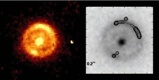
Figure 1: The radio source JVAS B1938+666 shows two radio sources (contours in the right panel), one of which is mapped into four components, the other shows a double image; furthermore, the outer radio contours merge into an arc around the lensing galaxy. The underlying grey-scale figure, and the left panel, shows a near-IR iamge of the field, revealing the lens galaxy, as well as the Einstein-ring image of the galaxy hosting the radio-AGN (from King et al. 1998)

In 1979, the first GL system was discovered by Walsh, Carswell & Weymann: The two images of the QSO 0957+561 are separated by about 6 arcseconds, having identical colors, redshifts ($z_{\rm s}=1.41$) and spectra; both images are radio sources with a core-jet structure on milli-arcsec scales. Soon thereafter, a galaxy situated between the two quasar images was detected, with redshift $z_{\rm d}=0.36$, being member of a cluster. 1980 marks the discovery of the first GL system with four QSO images, QSO 1115+080, two of which are very closely spaced. 1986 saw the discovery of a new lensing phenomenon, which had been predicted long before: the detection of a radio ring, in which an extended radio source is mapped into a complete ring by an intervening galaxy (see also Fig. 1). Such Einstein rings turn out to yield the most accuracte mass determinations in extragalactic astronomy. At present, some 72 multiple-image systems are known where the major lens component is a galaxy, including about 46 doubles, 20 four-image systems, but also one 3-image, one 5-image, and one 6-image system. The first of these were discovered serendipitously, but since the 1990’s, large systematic searches for such systems were successfully conducted in the optical and, in particular, radio wavebands.

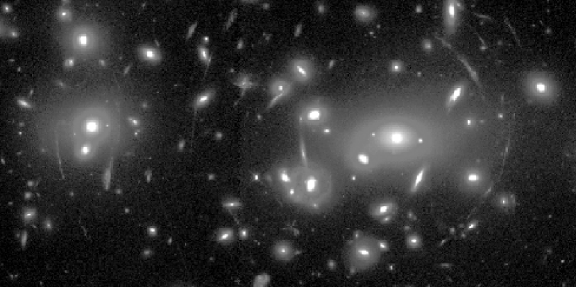
Figure 2: The redshift $z=0.18$ cluster Abell 2218 displays an enormously rich structure of arcs, highly stretched images of background galaxies which curve around the main cluster center (seen to the right of the image center), but also around the secondary mass peak near the left edge of this WFPC2@HST image. Together with the identification of several multiply-imaged background sources, these lensing phenomena have yielded a very detailed mass map of the inner part of this cluster (Courtesy J.-P. Kneib)

In 1986, a new lensing phenomenon was discovered by two independent groups: strongly elongated, curved features around two clusters of galaxies. Their extreme length-to-width ratios made them difficult to interpret; the measurement of the redshift of one of them placed the source of the arc at a distance well behind the corresponding cluster. Hence, these giant luminous arcs are images of background galaxies, highly distorted by the tidal gravitational field of the cluster. By now, many clusters with giant arcs are known and investigated in detail, for which in particular the high-resolution of the HST was essential. Less extremely distorted images of background galaxies have been named arclets and can be identified in many clusters.

If some sources are so highly distorted as those seen in Fig. 2, one expects to see many more sources which are distorted to a much smaller degree – such that they can not be identified individually as lensed images, but that nearby images are distorted in a similar way, so that the distortion can be identified statistically. This forms the basis of weak lensing; coherent image distortions around massive clusters were detected in the early 1990’s by Tyson and his group. As shown by Kaiser & Squires, there image distortions can be used to obtain a parameter-free mass map of clusters. Further weak lensing phenomena, such as galaxy-galaxy lensing, have been detected in the last decade; the weak lensing effect by the large-scale matter distribution in the Universe, the so-called cosmic shear, was discovered by several independent teams simultaneously in 2000, and this has opened up a new window in observational cosmology.

Last but not least, gravitational microlensing in the local group has been suggested in 1986 by Paczynski as a test of whether the dark matter in the halo of our Galaxy is made up of compact objects; the first microlensing events were discovered in 1993 by three different groups. I refer to the lectures of Prof. Sadoulet for a discussion of microlensing and the results concerning the dark matter in our Milky Way.

2.2 Deflection angle and lens equation

We shall provide here the basic lensing relations; the reader is encouraged to refer to one of the reviews or books listed in the introduction for a full derivation of these relations.

2.2.1 Deflection by a ‘point mass’ $M$

Consider the deflection of a light ray by the exterior of a spherically symmetric mass $M$; from the Schwarzschild metric one finds that a ray with impact parameter $\xi$ is deflected by an angle

$$\framebox{$\displaystyle\hat{\alpha}=\frac{4GM}{c^{2}\,\xi}={2R_{\rm s}\over\xi}$}\;:\;\;\hbox{Einstein deflection angle;}\;\;\hbox{$R_{\rm s}$: Schwarzschild radius}$$ (2.1)

valid for $R_{\rm s}/\xi\ll 1$, or $\hat{\alpha}\ll 1$; note that this also implies that $\Phi/c^{2}\ll 1$, where $\Phi$ is the Newtonian gravitational potential. The value for $\hat{\alpha}$ is twice the ‘Newtonian’ value derived by Soldner and others and was verified during the Solar Eclipse 1919!

2.2.2 Deflection by a mass distribution

Since the field equations of General Relativity can be linearized if the gravitational field is weak, the deflection angle caused by an extended mass distribution can be calculated as the (vectorial) sum of the deflections due to its individual mass elements. If the deflection angle is small (which is implied by the weak-field assumption), the light ray near the mass distribution will deviate only slightly from the straight, undeflected ray. In this (‘Born’) approximation, valid if the extent of the mass distribution is much smaller than the distances between source, lens, and observer (the ‘geometrically thin lens’), the deflection angle depends solely on the surface mass density $\Sigma({\hbox{$\bf\xi$}})$, defined in terms of the volume density $\rho(\vec{r})$ as

$$\Sigma({\hbox{$\bf\xi$}})\equiv\int{\rm d}r_{3}\,\rho(\xi_{1},\xi_{2},r_{3})\;,$$ (2.2)

with the $r_{3}$-direction along the line-of-sight. Superposing the deflections by the mass elements of the lens, one obtains the deflection angle

$$\framebox{$\displaystyle\hat{{\hbox{$\bf\alpha$}}}({\hbox{$\bf\xi$}})=\frac{4G}{c^{2}}\,\int{\rm d}^{2}\xi^{\prime}\,\Sigma({\hbox{$\bf\xi$}}^{\prime})\,\frac{{\hbox{$\bf\xi$}}-{\hbox{$\bf\xi$}}^{\prime}}{|{\hbox{$\bf\xi$}}-{\hbox{$\bf\xi$}}^{\prime}|^{2}}$}\;.$$ (2.3)

The geometrically-thin condition is satisfied in virtually all astrophysically relevant situations (i.e. lensing by galaxies and clusters of galaxies), unless the deflecting mass extends all the way from the source to the observer, as in the case of lensing by the large-scale structure. The relevant deflections are small, e.g., $\hat{\alpha}\mathrel{\mathchoice{\lower 2.0pt\vbox{\halign{$\m@th\displaystyle\hfil#\hfil$\cr<\crcr\sim\crcr}}}{\lower 2.0pt\vbox{\halign{$\m@th\textstyle\hfil#\hfil$\cr<\crcr\sim\crcr}}}{\lower 2.0pt\vbox{\halign{$\m@th\scriptstyle\hfil#\hfil$\cr<\crcr\sim\crcr}}}{\lower 2.0pt\vbox{\halign{$\m@th\scriptscriptstyle\hfil#\hfil$\cr<\crcr\sim\crcr}}}}1^{\prime\prime}$ for galaxies, $\hat{\alpha}\mathrel{\mathchoice{\lower 2.0pt\vbox{\halign{$\m@th\displaystyle\hfil#\hfil$\cr<\crcr\sim\crcr}}}{\lower 2.0pt\vbox{\halign{$\m@th\textstyle\hfil#\hfil$\cr<\crcr\sim\crcr}}}{\lower 2.0pt\vbox{\halign{$\m@th\scriptstyle\hfil#\hfil$\cr<\crcr\sim\crcr}}}{\lower 2.0pt\vbox{\halign{$\m@th\scriptscriptstyle\hfil#\hfil$\cr<\crcr\sim\crcr}}}}30^{\prime\prime}$ for clusters.

2.2.3 The lens equation

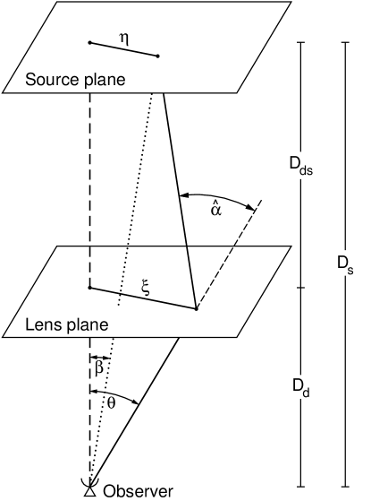
Figure 3: Sketch of a typical gravitational lens system.

The lens equation relates the true position of the source to its observed position; we define the lens and source plane as planes perpendicular to the line-of-sight to the deflector, at the distance $D_{\rm d}$ and $D_{\rm s}$ of the lens and the source, respectively (see Fig. 3). Furthermore, we define the ‘optical axis’ as a ‘straight’ line through the lens center (the exact definition does not matter; any change of it represents just an unobservable translation in the source plane), and its intersections with the lens and source planes as their respective origins. Denoting $\bf\xi$ as the two-dimensional position of the light ray in the lens plane and $\bf\eta$ as the position of the source (see Fig. 3), then from geometry,

$${\hbox{$\bf\eta$}}={D_{\rm s}\over D_{\rm d}}\,{\hbox{$\bf\xi$}}-D_{\rm ds}\hat{{\hbox{$\bf\alpha$}}}({\hbox{$\bf\xi$}})\;.$$ (2.4)

Note that the distances $D$ occuring here are the angular-diameter distances, since they relate physical transverse separations to angles. If $\bf\theta$ denotes the angle of a light ray relative to the optical axis, $\bf\beta$ as the angular position of the unlensed source (see Fig. 3),

$${\hbox{$\bf\eta$}}=D_{\rm s}{\hbox{$\bf\beta$}}\;;\;{\hbox{$\bf\xi$}}=D_{\rm d}{\hbox{$\bf\theta$}}\;,$$ (2.5)

then

$$\framebox{$\displaystyle{\hbox{$\bf\beta$}}={\hbox{$\bf\theta$}}-\frac{D_{\rm ds}}{D_{\rm s}}\,\hat{{\hbox{$\bf\alpha$}}}(D_{\rm d}{\hbox{$\bf\theta$}})\equiv{\hbox{$\bf\theta$}}-{\hbox{$\bf\alpha$}}({\hbox{$\bf\theta$}})$}\;,$$ (2.6)

where ${\hbox{$\bf\alpha$}}({\hbox{$\bf\theta$}})$ is the scaled deflection angle, which in terms of the dimensionless surface mass density

$$\framebox{$\displaystyle\kappa({\hbox{$\bf\theta$}}):=\frac{\Sigma(D_{\rm d}{\hbox{$\bf\theta$}})}{\Sigma_{\rm cr}}$}\quad\hbox{with}\quad\framebox{$\displaystyle\Sigma_{\rm cr}=\frac{c^{2}}{4\pi G}\,\frac{D_{\rm s}}{D_{\rm d}\,D_{\rm ds}}$}\;,$$ (2.7)

reads as

$$\framebox{$\displaystyle{\hbox{$\bf\alpha$}}({\hbox{$\bf\theta$}})=\frac{1}{\pi}\,\int_{{\rm I\mathchoice{\kern-1.99168pt}{\kern-1.99168pt}{\kern-1.84941pt}{\kern-1.42262pt}R}^{2}}{\rm d}^{2}\theta^{\prime}\,\kappa({\hbox{$\bf\theta$}}^{\prime})\,\frac{{\hbox{$\bf\theta$}}-{\hbox{$\bf\theta$}}^{\prime}}{|{\hbox{$\bf\theta$}}-{\hbox{$\bf\theta$}}^{\prime}|^{2}}$}\;.$$ (2.8)

Note that the critical surface mass density $\Sigma_{\rm cr}$ depends only on the distances. Lenses with $\kappa\sim 1$ at some points are called strong lenses, and those with $\kappa\ll 1$ everywhere are weak lenses. The lens equation ${\hbox{$\bf\beta$}}={\hbox{$\bf\theta$}}-{\hbox{$\bf\alpha$}}({\hbox{$\bf\theta$}})$ is a mapping ${\hbox{$\bf\theta$}}\to{\hbox{$\bf\beta$}}$ from the lens plane to the source plane; but in general, this mapping is non-invertable: for a given source position $\bf\beta$, the lens equation can have multiple solutions $\bf\theta$ which correspond to multiple images of a source at $\bf\beta$.

2.2.4 Deflection and Fermat potentials

Since $\nabla\ln|{\hbox{$\bf\theta$}}|={\hbox{$\bf\theta$}}/|{\hbox{$\bf\theta$}}|^{2}$, the deflection angle can be written as

$$\framebox{$\displaystyle{\hbox{$\bf\alpha$}}=\nabla\psi$}\;,\quad{\rm with}\quad\framebox{$\displaystyle\psi({\hbox{$\bf\theta$}})={1\over\pi}\int_{{\rm I\mathchoice{\kern-1.99168pt}{\kern-1.99168pt}{\kern-1.84941pt}{\kern-1.42262pt}R}^{2}}{\rm d}^{2}\theta^{\prime}\;\kappa({\hbox{$\bf\theta$}}^{\prime})\,\ln|{\hbox{$\bf\theta$}}-{\hbox{$\bf\theta$}}^{\prime}|$}\;;$$ (2.9)

being the deflection potential; hence, the lens equation describes a gradient mapping. From $\nabla^{2}\ln|{\hbox{$\bf\theta$}}|=2\pi\delta_{\rm D}({\hbox{$\bf\theta$}})$, where $\delta_{\rm D}$ denotes Dirac’s delta-‘function’, one finds the 2-D Poisson equation

$$\framebox{$\displaystyle\nabla^{2}\psi=2\kappa$}\;.$$ (2.10)

Defining the Fermat potential

$$\phi({\hbox{$\bf\theta$}};{\hbox{$\bf\beta$}})={1\over 2}\left({\hbox{$\bf\theta$}}-{\hbox{$\bf\beta$}}\right)^{2}-\psi({\hbox{$\bf\theta$}})\;,$$ (2.11)

where $\bf\beta$ enters as a parameter, one sees that the lens equation can be written as

$$\nabla\phi({\hbox{$\bf\theta$}};{\hbox{$\bf\beta$}})={\hbox{$\bf 0$}}\;.$$ (2.12)

Solutions of (2.12) can then be classified, according to whether the potential $\phi$ has a minimum, maximum, or saddle point at the solution point $\bf\theta$.

2.3 Effects of lensing

2.3.1 Multiple images

Multiple images correspond to multiple solutions $\bf\theta$ of the lens equation for fixed source position $\bf\beta$. For the case of a point-mass lens,

$$\hat{{\hbox{$\bf\alpha$}}}({\hbox{$\bf\xi$}})={4GM\over c^{2}}\,{{\hbox{$\bf\xi$}}\over|{\hbox{$\bf\xi$}}|^{2}}\;,\quad{\hbox{$\bf\beta$}}={\hbox{$\bf\theta$}}-{4GMD_{\rm ds}\over c^{2}\,D_{\rm d}D_{\rm s}}{{\hbox{$\bf\theta$}}\over|{\hbox{$\bf\theta$}}|^{2}}={\hbox{$\bf\theta$}}-\theta_{\rm E}^{2}{{\hbox{$\bf\theta$}}\over|{\hbox{$\bf\theta$}}|^{2}}\;,$$ (2.13)

where $\theta_{\rm E}$ is the Einstein angle $\propto\sqrt{M}$. Note that (2.13) can also be obtained from (2.3) and (2.6) by setting $\Sigma({\hbox{$\bf\xi$}})=M\,\delta_{\rm D}({\hbox{$\bf\xi$}})$. The lens equation has two solutions, one on either side of the lens (just solve the quadratic equation for $\theta$), with image separation $\Delta\theta\mathrel{\mathchoice{\lower 2.0pt\vbox{\halign{$\m@th\displaystyle\hfil#\hfil$\cr>\crcr\sim\crcr}}}{\lower 2.0pt\vbox{\halign{$\m@th\textstyle\hfil#\hfil$\cr>\crcr\sim\crcr}}}{\lower 2.0pt\vbox{\halign{$\m@th\scriptstyle\hfil#\hfil$\cr>\crcr\sim\crcr}}}{\lower 2.0pt\vbox{\halign{$\m@th\scriptscriptstyle\hfil#\hfil$\cr>\crcr\sim\crcr}}}}2\theta_{\rm E}\propto\sqrt{M}$. Hence, the image separation yields an estimate for the mass of the lens. In general, however, more complicated mass models are needed to fit the observed image positions in a gravitational lens system, i.e., to find a mass model and a source position such that ${\hbox{$\bf\beta$}}={\hbox{$\bf\theta$}}_{i}-{\hbox{$\bf\alpha$}}({\hbox{$\bf\theta$}}_{i})$ is satisfied for all images ${\hbox{$\bf\theta$}}_{i}$.

2.3.2 Magnification

Gravitational light deflection conserves surface brightness; this follows from Liouville’s theorem, noting that light deflection is not associated with emission or absorption processes. Therefore, $I({\hbox{$\bf\theta$}})=I^{(\rm s)}[{\hbox{$\bf\beta$}}({\hbox{$\bf\theta$}})]$, where $I({\hbox{$\bf\theta$}})$ and $I^{(\rm s)}({\hbox{$\bf\beta$}})$ denote the surface brightness in the image and source plane. Differential light bending causes light bundles to get distorted; for very small light bundles, the distortion is described by the Jacobian matrix

$${\mathcal{A}}({\hbox{$\bf\theta$}})=\frac{\partial{\hbox{$\bf\beta$}}}{\partial{\hbox{$\bf\theta$}}}=\left(\delta_{ij}-\frac{\partial^{2}\psi({\hbox{$\bf\theta$}})}{\partial\theta_{i}\partial\theta_{j}}\right)=\left(\begin{array}[]{cc}1-\kappa-\gamma_{1}&-\gamma_{2}\\ -\gamma_{2}&1-\kappa+\gamma_{1}\\ \end{array}\right)\;,$$ (2.14)

where

$$\gamma_{1}=\frac{1}{2}(\psi_{,11}-\psi_{,22})\;,\quad\gamma_{2}=\psi_{,12}\;$$ (2.15)

are the two Cartesian components of the shear (or the tidal gravitational force). For a small source centered on ${\hbox{$\bf\beta$}}_{0}={\hbox{$\bf\theta$}}_{0}-{\hbox{$\bf\alpha$}}({\hbox{$\bf\theta$}}_{0})$:

$$I({\hbox{$\bf\theta$}})=I^{(\rm s)}\left[{\hbox{$\bf\beta$}}_{0}+{\mathcal{A}}({\hbox{$\bf\theta$}}_{0})\cdot({\hbox{$\bf\theta$}}-{\hbox{$\bf\theta$}}_{0})\right]\;.$$ (2.16)

Hence, the image of a small circular source with radius $r$ is an ellipse with semi-axes $\lambda_{1,2}\,r$ where $\lambda_{1,2}$ are the eigenvalues of ${\cal A}$; the orientation of the ellipse is determined by the shear components $\gamma_{1,2}$.

The area distortion by differential deflection yields a magnification (since $I$ is unchanged, and ${\rm flux}=I\times\hbox{solid angle}$),

$$\framebox{$\displaystyle\mu={S\over S_{0}}=\frac{1}{\det{\mathcal{A}}}=\frac{1}{(1-\kappa)^{2}-|\gamma|^{2}}$}\;,$$ (2.17)

with $|\gamma|=\sqrt{\gamma_{1}^{2}+\gamma_{2}^{2}}$. Since ${\cal A}$ is different for different multiple images, the image fluxes are different; the observed flux ratios yield the image magnification ratios. In particular, if the image separation in a point mass lens system is substantially larger than $2\theta_{\rm E}$, which occurs for $|{\hbox{$\bf\beta$}}|\gg\theta_{\rm E}$, the secondary image is very strongly demagnified and thus invisible. Flux ratios can in principle be used to constrain lens models, in addition to the image positions, but the magnifications are affected by small-scale structure in the mass distribution (we shall come back to this point below), rendering them less useful in mass model determinations. Note that the final expression in (2.17) can have either sign; images with $\mu>0$ have positive parity, those with $\mu<0$ negative parity. Positive parity images correspond to extrema of the Fermat potential $\phi$, negative parity images correspond to saddle points of $\phi$. In the rest of this article, we will always mean the absolute value of the magnification when writing $\mu$.

2.3.3 Shape distortions

The image shape of extended (resolved) sources is changed by lensing, since the eigenvalues of ${\cal A}$ are different in general; rewriting

$$\framebox{$\displaystyle{\mathcal{A}}({\hbox{$\bf\theta$}})=(1-\kappa)\left(\begin{array}[]{cc}1-g_{1}&-g_{2}\\ -g_{2}&1+g_{1}\\ \end{array}\right)$}\;,\;\framebox{$\displaystyle g_{i}={\gamma_{i}\over(1-\kappa)}$}:\;\hbox{reduced shear}\;,$$ (2.18)

one sees that the shape distortion is determined by the reduced shear. This in fact forms the basis of weak lensing. It should be noted that giant arcs cannot be described by the linearized lens equation, as they are too big.

2.3.4 Time delay

The light travel time along the various ray paths corresponding to different images is different in general. This implies that variations of the source luminosity will show up as flux variations of the different images at different times, shifted by a time delay $\Delta t$,

$$\Delta t={D_{\rm d}D_{\rm s}\over c\,D_{\rm ds}}(1+z_{\rm d})\left[\phi({\hbox{$\bf\theta$}}^{(1)};{\hbox{$\bf\beta$}})-\phi({\hbox{$\bf\theta$}}^{(2)};{\hbox{$\bf\beta$}})\right]\;,$$ (2.19)

where ${\hbox{$\bf\theta$}}^{(1)}$ and ${\hbox{$\bf\theta$}}^{(2)}$ are the two image positions considered. In fact, $\phi({\hbox{$\bf\theta$}};{\hbox{$\bf\beta$}})$ is, up to an affine transformation, the light travel time along a ray from the source at $\bf\beta$ which crosses the lens plane at $\bf\theta$. Recalling that $\nabla\phi({\hbox{$\bf\theta$}};{\hbox{$\bf\beta$}})=0$ was equivalent to the lens equation, we see from (2.19) that this is Fermat’s principle in lensing: the light travel time is stationary at physical images. Note that $\Delta t\propto H_{0}^{-1}$, since all the distances $D$ are $\propto c/H_{0}$; hence, a measurement of the time delay can be used to determine the Hubble constant, provided the lens model is sufficiently well known. We shall return to this issue below.

2.3.5 General properties of lenses

If $\Sigma({\hbox{$\bf\xi$}})$ is a smooth function, then for (nearly) every source position $\bf\beta$, the number of images is odd (‘odd-number theorem’; Burke 1981). If in addition, $\Sigma({\hbox{$\bf\xi$}})$ is non-negative, then at least one of the images (corresponding to a minimum in light travel time) is magnified, $\mu\geq 1$ (‘magnification theorem’; Schneider 1984). The odd-number theorem is violated observationally: one (usually) finds doubles and quads. The missing odd image is expected to be close to the center of the lens, where $\kappa\gg 1$ presumably, meaning that $\mu\ll 1$; hence, this central image is highly demagnified, and thus not observable. Both of these theorems can be generalized even to non-thin lenses (Seitz & Schneider 1992).

The closed and smooth curves where $\det{\cal A}({\hbox{$\bf\theta$}})=0$ are called critical curves. When they are mapped back into the source plane using the lens equation, the corresponding curves in the source plane are called caustics.

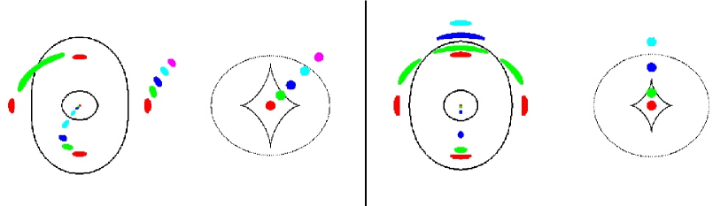
Figure 4: Illustration of critical curves and caustics for an elliptical mass distribution, and the image geometry for various source positions (taken from Narayan & Bartelmann 1999). In each of the two panels, the right figure shows the caustic curves, together with several different source positions; the corresponding image positions are displayed on the left, together with the critical curves. One sees that, depending on where the source is located relative to the caustics, different image multiplicities occur

The number of images changes by $\pm 2$ if the source position crosses a caustic; then two images appear or merge. A source close to, and at the inner side of, a caustic produces two closely separated and very bright images near the corresponding critical curve. A source close to, and on the inner side of a cusp has three bright images close to the corresponding point on the critical curve. From singularity theory, one finds that in the limit of very large magnifications, the two close images on either side of the critical curve have equal magnification, and thus should appear equally bright. Similarly, of the three images formed near a cusp, the sum of the magnifications of the outer two images should equal that of the middle image, with corresponding consequences for the flux ratios. As we shall see, these universality relations are strongly violated in observed lens systems, providing a strong clue for the presence of substructure in the mass distribution of lens galaxies.

3 (Strong) Lensing by galaxies

The first lensing phenomena detected were multiple images of distant QSOs caused by the lensing effect of a foreground galaxy. If the lens is a massive (i.e., $\sim L_{*}$) galaxy, the corresponding image separations are $\sim 1^{\prime\prime}$. Gravitational lens models can be used to constrain the mass distribution in (the inner part of) these lensing galaxies; in particular, the mass inside a circle traced by the multiple images (or the Einstein ring) can be determined with very high precision in some cases. Furthermore, as already mentioned, time-delays can be used to determine $H_{0}$. Mass substructure in these galaxies can be (and has been) detected, and the interstellar medium of lens galaxies can be investigated. We shall describe some of these techniques and results in a bit more detail below.

3.1 Mass determination

To obtain accurate mass estimates, one needs detailed models, obtained by fitting images and galaxy positions (and fluxes). However, even without these detailed models, a simple mass estimate is possible: the mean surface mass density inside the Einstein radius $\theta_{\rm E}$ of a lens is the critical surface mass density, so that

$$\framebox{$\displaystyle M(\theta_{\rm E})=\pi(D_{\rm d}\theta_{\rm E})^{2}\,\Sigma_{\rm cr}$}\;.$$ (3.1)

An estimate of $\theta_{\rm E}$ is obtained as the radius of the circle tracing the multiple images (or the ring radius in case of Einstein ring images). The estimate (3.1) is exact for axi-symmetric lenses, and also a very good approximation for less symmetrical ones.

3.2 Mass models

The simplest mass model for a galaxy is that of a singular isothermal sphere (SIS), which is an analytic solution of the Vlasov–Poisson equation of stellar dynamics (see Binney & Tremaine 1987) and whose density profile behaves like $\rho(r)\propto r^{-2}$, so that the surface mass density is given by

$$\Sigma(\xi)={\sigma_{v}^{2}\over 2G\xi}\;;\;\;{\rm with}\;\;\sigma_{v}:\;\hbox{1-D velocity dispersion.}$$ (3.2)

This model is often good enough for rough estimates, in particular since the inner parts of the radial mass profile of galaxies seem to closely follow this relation. Multiple images occur for $\beta<\theta_{\rm E}$, and their separation is $\Delta\theta=2\theta_{\rm E}$, with

$$\theta_{\rm E}=4\pi\left(\sigma_{v}\over c\right)^{2}\left(D_{\rm ds}\over D_{\rm s}\right)\approx 1\hbox{$.\!\!^{\prime\prime}$}15\left(\sigma_{v}\over 200\,{\rm km/s}\right)^{2}\left(D_{\rm ds}\over D_{\rm s}\right)\;.$$ (3.3)

Hence, massive ellipticals create image separations of up to $\sim 3^{\prime\prime}$, whereas for less massive ones, and for spirals, $\Delta\theta$ is of order or below $\sim 1^{\prime\prime}$.

However, this simple mass model is unrealistic owing to its diverging density for $r\to 0$ and its infinite mass; furthermore, it (like all axi-symmetric models) cannot account for the occurrence of quadruply imaged sources. More complicated models include some or all of these:

• A finite core size, to remove the central divergence. Applied to observed systems, the models ‘like’ the core to be very small, in particular since the third or fifth image is not seen, which needs high demagnification $\mu\ll 1$ and thus high $\kappa$ near the center.

• Elliptical isodensity contours that break the axial symmetry, which is needed to explain 4-image systems; those cannot be produced by symmetric lens models.

• External tidal field (shear): A lens galaxy is not isolated, but may be part of a group or a cluster, and in any case the inhomogeneous matter distribution between source and lens, and lens and observer introduces a shear (cosmic shear) of typically a few percent. This external influence can be linearized over the region of the galaxy where multiple images occur, and this yields a uniform shear term in the lens equation.

In fact, any realistic model of a lens consists of at least an elliptical mass distribution and an external shear. This then yields the necessary number of free parameters for a lens model: 1 for the mass scale of the lens (either the Einstein radius, or $\sigma_{v}$), 2 for the lens position, 2 for the source position, 2 for the lens ellipticity (axis ratio and orientation), and 2 for the external shear (a two-component quantity). This can be compared to the number of observables. In a quad-system, one has $2\times 4$ image positions, and the 2 coordinates of the lens galaxy. In this case, the number of observational constraints is larger by one than the number of free parameters. In addition, one could use the flux ratios of the images (i.e., the magnification ratios) to constrain the lens model, but as we shall discuss below, these are not reliable constraints for fitting a macro-model.

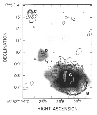
Figure 5: The Southern radio lobe (the Northern one is denoted by C) of the quasar MG 1654+134 ($z=1.7$, central component Q coincident with the optical QSO position), shown here as contours, is mapped into a complete Einstein ring by a foreground galaxy (G), indicated by the grayscale image. For this lens system, probably the most datailed mass analysis was performed – see text (image is from Langston et al. 1990)

Modeling of strong lens systems which contain Einstein rings yield much better constrained lens parameters and therefore even more accurate mass estimates; a beautiful example of this is the radio ring MG1645+134 (see Kochanek 1995; Wallington et al. 1996) around a foreground elliptical galaxy at $z=0.25$ shown in Fig. 5.

Results from fitting parametrized mass models to observed multiple image systems include the following: Many lens systems require quite a strong external shear, which may be explained by massive ellipticals being preferentially located in dense regions, i.e. in clusters or groups. The orientation of the mass ellipticity follows closely that of light distribution; however, this is not the case for the magnitude of ellipticity (Keeton et al. 1998). From mass modelling and detailed spectroscopic studies of lens galaxies, the latter in combination with stellar dynamical arguments, one finds that inside the Einstein radius, about half the mass is dark, and half is baryonic (Treu & Koopmans 2002; Koopmans & Treu 2003); therefore, in massive (lens) galaxies, baryons have strongly affected the mass profile, owing to their cooling and contraction. These authors have also shown that over the radius relevant for lensing, the profile is very well approximated by an isothermal one.

This issue is closely related to the determination of the Hubble constant from measuring time delays in multiple image systems. At present, time delays are known for about 10 lens systems, in some cases with an accuracy of 1%. Therefore, $H_{0}$ can in principle be obtained by (2.19). However, reality turns out to be considerably more difficult. The major difficulty lies in the so-called mass-sheet degeneracy, which says that the transformation $\kappa({\hbox{$\bf\theta$}})\to\lambda\kappa({\hbox{$\bf\theta$}})+(1-\lambda)$ of the surface mass density leaves the image positions and magnification ratios invariant, but changes the time delay by a factor $\lambda$ (Falco et al. 1985). Essentially, the bracket in (2.19) depends on the mean surface mass density within the annular region around the lens in which the multiple images are located (Kochanek 2002), and the mass-sheet degeneracy changes that value. One therefore requires additional information about the mass profile in galaxies.

As mentioned above, an isothermal profile ($\kappa\propto\theta^{-1}$) provides a reasonable fit to lens systems. Assuming an isothermal profile yields values of the Hubble constant of order $H_{0}\approx 50\,{\rm km/s/Mpc}$, consistently for the ‘simple’ lens systems. This is at variance with the value $H_{0}\approx 72\,{\rm km/s/Mpc}$ obtained from the Hubble Key Project (Freedman et al. 2001). On the other hand, the isothermal profile is at best a reasonable approximation to the real mass profile. Cosmological simulations yield a cuspy profile, such as the one found by Navarro et al. (1997; herafter NFW). These dark matter profiles are then modified by baryons cooling inside these halos; the larger the baryon fraction, the more are the dark matter profiles affected. Kochanek (2003) pointed out that in order to get a value of $H_{0}$ from lensing which is compatible with that from the Hubble Key Project, one would need a baryon fraction as large as $20\%$ of the total dark matter in the halo to cool, in order to render the central mass profiles of lenses steep enough; in effect, that leads to constant M/L-models within the region where the multiple images are found. This high fraction of cold baryons in galaxies is at odds with the local inventories of baryonic mass in galaxies. At present, the origin of this discrepancy is not known.

3.3 Substructure in lens galaxies

Whereas ‘simple’ lens models can usually fit the image positions very well, in most lens systems they are unable to provide a good fit to the flux ratios. The best known (but by far not worst) case is QSO 1422+231, where several groups have tried, and failed, to obtain a good lens model explaining image positions and fluxes. Mao & Schneider (1998) have provided an analytical argument, based on the universality of the lens mapping near cusps, why one would not expect to find a smooth model for this system. Since the flux ratios in this system are most reliably and accurately measured in the radio, absorption by the ISM in the (elliptical) lens galaxy is expected to be negligible. We argued that small-scale structure in the mass distribution can change the magnification, but leave the image position essentially unchanged; this is due to the fact that the deflection angle depends on first partial derivatives of the deflection potential $\psi$, whereas the magnification depends on $\kappa$ and $\gamma$, and thus on second derivatives of $\psi$; those are more strongly affected by small-scale structure.

This effect has been known for a long time: the optical and UV radiation from QSOs comes from a region small enough that even stars in the lens galaxy can affect their magnification, whereas the corresponding deflections are of order $10^{-6}$ arcseconds – this microlensing phenomenon (see, e.g., Wambsganss et al. 1990) shows up as uncorrelated brightness variations in the multiple images, and has clearly been detected in the QSO 2237+0305 (Schmidt et al. 2002) and in some of the other lens systems. However, the VLBI images of QSO 1422+231 are extended, and therefore individual stars cannot affect their magnification. But massive structures with $M\mathrel{\mathchoice{\lower 2.0pt\vbox{\halign{$\m@th\displaystyle\hfil#\hfil$\cr>\crcr\sim\crcr}}}{\lower 2.0pt\vbox{\halign{$\m@th\textstyle\hfil#\hfil$\cr>\crcr\sim\crcr}}}{\lower 2.0pt\vbox{\halign{$\m@th\scriptstyle\hfil#\hfil$\cr>\crcr\sim\crcr}}}{\lower 2.0pt\vbox{\halign{$\m@th\scriptscriptstyle\hfil#\hfil$\cr>\crcr\sim\crcr}}}}10^{7}M_{\odot}$ can change their magnification. Recall that CDM models of structure formation actually predict the presence of sub-halos in each massive galaxy – the (missing, since unobserved) satellites. As shown by Dalal & Kochanek (2002; and references therein), the statistics of mismatches between observed flux ratios and those predicted by simple lens models which fit the image positions in 4-image systems is in agreement with expectations from CDM satellites. Bradac et al. (2002) have explicitly demonstrated that the flux ratio problem in QSO 1422+231 is cured by placing a low-mass halo near one of the QSO images. Kochanek & Dalal (2003) have considered, and ruled out, alternative explanations for the flux ratio mismatches, such as interstellar scattering. One of the signatures of mass substructure, first found in investigations of microlensing (Schechter & Wambsganss 2002), is that the brightest saddle point is expected to be affected most, in the sense that it has a high probability of being substantially demagnified. Kochanek & Dalal have shown that this particular behavior is seen in a sample of 7 quadruple image lens systems. This behavior cannot be explained by absorption, scattering or scintillation by the interstellar medium of the lens galaxy. Hence, lensing has probably detected the ‘missing’ satellites in galaxy halos; the observed flux mismatches require a mass fraction in subclumps of order a few percent of the total lens mass, in accordance with predictions from CDM simulations. Bradac et al. (2002, 2003) have generated synthetic lens systems, using model galaxies as obtained from CDM simulations as deflectors, and have shown that the resulting image fluxes are at variance with the predictions from simple lens models, again due to the substructure in the mass distribution. In a few of the observed lens systems, a fairly massive subclump can be identified directly by its luminosity, yielding further support to this interpretation.

3.4 Other properties of lens galaxies

3.4.1 Evolution

Early-type galaxies are known to be located on the so-called fundamental plane (FP), i.e., there is a relation between their central surface brightness, their effective radius and the velocity dispersion in these galaxies. The FP has been observed even to high redshifts, using early-type galaxies in high-redshift clusters; it is known to evolve with $z$, mainly due to passive evolution of the stellar population. The lens galaxies form a mass-selected sample of galaxies not selected for cluster membership, and it is therefore of great interest to see whether they also obey a FP relation. In fact, since lens galaxies have a well-determined mass scale (or $\sigma_{v}$, after fitting an isothermal mass model), and are spread over a large redshift range, they are ideal for FP research. Rusin et al. (2003) have found from a sample of 28 lenses that the evolution of the FP is compatible with passive stellar evolution, and that it favours a high redshift for the epoch of star formation in these galaxies.

3.4.2 The interstellar matter in lens galaxies

Multiple image systems provide us with views of the same source along different lines-of-sight. Excluding time-delay effects in connection with spectral variability, as well as differential magnification, spectral differences between the images can then only be caused by propagation effects. In particular, one can study the properties of the dust in lens galaxies, as color differences between images can be attributed to different extinction and reddening along the different lines-of-sight through the lens galaxy. Falco et al. (1999) have investigated 23 gravitational lens galaxies over the range $0\mathrel{\mathchoice{\lower 2.0pt\vbox{\halign{$\m@th\displaystyle\hfil#\hfil$\cr<\crcr\sim\crcr}}}{\lower 2.0pt\vbox{\halign{$\m@th\textstyle\hfil#\hfil$\cr<\crcr\sim\crcr}}}{\lower 2.0pt\vbox{\halign{$\m@th\scriptstyle\hfil#\hfil$\cr<\crcr\sim\crcr}}}{\lower 2.0pt\vbox{\halign{$\m@th\scriptscriptstyle\hfil#\hfil$\cr<\crcr\sim\crcr}}}}z_{\rm d}\mathrel{\mathchoice{\lower 2.0pt\vbox{\halign{$\m@th\displaystyle\hfil#\hfil$\cr<\crcr\sim\crcr}}}{\lower 2.0pt\vbox{\halign{$\m@th\textstyle\hfil#\hfil$\cr<\crcr\sim\crcr}}}{\lower 2.0pt\vbox{\halign{$\m@th\scriptstyle\hfil#\hfil$\cr<\crcr\sim\crcr}}}{\lower 2.0pt\vbox{\halign{$\m@th\scriptscriptstyle\hfil#\hfil$\cr<\crcr\sim\crcr}}}}1$. Given that most lens galaxies are early types, they found a small median differential extinction of $\Delta E(B-V)\sim 0.05$, with slightly larger (smaller) values for radio- (optically-)selected lens systems. The lack of a clear correlation with the separation of the image from the lens center points towards patchy extinction. Two spiral lens galaxies show a substantially larger extinction. The extinction law, i.e., the relation between extinction and reddening, varies between different lens galaxies over quite some range; the Galactic extinction law is therefore by no means universally applicable.

4 Weak gravitational lensing

Multiple images, microlensing (with appreciable magnifications) and arcs in clusters are phenomena of strong lensing. In weak gravitational lensing, the Jacobi matrix ${\cal A}$ is very close to the unit matrix, which implies weak distortions and small magnifications. Those cannot be identified in individual sources, but only in a statistical sense; the basics of these effects will be described in this section, and several applications will be dicussed in later sections.

4.1 Distortion of faint galaxy images

Images of distant, extended sources are distorted in shape and size; this is described by the locally linearized lens equation around the image center ${\hbox{$\bf\theta$}}_{0}$,

$${\hbox{$\bf\beta$}}-{\hbox{$\bf\beta$}}_{0}={\mathcal{A}}({\hbox{$\bf\theta$}}_{0})\cdot({\hbox{$\bf\theta$}}-{\hbox{$\bf\theta$}}_{0})\;,$$ (4.1)

where ${\hbox{$\bf\beta$}}_{0}={\hbox{$\bf\beta$}}({\hbox{$\bf\theta$}}_{0})$, with the Jacobian (2.18), and the invariance of surface brightness (2.16). Recall that the shape distortion is described by the (reduced) shear which is a two-component quantity, most conveniently written as a complex number,

$$\gamma=\gamma_{1}+{\rm i}\gamma_{2}=|\gamma|\,{\rm e}^{2{\rm i}\varphi}\;;\quad g=g_{1}+{\rm i}g_{2}=|g|\,{\rm e}^{2{\rm i}\varphi}\;;$$ (4.2)

its amplitude describes the degree of distortion, whereas its phase $\varphi$ yields the direction of distortion. The reason for the factor ‘2’ in the phase is the fact that an ellipse transforms into itself after a rotation by $180^{\circ}$. Consider a circular source with radius $r$; mapped by the local Jacobi matrix, its image is an ellipse, with semi-axes

$${r\over 1-\kappa-|\gamma|}={r\over(1-\kappa)(1-|g|)}\quad;\quad{r\over 1-\kappa+|\gamma|}={r\over(1-\kappa)(1+|g|)}\;$$

and the major axis encloses an angle $\varphi$ with the positive $\theta_{1}$-axis. Hence, if circular sources could be identified, the measured image ellipticities would immediately yield the value of the reduced shear, through the axis ratio

$$|g|={1-b/a\over 1+b/a}\quad\Leftrightarrow\quad{b\over a}={1-|g|\over 1+|g|}$$

and the orientation of the major axis $\varphi$. However, faint galaxies are not intrinsically round, so that the observed image ellipticity is a combination of intrinsic ellipticity and shear. The strategy to nevertheless obtain an estimate of the (reduced) shear consists in locally averaging over many galaxy images, assuming that the intrinsic ellipticities are randomly oriented. In order to follow this strategy, one needs to clarify first how to define ‘ellipticity’ for a source with arbitrary isophotes (faint galaxies are not simply elliptical); in addition, seeing caused by atmospheric turbulence will blur – and thus circularize – observed images. We will consider these issues in turn.

4.2 Measurements of shapes and shear

Let $I({\hbox{$\bf\theta$}})$ be the brightness distribution of an image, assumed to be isolated on the sky; the center of the image can be defined as

$$\bar{{\hbox{$\bf\theta$}}}\equiv\frac{\int\!{\rm d}^{2}\theta\,q_{I}[I({\hbox{$\bf\theta$}})]\,{\hbox{$\bf\theta$}}}{\int\!{\rm d}^{2}\theta\,q_{I}[I({\hbox{$\bf\theta$}})]}\;,$$ (4.3)

where $q_{I}(I)$ is a suitably chosen weight function; e.g., if $q_{I}(I)=I\,{\rm H}(I-I_{\rm th})$, $\bar{{\hbox{$\bf\theta$}}}$ would be the center of light within a limiting isophote of the image (where H denotes the Heaviside step function). We next define the tensor of second brightness moments,

$$Q_{ij}=\frac{\int\!{\rm d}^{2}\theta\,q_{I}[I({\hbox{$\bf\theta$}})]\,(\theta_{i}-\bar{\theta}_{i})\,(\theta_{j}-\bar{\theta}_{j})}{\int\!{\rm d}^{2}\theta\,q_{I}[I({\hbox{$\bf\theta$}})]}\;,\quad i,j\in\{1,2\}\;.$$ (4.4)

Note that for an image with circular isophotes, $Q_{11}=Q_{22}$, and $Q_{12}=0$. The trace of $Q$ describes the size of the image, whereas the traceless part of $Q_{ij}$ contains the ellipticity information.

From $Q_{ij}$, one defines two complex ellipticities,

$$\framebox{$\displaystyle\chi\equiv\frac{Q_{11}-Q_{22}+2{\rm i}Q_{12}}{Q_{11}+Q_{22}}$}\;\;\;{\rm and}\;\;\framebox{$\displaystyle\epsilon\equiv\frac{Q_{11}-Q_{22}+2{\rm i}Q_{12}}{Q_{11}+Q_{22}+2(Q_{11}Q_{22}-Q_{12}^{2})^{1/2}}$}\;.$$ (4.5)

Both of them have the same phase (because of the same numerator), but a different absolute value; for an image with elliptical isophotes of axis ratio $r\leq 1$, one obtains

$$|\chi|={1-r^{2}\over 1+r^{2}}\quad;\quad|{\epsilon}|={1-r\over 1+r}\;.$$ (4.6)

Which of these two definitions is more convenient depends on the context; one can easily transform one into the other,

$$\epsilon=\frac{\chi}{1+(1-|\chi|^{2})^{1/2}}\;,\quad\chi=\frac{2\epsilon}{1+|\epsilon|^{2}}\;.$$ (4.7)

4.2.1 From source to image ellipticities

In total analogy, one defines the second-order brightness tensor $Q^{(\rm s)}_{ij}$, and the complex ellipticities $\chi^{(\rm s)}$ and $\epsilon^{(\rm s)}$ for the unlensed source. From

$$Q^{(\rm s)}_{ij}=\frac{\int\!{\rm d}^{2}\beta\,q_{I}[I^{(\rm s)}({\hbox{$\bf\beta$}})]\,(\beta_{i}-\bar{\beta}_{i})\,(\beta_{j}-\bar{\beta}_{j})}{\int\!{\rm d}^{2}\beta\,q_{I}[I^{(\rm s)}({\hbox{$\bf\beta$}})]}\;,\quad i,j\in\{1,2\}\;,$$ (4.8)

one finds with ${\rm d}^{2}\beta=\det{\cal A}\,{\rm d}^{2}\theta$, ${\hbox{$\bf\beta$}}-\bar{{\hbox{$\bf\beta$}}}={\cal A}\left({\hbox{$\bf\theta$}}-\bar{{\hbox{$\bf\theta$}}}\right)$ that

$$Q^{(\rm s)}={\cal A}\,Q\,{\cal A}^{T}={\cal A}\,Q\,{\cal A}\;,$$ (4.9)

where ${\cal A}\equiv{\cal A}(\bar{{\hbox{$\bf\theta$}}})$ is the Jacobi matrix of the lens equation at position $\bar{{\hbox{$\bf\theta$}}}$. Using the definitions of the complex ellipticities, one finds the transformations:

$$\framebox{$\displaystyle\chi^{(\rm s)}=\frac{\chi-2g+g^{2}\chi^{*}}{1+|g|^{2}-2{\cal R}\hbox{e}(g\chi^{*})}$}\;;\quad\framebox{$\displaystyle\epsilon^{(\rm s)}=\left\{\begin{array}[]{ll}\displaystyle\frac{\epsilon-g}{1-g^{*}\epsilon}&\quad\hbox{if}\;|g|\leq 1\;;\\ \\ \displaystyle\frac{1-g\epsilon^{*}}{\epsilon^{*}-g^{*}}&\quad\hbox{if}\;|g|>1\;.\\ \end{array}\right.$}$$ (4.10)

The inverse transformations are obtained by interchanging source and image ellipticities, and $g\to-g$ in the foregoing equations.

4.2.2 Estimating the (reduced) shear

In the following we make the assumption that the intrinsic orientation of galaxies is random,

$$\mathrm{E}\left(\chi^{(\rm s)}\right)=0=\mathrm{E}\left(\epsilon^{(\rm s)}\right)\;,$$ (4.11)

which is expected to be valid since there should be no direction singled out in the Universe. This then implies that the expectation value of ${\epsilon}$ is [as obtained by averaging the transformation law (4.10) over the phase of the intrinsic source orientation (Schramm & Kaiser 1995; Seitz & Schneider 1997)]

$$\framebox{$\displaystyle{\rm E}(\epsilon)=\left\{\begin{array}[]{ll}\displaystyle g&\quad\hbox{if}\;|g|\leq 1\\ \\ \displaystyle 1/g^{*}&\quad\hbox{if}\;|g|>1\;.\\ \end{array}\right.$}$$ (4.12)

This is a remarkable result, since it shows that each image ellipticity provides an unbiased estimate of the local shear, though a very noisy one. The noise is determined by the intrinsic ellipticity dispersion

$$\sigma_{\epsilon}=\sqrt{\left\langle{\epsilon}^{(\rm s)}{\epsilon}^{(\rm s)*}\right\rangle}\;.$$

This noise can be beaten down by averaging over many galaxy images. Fortunately, we live in a Universe where the sky is ‘full of faint galaxies’, as was impressively demonstrated by the Hubble Deep Field images (Williams et al. 1996). Hence, the accuracy of a shear estimate depends on the local number density of galaxies for which a shape can be measured. In order to obtain a high density, one requires deep imaging observations. As a rough guide, on a 3 hour exposure under excellent observing conditions with a 3-meter class telescope, about 30 galaxies per arcmin² can be used for a shape measurement.

Note that in the weak lensing regime, $\kappa\ll 1$, $|\gamma|\ll 1$, one finds

$$\gamma\approx g\approx\langle\epsilon\rangle\approx\frac{\langle\chi\rangle}{2}\;.$$ (4.13)

4.3 Problems in measuring shear, and their solutions

4.3.1 Major problems

• Seeing, that is the finite size of the point spread function (PSF), circularizes images; this effect is severe since faint galaxies (i.e. those at a magnitude limit for which the number density is of order 30 per arcmin²) are not larger than the typical seeing disk. Therefore, weak lensing requires imaging with very good seeing.

• The PSF is not circular, owing to e.g., wind shake of the telescope, or tracking errors. However, an anisotropic PSF causes round sources to appear elliptical, and thus mimics shear.

• Galaxy images are not isolated, and therefore the integrals in the definition of $Q_{ij}$ have to be cut-off at a finite radius. Hence, one usually uses a weight function $q$ which depends explicitly on $|{\hbox{$\bf\theta$}}-\bar{\hbox{$\bf\theta$}}|$; however, this modifies the transformation (4.10) between image and source ellipticity.

• The sky noise, i.e. the finite brightness of the night sky, introduces a noise component in the measurement of image ellipticities from CCD data, so that only for high-S/N objects can a shape be measured.

• Distortion by telescope and camera optics renders the coaddition of exposures complex; one needs to employ remapping, using accurate astrometry, and sub-pixel coaddition.

Depending on the science application, the shear one wants to measure is of order a few percent, or even smaller. Essentially all of the effects mentioned can introduce ellipticities of the same order in the measured images if they are not carefully taken into account.

4.3.2 Solutions

In order to deal with these issues, specific software has been developed. The one that has been mostly used up to now is the Kaiser et al. (1995, KSB) method, or its implementation IMCAT. Its basic idea is as follows: the image ellipticity will be determined by the intrinsic ellipticity, the (reduced) shear, the size of the PSF and its anisotropy. Note that the PSF can be investigated by identifying stars (that is: point sources) on the images. The response of $\chi$ to the shear depends on the size of the source – for small sources, blurring by seeing reduces the response to a large degree. The size of the sources is estimated from the size of the seeing-convolved images. In addition, the response of $\chi$ to a PSF anisotropy also depends on the image size. The KSB method, an essential part of which was put forward by Luppino & Kaiser (1997; for a complete derivation, see Sect. 4.6.2 of Bartelmann & Schneider 2001), results in the relation

$$\framebox{$\displaystyle\chi^{\rm obs}_{\alpha}=\hat{\chi}^{0}_{\alpha}+P^{\rm sm}_{\alpha\beta}q_{\beta}+P^{g}_{\alpha\beta}g_{\beta}$}\;,$$ (4.14)

where $\hat{\chi}^{0}$ is the ellipticity of the source convolved with the isotropic part of the PSF and therefore, its expectation value vanishes, according to the assumption of randomly oriented sources, ${\rm E}(\hat{\chi}^{0})=0$. The tensor $P^{\rm sm}_{\alpha\beta}$ describes the response of the image ellipticity to the PSF anisotropy, which is quantified by the (complex) ellipticity $q_{\beta}$ of the PSF, as measured from stars. $P^{g}_{\alpha\beta}$ is a tensor which describes the response of the image ellipticity to an applied shear. Both, $P^{\rm sm}_{\alpha\beta}$ and $P^{g}_{\alpha\beta}$ are calculated for each image individually; they depend on higher-order moments of the image brightness distribution and the size of the PSF. Detailed simulations (e.g., Erben et al. 2001; Bacon et al. 2001) have shown that the KSB method can measure shear with better than $\sim 10\%$ accuracy. Several other methods for measuring image shapes in order to obtain an estimate of the local shear have been developed and some of them have already been applied to observational data (Bonnet & Mellier 1995; Kuijken 1999; Kaiser 2000; Bernstein & Jarvis 2002; Refregier & Bacon 2003).

4.4 Magnification effects

The magnification caused by the differential light bending changes the apparent brightness of sources; this leads to two effects:

1. The observed flux $S$ from a source is changed from its unlensed value $S_{0}$ according to $S=\mu\,S_{0}$; if $\mu>1$, sources appear brighter than they would without an intervening lens.

2. A population of sources in the unlensed solid angle $\omega_{0}$ is spread over the solid angle $\omega=\mu\omega_{0}$ due to the magnification.

These two effects affect the number counts of sources differently; which one of them wins depends on the slope of the number counts; one finds

$$\framebox{$\displaystyle n(>S,{\hbox{$\bf\theta$}},z)=\frac{1}{\mu({\hbox{$\bf\theta$}},z)}\,n_{0}\left(>\frac{S}{\mu({\hbox{$\bf\theta$}},z)},z\right)$}\;,$$ (4.15)

where $n(>S,z)$ and $n_{0}(>S,z)$ are the lensed and unlensed cumulative number counts of sources, respectively. The first argument of $n_{0}$ accounts for the change of the flux, whereas the prefactor in (4.15) stems from the change of apparent solid angle.

As an illustrative example, we consider the case that the source counts follow a power law,

$$n_{0}(>S)=a\,S^{-\alpha}\;;$$ (4.16)

one then finds for the lensed counts in a region of the sky with magnification $\mu$:

$$\frac{n(>S)}{n_{0}(>S)}=\mu^{\alpha-1}\;,$$ (4.17)

and therefore, if $\alpha>1$ ($<1$), source counts are enhanced (depleted); the steeper the counts, the stronger the effect. In the case of weak lensing, where $|\mu-1|\ll 1$, one probes the source counts only over a small range in flux, so that they can always be approximated (locally) by a power law.

One important example is provided by the lensing of QSOs. The QSO number counts are steep at the bright end, and flat for fainter sources. This implies that in regions of magnification $>1$, bright QSO should be overdense, faint ones underdense. This magnification bias is the reason why the fraction of lensed sources is much higher in bright QSO samples than in fainter ones!

4.5 Tangential and cross component of shear

4.5.1 The shear components

The shear components $\gamma_{1}$ and $\gamma_{2}$ are defined relative to a reference Cartesian coordinate frame. Note that the shear is not a vector, owing to its transformation properties under rotations, which is the same as that of the linear polarization; it is therefore called a polar. In analogy with vectors, it is often useful to consider the shear components in a rotated reference frame, that is, to measure them w.r.t. a different direction; for example, the arcs in clusters are tangentially aligned, and so their ellipticity is oriented approximately tangent to the radius vector in the cluster.

If $\phi$ specifies a direction, one defines the tangential and cross components of the shear relative to this direction as

$$\framebox{$\displaystyle\gamma_{\rm t}=-{\cal R}\hbox{e}\left[\gamma\,{\rm e}^{-2{\rm i}\phi}\right]\quad,\quad\gamma_{\times}=-{\cal I}\hbox{m}\left[\gamma\,{\rm e}^{-2{\rm i}\phi}\right]$}\;.$$ (4.18)

For example, in the case of a circularly-symmetric matter distribution, the shear at any point will be oriented tangent to the direction towards the center of symmetry. Thus in this case, choose $\phi$ to be the polar angle of a point; then, $\gamma_{\times}=0$. In full analogy to the shear, one defines the tangential and cross components of an image ellipticity, ${\epsilon}_{\rm t}$ and ${\epsilon}_{\times}$.

4.5.2 Minimum lens strength for its weak lensing detection

As a first application of this decomposition, we consider how massive a lens needs to be in order to produce a detectable weak lensing signal. For this purpose, consider a lens modeled as an SIS with one-dimensional velocity dispersion $\sigma_{v}$. In the annulus $\theta_{\rm in}\leq\theta\leq\theta_{\rm out}$, centered on the lens, let there be $N=n\pi(\theta_{\rm out}^{2}-\theta_{\rm in}^{2})$ galaxy images with position ${\hbox{$\bf\theta$}}_{i}=\theta_{i}(\cos\phi_{i},\sin\phi_{i})$ and (complex) ellipticities ${\epsilon}_{i}$. For each one of them, consider the tangential ellipticity

$${\epsilon}_{{\rm t}i}=-{\cal R}\hbox{e}\left({\epsilon}_{i}\,{\rm e}^{-2{\rm i}\phi_{i}}\right)\;.$$ (4.19)

Next we define a statistical quantity to measure the degree of tangential alignment of the galaxy images, and thus the lens strength:

$$X\equiv\sum_{i=1}^{N}a_{i}\,\epsilon_{{\rm t}i}\;,$$ (4.20)

where the factors $a_{i}=a(\theta_{i})$ are arbitrary at this point, and will later be chosen such as to maximize the signal-to-noise ratio of this estimator. The shear of an SIS is given by

$$\gamma_{\rm t}(\theta)={\theta_{\rm E}\over 2\theta}=2\pi\left(\sigma_{v}\over c\right)^{2}\left(D_{\rm ds}\over D_{\rm s}\right)\,{1\over\theta}\;.$$ (4.21)

The expectation value of the ellipticity is ${\rm E}(\epsilon_{{\rm t}i})=\gamma_{\rm t}(\theta_{i})$, so that ${\rm E}(X)=\theta_{\rm E}\sum_{i}a_{i}/(2\theta_{i})$. Since $\epsilon_{{\rm t}i}=\epsilon_{{\rm t}i}^{(\rm s)}+\gamma_{{\rm t}}(\theta_{i})$ in the weak lensing regime, one has ${\rm E}(\epsilon_{{\rm t}i}\epsilon_{{\rm t}j})=\gamma_{{\rm t}}(\theta_{i})\gamma_{{\rm t}}(\theta_{j})+\delta_{ij}\sigma_{\epsilon}^{2}/2$, thus

$${\rm E}(X^{2})=\sum_{i,j=1}^{N}a_{i}a_{j}\,{\rm E}(\epsilon_{{\rm t}i}\epsilon_{{\rm t}j})=[{\rm E}(X)]^{2}+\frac{\sigma_{\epsilon}^{2}}{2}\sum_{i=1}^{N}a_{i}^{2}\;.$$ (4.22)

Therefore, the signal-to-noise ratio for a detection of the lens is

$$\frac{{\rm S}}{{\rm N}}=\frac{\theta_{\rm E}}{\sqrt{2}\sigma_{\epsilon}}\,\frac{\sum_{i}a_{i}\,\theta_{i}^{-1}}{\sqrt{\sum_{i}a_{i}^{2}}}\;.$$ (4.23)

The $a_{i}$ can now be chosen so as to maximize S/N; from differentiation of S/N, one finds a maximum if $a_{i}\propto 1/\theta_{i}$. Then, performing the ensemble average over the galaxy positions, one finally obtains:

$$\frac{{\rm S}}{{\rm N}} = \frac{\theta_{\rm E}}{\sigma_{\epsilon}}\,\sqrt{\pi n}\,\sqrt{\ln(\theta_{\rm out}/\theta_{\rm in})}$$

$$= 8.4\,\left(\frac{n}{30\,{\rm arcmin}^{-2}}\right)^{1/2}\left(\frac{\sigma_{\epsilon}}{0.3}\right)^{-1}\left(\frac{\sigma_{v}}{600\,{\rm km\,s}^{-1}}\right)^{2}$$

$$\times \phantom{8.4\,}\left(\frac{\ln(\theta_{\rm out}/\theta_{\rm in})}{\ln 10}\right)^{1/2}\left\langle\frac{D_{\rm ds}}{D_{\rm s}}\right\rangle\;.$$

From this consideration we conclude that clusters of galaxies with $\sigma_{v}\mathrel{\mathchoice{\lower 2.0pt\vbox{\halign{$\m@th\displaystyle\hfil#\hfil$\cr>\crcr\sim\crcr}}}{\lower 2.0pt\vbox{\halign{$\m@th\textstyle\hfil#\hfil$\cr>\crcr\sim\crcr}}}{\lower 2.0pt\vbox{\halign{$\m@th\scriptstyle\hfil#\hfil$\cr>\crcr\sim\crcr}}}{\lower 2.0pt\vbox{\halign{$\m@th\scriptscriptstyle\hfil#\hfil$\cr>\crcr\sim\crcr}}}}600\,{\rm km/s}$ can be detected with sufficiently large S/N by weak lensing, but individual galaxies ($\sigma_{v}\sim 200\,{\rm km/s}$) are too weak as lenses to be detected individually.

4.6 Galaxy-galaxy lensing

Whereas galaxies are not massive enough to show a weak lensing signal individually, the signal of many galaxies can be (statistically) superposed. Consider sets of foreground (lens) and background galaxies; on average, in a foreground-background galaxy pair, the ellipticity of the background galaxy will be oriented preferentially in the direction tangent to the connecting line. In other words, if $\varphi$ is the angle between the major axis of the background galaxy and the connecting line between foreground and background galaxy, values $\pi/4\leq\varphi\leq\pi/2$ should be slighly more frequent than $0\leq\varphi\leq\pi/4$. The mean tangential ellipticity $\left\langle{\epsilon}_{{\rm t}}(\theta)\right\rangle$ of background galaxies relative to the direction towards foreground galaxies measures the mean tangential shear at this separation.

The strength of this mean tangential shear measures mass properties of the galaxy population selected as potential lenses. In order to properly interpret the lensing signal, one needs to know the redshift distribution of the foreground and background galaxies. Furthermore, one needs to assume a relation between the lens galaxies’ luminosity and mass properties (such as a Faber–Jackson type of relation), unless the sample is so large that one can finely bin the galaxies with respect to their luminosities; this requires of course redshift information. In this way, the velocity dispersion $\sigma_{*}$ of an $L_{*}$-galaxy can be determined from galaxy-galaxy lensing. Furthermore, galaxy-galaxy lensing provides a highly valuable tool to study the mass distribution of galaxy halos at distances from their centers which are much larger than the extent of luminous tracers, such as stars and gas – or ask the question of where the galaxy halos ‘end’.

Whereas the first detection of galaxy-galaxy lensing (Brainerd et al. 1996) was based on a single field with $\sim 9^{\prime}$ sidelength, much larger surveys have now become available, most noticibly the SDSS (Fischer et al. 2000; McKay et al. 2001). These large data sets have allowed the splitting of the lens galaxies into subsamples and to investigate their properties separately. From this it was verified that early-type galaxies have a larger mass than spiral galaxies with the same luminosity, and that this behaviour extends to large radii. Furthermore, the lensing signal for early-type galaxies can be detected out to much larger scales than for late-types. The interpretation of this result is not unique: it either can mean that ellipticals have a more extended halo than spirals, or that the lens signal from ellipticals, which tend to be preferentially located inside groups and clusters, arises in fact from the host halo in which they reside (see also Guzik & Seljak 2002). Indeed, when the lens galaxy sample is divided into those living in high- and low-density environments, the former ones have a significantly more extended lensing signal.

What the galaxy-galaxy signal really measures is the relation between light (galaxies) and mass. In its simplest terms, this relation can be expressed by a bias factor $b$ and the correlation coefficient $r$. Schneider (1998) and van Waerbeke (1998) pointed out that lensing can be used to study the bias factor as a function of scale and redshift, by correlating the lensing signal with the number density of galaxies. In fact, as shown in Hoekstra et al. (2002b), both $b$ and $r$ can be expressed in terms of the galaxy-galaxy lensing signal, the angular correlation function of the (lens) galaxies and the cosmic shear signal (see Sect. 6 below). Applying this method to the combination of the Red-Sequence Cluster Survey and the VIRMOS-DESCART survey, they derived the scale dependence of $b$ and $r$; on large (linear) scales, their results are compatible with constant values, whereas on smaller scales it appears that both of these functions vary. Future surveys will allow much more detailed studies on the relation between mass and light, and therefore determine the biasing properties of galaxies from observations directly. This is of course of great interest, since the unknown behavior of the biasing yields the uncertainty in the transformation of the power spectrum of the galaxy distribution, as determined from extensive galaxy redshift surveys, to that of the underlying mass distribution. Hence, weak lensing is able to provide this crucial calibration.

5 Lensing by clusters of galaxies

5.1 Introduction

Clusters are the most massive bound structures in the Universe; this, together with the (related) fact that their dynamical time scale (e.g., the crossing time) is not much smaller than the Hubble time – so that they retain a ‘memory’ of their formation – render them of particular interest for cosmologists. The evolution of their abundance, i.e., their comoving number density as a function of mass and redshift, is an important probe for cosmological models. Furthermore, they form signposts of the dark matter distribution in the Universe. Clusters act as laboratories for studying the evolution of galaxies and baryons in the Universe. In fact, clusters were (arguably) the first objects for which the presence of dark matter has been concluded (by Zwicky in 1933).

5.2 The mass of galaxy clusters

Cosmologists can predict the abundance of clusters as a function of their mass (e.g., using numerical simulations); however, the mass of a cluster is not directly observable, but only its luminosity, or the temperature of the X-ray emitting intra-cluster medium. Therefore, in order to compare observed clusters with the cosmological predictions, one needs a way to determine their masses. Three principal methods for determining the mass of galaxy clusters are in use:

• Assuming virial equilibrium, the observed velocity distribution of galaxies in clusters can be converted into a mass estimate; this method typically requires assumptions about the statistical distribution of the anisotropy of the galaxy orbits.

• The hot intra-cluster gas, as visible through its Bremsstrahlung in X-rays, traces the gravitational potential of the cluster. Under certain assumptions (see below), the mass profile can be constructed from the X-ray emission.

• Weak and strong gravitational lensing probe the projected mass profile of clusters; this will be described further below.

All three methods are complementary; lensing yields the line-of-sight projected density of clusters, in contrast to the other two methods which probes the mass inside spheres. On the other hand, those rely on equilibrium (and symmetry) conditions.

5.2.1 X-ray mass determination of clusters

The intracluster gas emits via Bremsstrahlung; the emissivity depends on the gas density and temperature, and, at lower $T$, on its chemical composition. Assuming that the gas is in hydrostatic equilibrium in the potential well of cluster, the gas pressure $P$ must balance gravity, or

$$\nabla P=-\rho_{\rm g}\,\nabla\Phi\;,$$

where $\Phi$ is the gravitational potential and $\rho_{\rm g}$ is the gas density. In the case of spherical symmetry, this becomes

$${1\over\rho_{\rm g}}\,{{\rm d}P\over{\rm d}r}=-{{\rm d}\Phi\over{\rm d}r}=-{G\,M(r)\over r^{2}}\;.$$

From the X-ray brightness profile and temperature measurement, $M(r)$, the total mass inside $r$ (dark plus luminous) can then be determined,

$$\framebox{$\displaystyle M(r)=-{{k_{\rm B}}Tr^{2}\over G\mu m_{\rm p}}\left({{\rm d}\ln\rho_{\rm g}\over{\rm d}r}+{{\rm d}\ln T\over{\rm d}r}\right)$}\;.$$ (5.1)

However, the two major X-ray satellites currently operating, Chandra & XMM-Newton, have revealed that at least the inner regions of clusters show a considerably more complicated structure than implied by hydrostatic equilibrium. In some cases, the intracluster medium is obviously affected by a central AGN, which produces additional energy and entropy input. Cold fronts, with very sharp edges, and shocks have been discovered, most likely showing ongoing merger events. The temperature and metallicity appear to be strongly varying functions of position. Therefore, mass estimates of central parts of clusters from X-ray observations require special care.

5.3 Luminous arcs & multiple images

Strong lensing effects in clusters show up in the form of giant luminous arcs, strongly distorted arclets, and multiple images of background galaxies. Since strong lensing occurs only in the central part of clusters (typically corresponding to $\sim 50h^{-1}\,{\rm kpc}$), it can be used to probe only their inner mass structure. However, strong lensing yields by far the most accurate central mass determinations; in some favourable cases with many strong lensing features (such as for Abell 2218; see Fig. 2), accuracies better than $\sim 10\%$ can be achieved.

5.3.1 First go: $M(\leq\theta_{\rm E})$

Giant arcs occur where the distortion (and magnification) is very large, that is near critical curves. To a first approximation, assuming a spherical mass distribution, the location of the arc relative to the cluster center (which usually is assumed to coincide with the brightest cluster galaxy) yields the Einstein radius of the cluster, so that the mass estimate (3.1) can be applied. Therefore, this simple estimate yields the mass inside the arc radius. However, this estimate is not very accurate, perhaps good to within $\sim 50\%$. Its reliability depends on the level of asymmetry and substructure in the cluster mass distribution (Bartelmann 1995). Furthermore, it is likely to overestimate the mass in the mean, since arcs preferentially occur along the major axis of clusters. Of course, the method is very difficult to apply if the center of the cluster is not readily identified or if it is obviously bimodal. For these reasons, this simple method for mass estimates is not regarded as particularly accurate.

5.3.2 Detailed modelling

The mass determination in cluster centers becomes much more accurate if several arcs and/or multiple images are present, since in this case, detailed modelling can be done. This typically proceeds in an interactive way: First, multiple images have to be identified (based on their colors and/or detailed morphology, as available with HST imaging). Simple (plausible) mass models are then assumed, with parameters fixed by matching the multiple images, and requiring the distortion at the arc location(s) to be strong and have the correct orientation. This model then predicts the presence of further multiple images; they can be checked for through morphology and color. If confirmed, a new, refined model is constructed, which yields further strong lensing predictions etc. Such models have predictive power and can be trusted in quite some detail; the accuracy of mass estimates in some favourable cases can be as high as a few percent.

In fact, these models can be used to predict the redshift of arcs and arclets (Kneib et al. 1994): since the distortion of a lens depends on the source redshift, once a detailed mass model is available, one can estimate the value of the lens strength $\propto D_{\rm ds}/D_{\rm s}$ and thus infer the redshift. This method has been successfully applied to HST observations of clusters (Ebbels et al. 1998). Of course, having spectroscopic redshifts of the arcs available increases the accuracy of the calibration of the mass models; they are therefore very useful.

5.3.3 Results

The main results of the strong lensing investigations of clusters can be summarized as follows:

• The mass in cluster centers is much more concentrated than predicted by (simple) models based on X-ray observations. The latter usually predict a relatively large core of the mass distribution. These large cores would render clusters sub-critical to lensing, i.e., they would be unable to produce giant arcs or multiple images. In fact, when arcs were first discovered they came as a big surprise because of these expectations. By now we know that the intracluster medium is much more complicated than assumed in these ‘$\beta$-model’ fits for the X-ray emission.

• The mass distribution in the inner part of clusters often shows strong substructure, or multiple mass peaks. These are also seen in the galaxy distribution of clusters, but with the arcs can be verified to also correspond to mass peaks. These are easily understood in the frame of hierarchical mergers in a CDM model; the merged clusters retain their multiple peaks for a dynamical time or even longer, and are therefore not in virial equilibrium.

• The orientation of the (dark) matter appears to be fairly strongly correlated with the orientation of the light in the cD galaxy; this supports the idea that the growth of the cD galaxy is related to the cluster as a whole, through repeated accretion of lower-mass member galaxies. In that case, the cD galaxy ‘knows’ the orientation of the cluster.

• There is in general good agreement between lensing and X-ray mass estimates for those clusters where a ‘cooling flow’ indicates that they are in dynamical equilibrium, provided the X-ray analysis takes the presence of the cooling flow into account.

5.4 Mass reconstructions from weak lensing

Whereas strong lensing probes the mass distribution in the inner part of clusters, weak lensing can be used to study the mass distribution at much larger angular separations from the cluster center. In fact, as we shall see, weak lensing can provide a parameter-free reconstruction of the projected two-dimensional mass distribution in clusters. This discovery (Kaiser & Squires 1993) actually marked the beginning of quantitative weak lensing research.

5.4.1 The Kaiser–Squires inversion

Weak lensing yields an estimate of the local (reduced) shear, as discussed in Sect. 4.2. Here we shall discuss how to derive the surface mass density from a measurement of the (reduced) shear. Starting from (2.9) and the definition (2.15) of the shear, one finds that the latter can be written in the form

$$\gamma({\hbox{$\bf\theta$}}) = \frac{1}{\pi}\int_{{\rm I\mathchoice{\kern-1.99168pt}{\kern-1.99168pt}{\kern-1.84941pt}{\kern-1.42262pt}R}^{2}}{\rm d}^{2}\theta^{\prime}\,{\mathcal{D}}({\hbox{$\bf\theta$}}-{\hbox{$\bf\theta$}}^{\prime})\,\kappa({\hbox{$\bf\theta$}}^{\prime})\;,\quad\hbox{with}$$

$${\mathcal{D}}({\hbox{$\bf\theta$}}) \equiv \frac{\theta_{2}^{2}-\theta_{1}^{2}-2{\rm i}\theta_{1}\theta_{2}}{|{\hbox{$\bf\theta$}}|^{4}}=\frac{-1}{(\theta_{1}-{\rm i}\theta_{2})^{2}}\;.$$ (5.2)

Hence, the complex shear $\gamma$ is a convolution of $\kappa$ with the kernel ${\cal D}$, or, in other words, ${\cal D}$ describes the shear generated by a point mass. In Fourier space this convolution becomes a multiplication,

$$\hat{\gamma}({\hbox{$\bf\ell$}})=\pi^{-1}\hat{\mathcal{D}}({\hbox{$\bf\ell$}})\,\hat{\kappa}({\hbox{$\bf\ell$}})\quad{\rm for}\quad{\hbox{$\bf\ell$}}\neq{\hbox{$\bf 0$}}\;.$$

This relation can be inverted to yield

$$\hat{\kappa}({\hbox{$\bf\ell$}})=\pi^{-1}\hat{\gamma}({\hbox{$\bf\ell$}})\,\hat{\mathcal{D}}^{*}({\hbox{$\bf\ell$}})\quad\hbox{for}\quad{\hbox{$\bf\ell$}}\neq{\hbox{$\bf 0$}}\;,$$ (5.3)

where

$$\hat{\mathcal{D}}({\hbox{$\bf\ell$}})=\pi\frac{\left(\ell_{1}^{2}-\ell_{2}^{2}+2{\rm i}\ell_{1}\ell_{2}\right)}{|{\hbox{$\bf\ell$}}|^{2}}$$

was used. Fourier back-transformation of (5.3) then yields

$$\framebox{$\displaystyle\kappa({\hbox{$\bf\theta$}})-\kappa_{0}=\frac{1}{\pi}\int_{{\rm I\mathchoice{\kern-1.99168pt}{\kern-1.99168pt}{\kern-1.84941pt}{\kern-1.42262pt}R}^{2}}{\rm d}^{2}\theta^{\prime}\,{\mathcal{D}}^{*}({\hbox{$\bf\theta$}}-{\hbox{$\bf\theta$}}^{\prime})\,\gamma({\hbox{$\bf\theta$}}^{\prime})=\frac{1}{\pi}\int_{{\rm I\mathchoice{\kern-1.99168pt}{\kern-1.99168pt}{\kern-1.84941pt}{\kern-1.42262pt}R}^{2}}{\rm d}^{2}\theta^{\prime}\,{\cal R}\hbox{e}\left[{\mathcal{D}}^{*}({\hbox{$\bf\theta$}}-{\hbox{$\bf\theta$}}^{\prime})\,\gamma({\hbox{$\bf\theta$}}^{\prime})\right]$}\;.$$ (5.4)

Note that the constant $\kappa_{0}$ occurs since the ${\hbox{$\bf\ell$}}={\hbox{$\bf 0$}}$-mode is undetermined. Physically, this is related to the fact that a uniform surface mass density yields no shear. Furthermore, it is obvious (physically, though not so easily seen mathematically) that $\kappa$ must be real; for this reason, the imaginary part of the integral should be zero, and taking the real- part only makes no difference. However, in practice it is different, as noisy data, when inserted into the inversion formula, will produce a non-zero imaginary part. What (5.4) shows is that if $\gamma$ can be measured, $\kappa$ can be determined.

Before looking at this in more detail, we briefly mention some difficulties with the inversion formula as given above:

• Since $\gamma$ can at best be estimated at discrete points (galaxy images), smoothing is required. One might be tempted to replace the integral in (5.4) by a discrete sum over galaxy positions, but as shown by Kaiser & Squires (1993), the resulting mass density estimator has infinite noise (due to the $\theta^{-2}$-behavior of the kernel ${\cal D}$).

• It is not the shear $\gamma$, but the reduced shear $g$ that can be determined from the galaxy ellipticities; hence, one needs to obtain a mass density estimator in terms of $g$.

• The integral in (5.4) extends over ${\rm I\mathchoice{\kern-1.99168pt}{\kern-1.99168pt}{\kern-1.84941pt}{\kern-1.42262pt}R}^{2}$, whereas data are available only on a finite field; therefore, it needs to be seen whether modifications allow the construction of an estimator for the surface mass density from finite-field shear data.

• To get absolute values for the surface mass density, the additive constant $\kappa_{0}$ is of course a nuisance. As will be explained soon, this indeed is the largest problem in mass reconstructions, and carries the name mass-sheet degeneracy (note that we mentioned this effect before, in the context of determining the Hubble constant from time-delays in lens systems).

5.4.2 Improvements and generalizations

Smoothing of data is needed to get a shear field from discrete data points. When smoothed with Gaussian kernel of angular scale $\theta_{\rm s}$, the covariance of the resulting mass map is finite, and given by (Lombardi & Bertin 1998; van Waerbeke 2000)

$${\rm Cov}\left(\kappa({\hbox{$\bf\theta$}}),\kappa({\hbox{$\bf\theta$}}^{\prime})\right)={\sigma_{\epsilon}^{2}\over 4\pi\theta_{\rm s}^{2}n}\exp\left(-{|{\hbox{$\bf\theta$}}-{\hbox{$\bf\theta$}}^{\prime}|^{2}\over 2\theta_{\rm s}^{2}}\right)\;.$$

Thus, the larger the smoothing scale, the less noise does the corresponding mass map have. Note that, since (i) smoothing can be represented by a convolution, (ii) the relation between $\kappa$ and $\gamma$ is a convolution, and (iii) convolution operations are transitive, it does not matter whether the shear field is smoothed first and inserted into (5.4), or the noisy inversion obtained by transforming the integral into a sum over galaxy image positions is smoothed afterwards with the same smoothing kernel.

Noting that it is the reduced shear $g=\gamma/(1-\kappa)$ that can be estimated from the ellipticity of images, one can write:

$$\kappa({\hbox{$\bf\theta$}})-\kappa_{0}=\frac{1}{\pi}\,\int_{{\rm I\mathchoice{\kern-1.99168pt}{\kern-1.99168pt}{\kern-1.84941pt}{\kern-1.42262pt}R}^{2}}{\rm d}^{2}\theta^{\prime}\,\left[1-\kappa({\hbox{$\bf\theta$}}^{\prime})\right]\,{\cal R}\hbox{e}\left[{\cal D}^{*}({\hbox{$\bf\theta$}}-{\hbox{$\bf\theta$}}^{\prime})\,g({\hbox{$\bf\theta$}}^{\prime})\right]\;;$$ (5.5)

this integral equation for $\kappa$ can be solved by iteration, and it converges quickly. Note that in this case, the undetermined constant $\kappa_{0}$ no longer corresponds to adding a uniform mass sheet. What the arbitrary value of $\kappa_{0}$ corresponds to can be seen as follows: The transformation

$$\kappa({\hbox{$\bf\theta$}})\to\kappa^{\prime}({\hbox{$\bf\theta$}}) = \lambda\kappa({\hbox{$\bf\theta$}})+(1-\lambda)\quad\hbox{or}$$

$$\left[1-\kappa^{\prime}({\hbox{$\bf\theta$}})\right] = \lambda\left[1-\kappa({\hbox{$\bf\theta$}})\right]$$ (5.6)

changes the shear $\gamma\to\gamma^{\prime}=\lambda\gamma$, and thus leaves $g$ invariant; this is the mass-sheet degeneracy! It can be broken if magnification information can be obtained, since

$$\mu\to\lambda^{-2}\mu\;.$$

Magnification can in principle be obtained from the number counts of images (Broadhurst et al. 1995), owing to magnification bias, provided the unlensed number density is sufficiently well known. Indeed, magnification effects have been detected in a few clusters as a number depletion of faint galaxy images towards the center of the clusters (e.g., Fort et al. 1997; Taylor et al. 1998; Dye et al. 2002). In principle, the mass sheet degeneracy can also be broken if redshift information of the source galaxies is available and if the sources are widely distributed in redshift; however, even in this case it is only mildly broken, in the sense that one needs a fairly high number density of background galaxies in order to fix the parameter $\lambda$ to within $\sim 10\%$.

Finite-field inversions start from the relation (Kaiser 1995)

$$\nabla\kappa=\left(\begin{array}[]{c}\gamma_{1,1}+\gamma_{2,2}\\ \gamma_{2,1}-\gamma_{1,2}\\ \end{array}\right)\equiv{\hbox{$\bf u$}}_{\gamma}({\hbox{$\bf\theta$}})\;,$$ (5.7)

which is a local relation between shear and surface mass density; it can easily be derived from the definitions of $\kappa$ (2.10) and $\gamma$ (2.15) in terms of $\psi_{,ij}$. A similar relation can be derived in terms of reduced shear,

$$\nabla K({\hbox{$\bf\theta$}})=\frac{-1}{1-g_{1}^{2}-g_{2}^{2}}\,\left(\begin{array}[]{cc}1-g_{1}&-g_{2}\\ -g_{2}&1+g_{1}\\ \end{array}\right)\,\left(\begin{array}[]{c}g_{1,1}+g_{2,2}\\ g_{2,1}-g_{1,2}\\ \end{array}\right)\equiv{\hbox{$\bf u$}}_{g}({\hbox{$\bf\theta$}})\;,$$ (5.8)

where

$$K({\hbox{$\bf\theta$}})\equiv\ln[1-\kappa({\hbox{$\bf\theta$}})]$$ (5.9)

is a non-linear function of $\kappa$. These equations can be integrated, by formulating them as a von Neumann boundary-value problem on the data field $\cal U$ (Seitz & Schneider 2001),

$$\framebox{$\displaystyle\nabla^{2}\kappa=\nabla\cdot{\hbox{$\bf u$}}_{\gamma}\quad\hbox{with}\quad{\hbox{$\bf n$}}\cdot\nabla\kappa={\hbox{$\bf n$}}\cdot{\hbox{$\bf u$}}_{\gamma}\quad\hbox{on}\quad\partial{\mathcal{U}}$}\;;$$ (5.10)

where $\bf n$ is the outward-directed normal on the boundary $\partial{\mathcal{U}}$ of ${\mathcal{U}}$. The analogous equation holds for $K$ in terms of $g$ and ${\hbox{$\bf u$}}_{g}$. The numerical solution of these equations is fast, using overrelaxation (see Press et al. 1992). In fact, the foregoing formulation of the problem is equivalent (Lombardi & Bertin 1998) to the minimization of the action

$$A=\int_{\mathcal{U}}{\rm d}^{2}\theta\;|\nabla\kappa({\hbox{$\bf\theta$}})-{\hbox{$\bf u$}}_{\gamma}({\hbox{$\bf\theta$}})|^{2}\;,$$ (5.11)

from which the von Neumann problem can be derived as the Euler equation of the variational principle $\delta A=0$. These parameter-free mass reconstructions have been applied to quite a number of clusters; it provides a tool to make their dark matter distribution ‘visible’.

5.4.3 Results

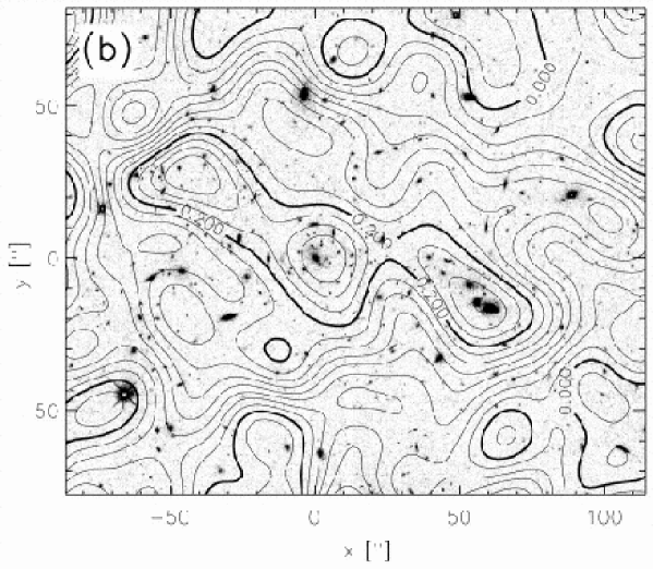
Figure 6: Mass reconstruction (contours) of the inner part of the high redshift ($z_{\rm d}=0.83$) cluster MS1054$-$03, based on a mosaic of six pointings obtained with the WFPC2@HST (from Hoekstra et al. 2000). The splitting of the cluster core into three subcomponents, previously seen from ground-based images by Clowe et al. (2000), shows that this cluster is not yet relaxed

The mass reconstruction techniques discussed above have been applied to quite a number of clusters up to now, yielding parameter-free mass maps. It is obvious that the quality of a mass map depends on the number density of galaxies that can be used for a shear estimate, which in turn depends on the depth and the seeing of the observational data. Furthermore, the mass profiles of clusters are much more reliably determined if the data field covers a large region, as boundary effects get minimized.

The first application of the Kaiser & Squires reconstruction technique was done to the X-ray detected cluster MS1224+20 (Fahlman et al. 1994); it resulted in an estimate of the mass-to-light ratio in this $z=0.33$ cluster of $\sim 800\,h$, considerably larger than ‘normal’ values of $M/L\sim 250\,h$. This conclusion was later reinforced by a fully independent weak-lensing analysis of this cluster by Fischer (1999). This mass estimate is in fact in conflict with the measured velocity dispersion of the cluster galaxies, which is much smaller than obtained by an SIS fit to the shear data. The line-of-sight to this cluster is fairly complicated, with additional peaks in the redshift distribution of galaxies in the field (Carlberg et al. 1994), all of which are included in the weak lensing measurement. Furthermore, this cluster may not be in a relaxed state, which probably renders the X-ray mass analysis inaccurate.

In fact, non-relaxed clusters are probably more common than naively expected. One example is shown in Fig. 6, a mass reconstruction of a high-redshift cluster based on HST data. The presence of three mass clumps, which coincide with three concentrations of cluster galaxies, indicates that this cluster is still in the process of merging. When the merging occurs along the line-of-sight, then it is less obvious in the mass maps. One example seems to be the cluster Cl0024+16, for which one obtains a large mass from the distance of its arcs from the cluster center (Colley et al. 1996), but which is fairly underluminous in X-rays for this mass. A detailed investigation of the structure of this cluster in radial velocity space by Czoske et al. (2002) has shown strong evidence for a collision of two clusters along the line-of-sight. Another example is provided by the cluster A1689, where the extended arc structures suggest an Einstein radius of about $40^{\prime\prime}$ for this cluster, making this the strongest lensing cluster in the sky, but the weak lensing results do not support the enormous mass obtained from the arcs (see Clowe & Schneider 2001, King et al. 2002, and references therein).

However, in many clusters the weak lensing mass estimates are in good agreement with those from dynamical estimates and X-ray determinations (e.g., Squires et al. 1996), provided the inner region of the clusters are omitted – but for them, the weak lensing method does not have sufficient angular resolution anyway. For example, Hoekstra and collaborators have observed three X-ray selected clusters with HST mosaics, and their results, summarized in Hoekstra et al. (2002a), shows that the SIS fit values for the velocity dispersion agree with those from spectrosopic investigations.

The mass maps can also be used to study how well the cluster galaxy distribution traces the underlying dark matter. An HST data based mass reconstruction of Cl0939+47 (Seitz et al. 1996) shows detailed structure that is very well matched with the distribution of bright cluster galaxies. A more quantitative investigation was performed by Wilson et al. (2001) showing that early-type galaxies trace the dark matter distribution quite well.

One of the predictions of CDM models for structure formation is that clusters of galaxies are located at the intersection points of filaments. In particular, this implies that a physical pair of clusters should be connected by a bridge or filament of (dark) matter, and weak lensing mass reconstructions can in principle be used to search for them. In the investigation of the $z=0.42$ supercluster MS0302, Kaiser et al. (1998) found an indication of a possible filament connecting two of the three clusters, with the caveat (as pointed out by the authors) that the filament lies just along the boundary of two CCD chips. Gray et al. (2002) saw a filament connecting the two clusters A901A/901B in their mass recosntruction of the A901/902 supercluster field. One of the problems related to the unambiguous detection of filaments is the difficulty to define what a ‘filament’ is, i.e. to device a statistics to quantify the presence of a mass bridge. Because of that, it is difficult to distinguish between noise in the mass maps, the ‘elliptical’ extension of two clusters pointing towards each other, and a true filament.

A perhaps surprising result is the difficulty of distinguishing between the NFW mass profile from, say power-law models, such as the isothermal profile. In fact, even from weak lensing observations covering large fields, out to the virial radius of clusters (Clowe & Schneider 2001, 2002; King et al. 2002), the distinction between NFW and isothermal is present only at the $\mathrel{\mathchoice{\lower 2.0pt\vbox{\halign{$\m@th\displaystyle\hfil#\hfil$\cr<\crcr\sim\crcr}}}{\lower 2.0pt\vbox{\halign{$\m@th\textstyle\hfil#\hfil$\cr<\crcr\sim\crcr}}}{\lower 2.0pt\vbox{\halign{$\m@th\scriptstyle\hfil#\hfil$\cr<\crcr\sim\crcr}}}{\lower 2.0pt\vbox{\halign{$\m@th\scriptscriptstyle\hfil#\hfil$\cr<\crcr\sim\crcr}}}}2\sigma$ level. The reason for this is the mass-sheet degeneracy. Within a family of models (such as the NFW), the model parameters can be determined with fairly high accuracy. One way to improve on the distinction between various mass profiles is to incorporate strong lensing constraints into the mass reconstruction (e.g., using inverse methods; see below). In particular, the multiple images seen in the cores of clusters can be used to determine the central mass profile (see Sand et al. 2002; Gavazzi et al. 2003). On the other hand, one can statistically superpose weak lensing measurements of clusters to obtain their average mass profile, as done by Dahle et al. (2003) for six clusters; even in that case, a (generalized) NFW profile is hardly distinguishable from an isothermal model.

5.4.4 Inverse methods

In addition to these ‘direct’ methods for determing $\kappa$, inverse methods have been developed, such as a maximum-likelihood fit (Bartelmann et al. 1996) to the data. In these techniques, one parameterizes the lens by the deflection potential $\psi$ on a grid and then maximizes

$${\cal L}=\prod_{i=1}^{N_{\rm g}}{1\over\pi\,\sigma_{i}^{2}\left({\hbox{$\bf\theta$}}_{i},\{\psi_{n}\}\right)}\exp\left(-\frac{|\epsilon_{i}-g\left({\hbox{$\bf\theta$}}_{i},\{\psi_{n}\}\right)|^{2}}{\sigma_{i}^{2}\left({\hbox{$\bf\theta$}}_{i},\{\psi_{n}\}\right)}\right)$$ (5.12)

with respect to these gridded $\psi$-values. In order to avoid overfitting, one needs a regularization; entropy regularization (Seitz et al. 1998) seems best suited. It should be pointed out that the deflection potential $\psi$, and not the surface mass density $\kappa$, should be used as a variable, for two reasons: first, shear and $\kappa$ depend locally on $\psi$, and are thus readily calculated by finite differencing, whereas the relation between $\gamma$ and $\kappa$ is non-local and requires summation over all gridpoints. Second, and more importantly, the surface mass density on a finite field does not determine $\gamma$ on this field, since mass outside the field contributes to $\gamma$ as well.

There are a number of reasons why inverse methods are in principle preferable to the direct method discussed above. First, in the direct methods, the smoothing scale is set arbitrarily, and in general kept constant. It would be useful to have an objective way how to choose this scale, and perhaps, the smoothing scale be a function of position: e.g., in regions with larger number densities of sources, the smoothing scale could be reduced. Second, the direct methods do not allow additional input coming from observations; for example, if both shear and magnification information are available, the latter could not be incorporated into the mass reconstruction. The same is true for clusters where strong lensing constraints are known.

5.5 Aperture mass

In the weak lensing regime, $\kappa\ll 1$, the mass-sheet degeneracy corresponds to adding a uniform surface mass density $\kappa_{0}$. We shall now consider a quantity, linearly related to $\kappa$, that is unaffected by the mass-sheet degeneracy. Let $U\left(|{\hbox{$\bf\theta$}}|\right)$ be a compensated weight (or filter) function, with $\int{\rm d}\theta\;\theta\,U(\theta)=0$, then the aperture mass

$$M_{\rm ap}({\hbox{$\bf\theta$}}_{0})=\int{\rm d}^{2}\theta\,\kappa({\hbox{$\bf\theta$}})\,U(|{\hbox{$\bf\theta$}}-{\hbox{$\bf\theta$}}_{0}|)$$ (5.13)

is independent of $\kappa_{0}$, as can be easily seen. The important point to notice is that $M_{\rm ap}$ can be written directly in terms of the shear (Schneider 1996)

$$\framebox{$\displaystyle M_{\rm ap}({\hbox{$\bf\theta$}}_{0})=\int{\rm d}^{2}\theta\,{Q(|{\hbox{$\bf\theta$}}|)}\,\gamma_{\rm t}({\hbox{$\bf\theta$}};{\hbox{$\bf\theta$}}_{0})$}\;,$$ (5.14)

where we have defined the tangential component $\gamma_{\rm t}$ of the shear relative to the point ${\hbox{$\bf\theta$}}_{0}$, and

$$Q(\theta)={2\over\theta^{2}}\int_{0}^{\theta}{\rm d}\theta^{\prime}\;\theta^{\prime}\,U(\theta^{\prime})-U(\theta)\;.$$ (5.15)

These relations can be derived from (5.7), by rewriting the partial derivatives in polar coordinates and subsequent integration by parts.

We shall now consider a few properties of the aperture mass.

• If $U$ has finite support, then $Q$ has finite support. This implies that the aperture mass can be calculated on a finite data field.

• If $U(\theta)={\rm const.}$ for $0\leq\theta\leq\theta_{\rm in}$, then $Q(\theta)=0$ for the same interval. Therefore, the strong lensing regime (where the shear $\gamma$ deviates significantly from the reduced shear $g$) can be avoided by properly choosing $U$ (and $Q$).

• If $U(\theta)=(\pi\theta_{\rm in}^{2})^{-1}$ for $0\leq\theta\leq\theta_{\rm in}$, $U(\theta)=-[\pi(\theta_{\rm out}^{2}-\theta_{\rm in}^{2})]^{-1}$ for $\theta_{\rm in}<\theta\leq\theta_{\rm out}$, and $U=0$ for $\theta>\theta_{\rm out}$, then $Q(\theta)=\theta_{\rm out}^{2}\,\theta^{-2}\left[\pi(\theta_{\rm out}^{2}-\vartheta_{\rm in}^{2})\right]^{-1}$ for $\theta_{\rm in}\leq\theta\leq\theta_{\rm out}$, and $Q(\theta)=0$ otherwise. For this special choice of $U$,

  $$M_{\rm ap}=\bar{\kappa}(\theta_{\rm in})-\bar{\kappa}(\theta_{\rm in},\theta_{\rm out})\;,$$ (5.16)

  the mean mass density inside $\theta_{\rm in}$ minus the mean density in the annulus $\theta_{\rm in}\leq\theta\leq\theta_{\rm out}$. Since the latter is non-negative, this yields lower limit to $\bar{\kappa}(\theta_{\rm in})$, and thus to $M(\theta_{\rm in})$.

6 Cosmic shear – lensing by the LSS

Up to now we have considered the lensing effect of localized mass concentrations, like galaxies and clusters. In addition to that, light bundles propagating through the Universe are continuously deflected and distorted by the gravitational field of the inhomogeneous mass distribution, the large-scale structure (LSS) of the cosmic matter field (the reader is referred to John Peacock’s lecture for the definition of cosmological parameters and the theory of structure growth in the Universe). This distortion of light bundles causes shape distortions of images of distant galaxies, and therefore, the statistics of the distortions reflect the statistical properties of the LSS.

Cosmic shear deals with the investigation of this connection, from the measurement of the correlated image distortion to the inference of cosmological information from this distortion statistics. As we shall see, cosmic shear has become a very important tool in observational cosmology. From a technical point-of-view, it is quite challenging, first because the distortions are indeed very weak and therefore difficult to measure, and second, in contrast to ‘ordinary’ lensing, here the light deflection does not occur in a ‘lens plane’ but by a 3-D matter distribution; one therefore needs a different description of the lensing optics. We start by looking at the description of light propagating through the Universe.

6.1 Light propagation in an inhomogeneous Universe

The laws of light propagation follow from Einstein’s General Relativity; according to it, light propagates along the null-geodesics of the space-time metric. As shown in SEF, one can derive from General Relativity that the governing equation for the propagation of thin light bundles through an arbitrary space-time is the equation of geodesic deviation,

$$\frac{{\rm d}^{2}{\hbox{$\bf\xi$}}}{{\rm d}\lambda^{2}}={\mathcal{T}}\,{\hbox{$\bf\xi$}}\;,$$ (6.1)

where $\bf\xi$ is the separation vector of two neighboring light rays, $\lambda$ the affine parameter along the central ray of the bundle, and ${\mathcal{T}}$ is the optical tidal matrix which describes the influence of space-time curvature on the propagation of light. ${\mathcal{T}}$ can be expressed directly in terms of the Riemann curvature tensor.

For the case of a weakly inhomogeneous Universe, the tidal matrix can be explicitly calculated in terms of the Newtonian potential. For that, we write the slightly perturbed metric of the Universe in the form

$${\rm d}s^{2}=a^{2}(\tau)\left[\left(1+\frac{2\Phi}{c^{2}}\right)\,c^{2}{\rm d}\tau^{2}-\left(1-\frac{2\Phi}{c^{2}}\right)\left({\rm d}w^{2}+f_{K}^{2}(w){\rm d}\omega^{2}\right)\right]\;,$$ (6.2)

where $w$ is the comoving radial distance, $a=(1+z)^{-1}$ the scale factor, normalized to unity today, $\tau$ is the conformal time, related to the cosmic time $t$ through ${\rm d}t=a\;{\rm d}\tau$, $f_{K}(w)$ is the comoving angular diameter distance, which equals $w$ in a spatially flat model, and $\Phi$ denotes the Newtonian peculiar gravitational potential. In this metric, the equation of geodesic deviation yields, for the comoving separation vector ${\hbox{$\bf x$}}({\hbox{$\bf\theta$}},w)$ between a ray separated by an angle $\bf\theta$ at the observer from a fiducial ray, the evolution equation

$$\frac{{\rm d}^{2}{\hbox{$\bf x$}}}{{\rm d}w^{2}}+K\,{\hbox{$\bf x$}}=-\frac{2}{c^{2}}\left[\nabla_{\perp}\Phi\left({\hbox{$\bf x$}}({\hbox{$\bf\theta$}},w),w\right)-\nabla_{\perp}\Phi^{(0)}\left(w\right)\right]\;,$$ (6.3)

where $K=(H_{0}/c)^{2}\,(\Omega_{\rm m}+\Omega_{\Lambda}-1)$ is the spatial curvature, $\nabla_{\perp}=(\partial/\partial x_{1},\partial/\partial x_{2})$ is the transverse comoving gradient operator, and $\Phi^{(0)}(w)$ is the potential along the fiducial ray. The formal solution of the transport equation is obtained by the method of Green’s function, to yield

$${\hbox{$\bf x$}}({\hbox{$\bf\theta$}},w)=f_{K}(w){\hbox{$\bf\theta$}}-\frac{2}{c^{2}}\int_{0}^{w}\!{\rm d}w^{\prime}\,f_{K}(w-w^{\prime})\left[\nabla_{\perp}\Phi\left({\hbox{$\bf x$}}({\hbox{$\bf\theta$}},w^{\prime}),w^{\prime}\right)-\nabla_{\perp}\Phi^{(0)}\left(w^{\prime}\right)\right]\;.$$ (6.4)

A source at comoving distance $w$ with comoving separation $\bf x$ from the fiducial light ray would be seen, in the absence of lensing, at the angular separation ${\hbox{$\bf\beta$}}={\hbox{$\bf x$}}/f_{K}(w)$ from the fiducial ray (this statement is nothing but the definition of the comoving angular diameter distance). Hence, in analogy with standard lens theory, we define the Jacobian matrix

$${\cal A}({\hbox{$\bf\theta$}},w)={\partial{\hbox{$\bf\beta$}}\over\partial{\hbox{$\bf\theta$}}}={1\over f_{K}(w)}{\partial{\hbox{$\bf x$}}\over\partial{\hbox{$\bf\theta$}}}\;,$$ (6.5)

and obtain

$${\cal A}_{ij}({\hbox{$\bf\theta$}},w)=\delta_{ij}-\frac{2}{c^{2}}\int_{0}^{w}\!\!{\rm d}w^{\prime}\,{f_{K}(w-w^{\prime})f_{K}(w^{\prime})\over f_{K}(w)}\,\Phi_{,ik}\left({\hbox{$\bf x$}}({\hbox{$\bf\theta$}},w^{\prime}),w^{\prime}\right)\,{\cal A}_{kj}({\hbox{$\bf\theta$}},w^{\prime})\;,$$ (6.6)

which describes the locally linearized mapping introduced by LSS lensing. This equation still is exact in the limit of validity of the weak-field metric. Next, we expand ${\cal A}$ in powers of $\Phi$, and truncate the series after the linear term:

$$\framebox{$\displaystyle{\cal A}_{ij}({\hbox{$\bf\theta$}},w)=\delta_{ij}-\frac{2}{c^{2}}\int_{0}^{w}\!\!{\rm d}w^{\prime}\,{f_{K}(w-w^{\prime})f_{K}(w^{\prime})\over f_{K}(w)}\,\Phi_{,ij}\left(f_{K}(w^{\prime}){\hbox{$\bf\theta$}},w^{\prime}\right)$}\;.$$ (6.7)

Hence, to linear order, the distortion can be obtained by integrating along the unperturbed ray; this is also called the Born approximation. Corrections to the Born approximation are necessarily of order $\Phi^{2}$. If we now define the deflection potential

$$\psi({\hbox{$\bf\theta$}},w):=\frac{2}{c^{2}}\int_{0}^{w}\!\!{\rm d}w^{\prime}\,{f_{K}(w-w^{\prime})f_{K}(w^{\prime})\over f_{K}(w)}\,\Phi\left(f_{K}(w^{\prime}){\hbox{$\bf\theta$}},w^{\prime}\right)$$ (6.8)

then ${\cal A}_{ij}=\delta_{ij}-\psi_{,ij}$, just as in ordinary lens theory. In this approximation, lensing by the 3-D matter distribution can be treated as an equivalent lens plane with deflection potential $\psi$, mass density $\kappa=\nabla^{2}\psi/2$, and shear $\gamma=(\psi_{,11}-\psi_{,22})/2+{\rm i}\psi_{,12}$.

6.2 Cosmic shear: the principle

6.2.1 The effective surface mass density

Next, we relate $\kappa$ to the fractional density contrast $\delta$ of matter fluctuations in the Universe; this is done in a number of steps:

1. Take the 2-D Laplacian of $\psi$, and add the term $\Phi_{,33}$ in the integrand; this latter term vanishes in the line-of-sight integration, as can be seen by integration by parts.

2. We make use of the 3-D Poisson equation in comoving coordinates

   $$\nabla^{2}\Phi={3H_{0}^{2}\Omega_{\rm m}\over 2a}\delta$$ (6.9)

   to obtain

   $$\framebox{$\displaystyle\kappa({\hbox{$\bf\theta$}},w)=\frac{3H_{0}^{2}\Omega_{\rm m}}{2c^{2}}\,\int_{0}^{w}\,{\rm d}w^{\prime}\,\frac{f_{K}(w^{\prime})f_{K}(w-w^{\prime})}{f_{K}(w)}\,\frac{\delta\left(f_{K}(w^{\prime}){\hbox{$\bf\theta$}},w^{\prime}\right)}{a(w^{\prime})}$}\;.$$ (6.10)

   Note that $\kappa$ is proportional to $\Omega_{\rm m}$, since lensing is sensitive to $\Delta\rho\propto\Omega_{\rm m}\,\delta$, not just to the density contrast $\delta=\Delta\rho/\bar{\rho}$ itself.

3. For a redshift distribution of sources with $p_{z}(z)\,{\rm d}z=p_{w}(w)\,{\rm d}w$, the effective surface mass density becomes

   $$\framebox{$\displaystyle\kappa({\hbox{$\bf\theta$}})=\int{\rm d}w\;p_{w}(w)\,\kappa({\hbox{$\bf\theta$}},w)=\frac{3H_{0}^{2}\Omega_{\rm m}}{2c^{2}}\,\int_{0}^{w_{\rm h}}{\rm d}w\;g(w)\,f_{K}(w)\,\frac{\delta\left(f_{K}(w){\hbox{$\bf\theta$}},w\right)}{a(w)}$}$$ (6.11)

   with

   $$\framebox{$\displaystyle g(w)=\int_{w}^{w_{\rm h}}{\rm d}w^{\prime}\;p_{w}(w^{\prime}){f_{K}(w^{\prime}-w)\over f_{K}(w^{\prime})}$}\;,$$ (6.12)

   which is essentially the source-redshift weighted lens efficiency factor $D_{\rm ds}/D_{\rm s}$ for a density fluctuation at distance $w$, and $w_{\rm h}$ is the comoving horizon distance.

6.2.2 Limber’s equation

The density field $\delta$ is assumed to be a realization of a random field. It is the properties of the random field that cosmologists can predict. In particular, the second-order statistical properties of the density field are described in terms of the power spectrum. We shall therefore look at the relation between the quantities relevant for lensing and the power spectrum. The basis of this relation is Limber’s equation. If $\delta$ is a homogeneous and isotropic 3-D random field, then the projections

$$g_{i}({\hbox{$\bf\theta$}})=\int{\rm d}w\;q_{i}(w)\,\delta\left(f_{K}(w){\hbox{$\bf\theta$}},w\right)$$ (6.13)

also are (2-D) homogeneous and isotropic random fields, where the $q_{i}$ are weight functions. In particular, the correlation function

$$C_{12}=\left\langle g_{1}({\hbox{$\bf\varphi$}}_{1})\,g_{2}({\hbox{$\bf\varphi$}}_{2})\right\rangle\equiv C_{12}(|{\hbox{$\bf\varphi$}}_{1}-{\hbox{$\bf\varphi$}}_{2}|)$$ (6.14)

depends only on the modulus of the separation vector. The original form of the Limber equation relates $C_{12}$ to the correlation function of $\delta$ which is a line-of-sight projection. Alternatively, one can consider the Fourier-space version of this relation: The power spectrum $P_{12}(\ell)$ – the Fourier transform of $C_{12}(\theta)$ – depends linearly on the power spectrum $P_{\delta}(k)$ of the density fluctuations (Kaiser 1992),

$$\framebox{$\displaystyle P_{12}(\ell)=\int{\rm d}w\;{q_{1}(w)\,q_{2}(w)\over f_{K}^{2}(w)}\,P_{\delta}\left({\ell\over f_{K}(w)},w\right)$}\;,$$ (6.15)

if the largest-scale structures in $\delta$ are much smaller than the effective range $\Delta w$ of the projection. Hence, we obtain the (very reasonable) result that the power at angular scale $1/\ell$ is obtained from the 3-D power at length scale $f_{K}(w)\,(1/\ell)$, integrated over $w$. Comparing (5.8) with (6.15), one sees that $\kappa({\hbox{$\bf\theta$}})$ is such a projection of $\delta$ with the weights $q_{1}(w)=q_{2}(w)=(3/2)(H_{0}/c)^{2}\Omega_{\rm m}g(w)f_{K}(w)/a(w)$, so that

$$\framebox{$\displaystyle P_{\kappa}(\ell)=\frac{9H_{0}^{4}\Omega_{\rm m}^{2}}{4c^{4}}\,\int_{0}^{w_{\rm h}}{\rm d}w\,\frac{g^{2}(w)}{a^{2}(w)}\,P_{\delta}\left(\frac{\ell}{f_{K}(w)},w\right)$}\;.$$ (6.16)

The power spectrum $P_{\kappa}$, if obtained through observations, can therefore be used to constrain the 3-D power spectrum $P_{\delta}$.

6.3 Second-order cosmic shear measures

As we shall see, all second-order statistics of the cosmic shear yield (filtered) information about $P_{\kappa}$. The most-often used second-order statistics are:

• The two-point correlation function(s) of the shear, $\xi_{\pm}(\theta)$,

• the shear dispersion in a (circular) aperture, $\left\langle|\bar{\gamma}|^{2}\right\rangle(\theta)$, and

• the aperture mass dispersion, $\left\langle M_{\rm ap}^{2}\right\rangle(\theta)$.

These will be discussed next, and their relation to $P_{\kappa}(\ell)$ shown. As a preparation, consider the Fourier transform of $\kappa$,

$$\hat{\kappa}({\hbox{$\bf\ell$}})=\int{\rm d}^{2}\theta\,{\rm e}^{{\rm i}{\hbox{$\bf\ell$}}\cdot{\hbox{$\bf\theta$}}}\,\kappa({\hbox{$\bf\theta$}})\;;$$ (6.17)

then,

$$\left\langle\hat{\kappa}({\hbox{$\bf\ell$}})\hat{\kappa}^{*}({\hbox{$\bf\ell$}}^{\prime})\right\rangle=(2\pi)^{2}\,\delta_{\rm D}({\hbox{$\bf\ell$}}-{\hbox{$\bf\ell$}}^{\prime})\,P_{\kappa}(\ell)\;,$$ (6.18)

which provides another definition of the power spectrum $P_{\kappa}$. The Fourier transform of the shear is

$$\hat{\gamma}({\hbox{$\bf\ell$}})=\left(\ell_{1}^{2}-\ell_{2}^{2}+2{\rm i}\ell_{1}\ell_{2}\over\left|{\hbox{$\bf\ell$}}\right|^{2}\right)\hat{\kappa}({\hbox{$\bf\ell$}})$$ (6.19)

which implies that

$$\left\langle\hat{\gamma}({\hbox{$\bf\ell$}})\hat{\gamma}^{*}({\hbox{$\bf\ell$}}^{\prime})\right\rangle=(2\pi)^{2}\,\delta_{\rm D}({\hbox{$\bf\ell$}}-{\hbox{$\bf\ell$}}^{\prime})\,P_{\kappa}(\ell).$$ (6.20)

Hence, the power spectrum of the shear is the same as that of the convergence.

6.3.1 Shear correlation functions

Consider a pair of points (i.e., galaxy images); their separation direction $\varphi$ (i.e. the polar angle of the separation vector $\bf\theta$) is used to define the tangential and cross-component of the shear at these positions for this pair,

$$\gamma_{\rm t}=-{\cal R}\hbox{e}\left(\gamma\,{\rm e}^{-2{\rm i}\varphi}\right)\;,\quad\gamma_{\times}=-{\cal I}\hbox{m}\left(\gamma\,{\rm e}^{-2{\rm i}\varphi}\right)\;.$$ (6.21)

Then, the shear correlation functions are defined as

$$\xi_{\pm}(\theta) = \left\langle\gamma_{\rm t}\gamma_{\rm t}\right\rangle\pm\left\langle\gamma_{\times}\gamma_{\times}\right\rangle(\theta)\;,$$

$$\xi_{\times}(\theta) = \left\langle\gamma_{\rm t}\gamma_{\times}\right\rangle(\theta)\;.$$

Due to parity symmetry, $\xi_{\times}(\theta)$ is expected to vanish, since under such a transformation, $\gamma_{\rm t}\to\gamma_{\rm t}$, but $\gamma_{\times}\to-\gamma_{\times}$. Next we relate the shear correlation functions to the power spectrum $P_{\kappa}$: Using the definition of $\xi_{\pm}$, replacing $\gamma$ in terms of $\hat{\gamma}$, and making use of relation between $\hat{\gamma}$ and $\hat{\kappa}$, one finds:

$$\framebox{$\displaystyle\xi_{+}(\theta)=\int_{0}^{\infty}{{\rm d}\ell\,\ell\over 2\pi}\,{\rm J}_{0}(\ell\theta)\,P_{\kappa}(\ell)\;;\;\;\xi_{-}(\theta)=\int_{0}^{\infty}{{\rm d}\ell\,\ell\over 2\pi}\,{\rm J}_{4}(\ell\theta)\,P_{\kappa}(\ell)$}\;.$$ (6.22)

$\xi_{\pm}$ can be measured as follows: on a data field, select all pairs of faint galaxies with separation within $\Delta\theta$ of $\theta$ and then take the average $\left\langle{\epsilon}_{{\rm t}i}\,{\epsilon}_{{\rm t}j}\right\rangle$ over all these pairs; since ${\epsilon}={\epsilon}^{(\rm s)}+\gamma({\hbox{$\bf\theta$}})$, the expectation value of $\left\langle{\epsilon}_{{\rm t}i}\,{\epsilon}_{{\rm t}j}\right\rangle$ is $\left\langle\gamma_{\rm t}\gamma_{\rm t}\right\rangle(\theta)$, provided source ellipticities are uncorrelated. Similarly, the correlation for the cross-components is obtained.

6.3.2 The shear dispersion

Consider a circular aperture of radius $\theta$; the mean shear in this aperture is $\bar{\gamma}$. Averaging over many such apertures, one defines the shear dispersion $\left\langle|\bar{\gamma}|^{2}\right\rangle(\theta)$. It is related to the power spectrum through

$$\framebox{$\displaystyle\left\langle\left|\bar{\gamma}\right|^{2}\right\rangle(\theta)={1\over 2\pi}\int{\rm d}\ell\,\ell\,P_{\kappa}(\ell)\,W_{\rm TH}(\ell\theta)$}\;,\;\;{\rm where}\;\;W_{\rm TH}(\eta)={4{\rm J}_{1}^{2}(\eta)\over\eta^{2}}$$ (6.23)

is the top-hat filter function. The shear dispersion can be measured by averaging the square of the mean galaxy ellipticities over many independent apertures.

6.3.3 The aperture mass

Consider a circular aperture of radius $\theta$; for a point inside the aperture, define the tangential and cross-components of the shear relative to center of aperture (as before); then define

$$M_{\rm ap}(\theta)=\int{\rm d}^{2}{\vartheta}\;Q(|{\hbox{$\bf{\vartheta}$}}|)\,\gamma_{\rm t}({\hbox{$\bf{\vartheta}$}})\;,$$ (6.24)

where $Q$ is a weight function with support ${\vartheta}\in[0,\theta]$. In the following we shall use

$$Q({\vartheta})={6\over\pi\theta^{2}}\,{{\vartheta}^{2}\over\theta^{2}}\left(1-{{\vartheta}^{2}\over\theta^{2}}\right)\,{\rm H}(\theta-{\vartheta})\;,$$

in which case the dispersion of $M_{\rm ap}(\theta)$ is related to the power spectrum by

$$\framebox{$\displaystyle\left\langle M_{\rm ap}^{2}\right\rangle(\theta)={1\over 2\pi}\int_{0}^{\infty}{\rm d}\ell\;\ell\,P_{\kappa}(\ell)\,W_{\rm ap}(\theta\ell)$}\;,\;\;{\rm with}\;\;W_{\rm ap}(\eta):={576{\rm J}_{4}^{2}(\eta)\over\eta^{4}}\;.$$ (6.25)

6.3.4 Interrelations

These various 2-point statistics all depend linearly on the power spectrum $P_{\kappa}$; therefore, one should not be too surprised that they are all related to each other. The surprise perhaps is that these interrelations are quite simple (Crittenden et al. 2002). First, the relations between $\xi_{\pm}$ and $P_{\kappa}$ can be inverted, making use of the orthonormality relation of Bessel functions:

$$P_{\kappa}(\ell)=2\pi\int_{0}^{\infty}{\rm d}\theta\,\theta\,\xi_{+}(\theta)\,{\rm J}_{0}(\ell\theta)=2\pi\int_{0}^{\infty}{\rm d}\theta\,\theta\,\xi_{-}(\theta)\,{\rm J}_{4}(\ell\theta)\;.$$ (6.26)

Next, we take one of these and plug it into the relation between the other correlation function and $P_{\kappa}$, to find:

$$\framebox{$\displaystyle\xi_{+}(\theta)=\xi_{-}(\theta)+\int_{\theta}^{\infty}{{\rm d}{\vartheta}\over{\vartheta}}\xi_{-}({\vartheta})\left(4-12{\theta^{2}\over{\vartheta}^{2}}\right)$}\;;$$ (6.27)

$$\framebox{$\displaystyle\xi_{-}(\theta)=\xi_{+}(\theta)+\int_{0}^{\theta}{{\rm d}{\vartheta}\,{\vartheta}\over\theta^{2}}\xi_{+}({\vartheta})\left(4-12{{\vartheta}^{2}\over\theta^{2}}\right)$}\,.$$ (6.28)

Using (6.26) in the expression for the shear dispersion, one finds

$$\framebox{$\displaystyle\left\langle\left|\bar{\gamma}\right|^{2}\right\rangle(\theta)=\int_{0}^{2\theta}{{\rm d}{\vartheta}\,{\vartheta}\over\theta^{2}}\;\xi_{+}({\vartheta})\,S_{+}\left({\vartheta}\over\theta\right)=\int_{0}^{\infty}{{\rm d}{\vartheta}\,{\vartheta}\over\theta^{2}}\;\xi_{-}({\vartheta})\,S_{-}\left({\vartheta}\over\theta\right)$}\;,$$ (6.29)

where the $S_{\pm}$ are simple functions, given explicitly in Schneider et al. (2002a). Finally, the same procedure for the aperture mass dispersion lets us write

$$\framebox{$\displaystyle\left\langle M_{\rm ap}^{2}\right\rangle(\theta)=\int_{0}^{2\theta}{{\rm d}{\vartheta}\,{\vartheta}\over\theta^{2}}\;\xi_{+}({\vartheta})\,T_{+}\left({\vartheta}\over\theta\right)=\int_{0}^{2\theta}{{\rm d}{\vartheta}\,{\vartheta}\over\theta^{2}}\;\xi_{-}({\vartheta})\,T_{-}\left({\vartheta}\over\theta\right)$}\;,$$ (6.30)

again with known functions $T_{\pm}$ (Schneider et al. 2002a). Hence, all these 2-point statistics can be evaluated from the correlation functions $\xi_{\pm}(\theta)$, which is of particular interest, since they can be measured best: Real data fields contain holes and gaps (like CCD defects, brights stars, nearby galaxies, etc.) which makes the placing of apertures difficult; however, the evaluation of the correlation functions is not affected by gaps, as one uses all pairs of galaxy images with a given angular separation.

6.4 Cosmic shear and cosmology

6.4.1 Why cosmology from cosmic shear?

Before continuing, it is worth to pause for a second and ask the question as to why one tries to investigate cosmological questions by using cosmic shear – since the CMB can measure cosmological parameters with high accuracy. Partial answers to this question are:

• Cosmic shear measures the mass distribution at much lower redshifts ($z\mathrel{\mathchoice{\lower 2.0pt\vbox{\halign{$\m@th\displaystyle\hfil#\hfil$\cr<\crcr\sim\crcr}}}{\lower 2.0pt\vbox{\halign{$\m@th\textstyle\hfil#\hfil$\cr<\crcr\sim\crcr}}}{\lower 2.0pt\vbox{\halign{$\m@th\scriptstyle\hfil#\hfil$\cr<\crcr\sim\crcr}}}{\lower 2.0pt\vbox{\halign{$\m@th\scriptscriptstyle\hfil#\hfil$\cr<\crcr\sim\crcr}}}}1$) and at smaller physical scales [$R\sim 0.3\,h^{-1}\,(\theta/1^{\prime})\,{\rm Mpc}$] than the CMB; indeed, it is the only way to map out the dark matter distribution directly without any assumptions about the relation between dark and baryonic matter. The smaller scales probed are very important for constraining the shape of the power spectrum, i.e., the primordial tilt and the shape parameter $\Gamma_{\rm spect}$.

• Cosmic shear measures the non-linearly evolved mass distribution and its associated power spectrum $P_{\delta}(k)$; hence, in combination with the CMB it allows us to study the evolution of the power spectrum and in particular, provides a very powerful test of the gravitational instability paradigm for structure growth.

• It provides a fully independent way to probe the cosmological model. Given the revolutionary claims coming from the CMB, SN Ia, and the LSS of the galaxy distribution, namely that more than 95% of the stuff in the Universe is in a form about whose physical nature we have not the slightest idea, an additional independent verification of these claims is certainly welcome.

• As we shall see shortly, cosmic shear studies provide a new and highly valuable search method for cluster-scale matter concentrations.

6.4.2 Expectations

The cosmic shear signal depends on the cosmological model, parametrized by $\Omega_{\rm m}$, $\Omega_{\Lambda}$, and the shape parameter $\Gamma_{\rm spect}$ of the power spectrum, the normalization of the power spectrum, usually expressed in terms of $\sigma_{8}$, and the redshift distribution of the sources. By measuring $\xi_{\pm}$ over a significant range of angular scales one can derive constraints on these parameters.

The accuracy with which $\xi_{\pm}$ can be measured depends on number density of galaxies (that is, depth and quality of the images), the total solid angle covered by the survey, and its geometric arrangement (compact survey vs. widely separated pointings); it is determined by a combination of intrinsic ellipticity dispersion and the cosmic (or sampling) variance. For angular scales below about 1 degree, the non-linear evolution of the power spectrum becomes important for the cosmic shear signal; because of this, the expected signal is considerably larger than estimated from linear perturbation theory of structure evolution. Furthermore, the signal depends quite strongly on the mean redshift of the source galaxies, which suggests that deep surveys, aiming for higher-redshift galaxies, are best suited for cosmic shear studies.

6.5 Observation of cosmic shear

6.5.1 First detections

Whereas the theory of cosmic shear was worked out in the early 1990’s (Blandford et al. 1991; Miralda-Escudé 1991; Kaiser 1992), it took until the year 2000 before this effect was first discovered. The reason for this time lag must be seen as a combination of instrumental developments, i.e. the wide-field CCD mosaic cameras, and the image analysis software, like IMCAT, with which shapes of galaxies can be corrected for PSF effects. Finally, in March 2000, four groups independently published their first discoveries of cosmic shear (Bacon et al. 2000; Kaiser et al. 2000; van Waerbeke et al. 2000, Wittman et al. 2000). In these surveys, of the order of $10^{5}$ galaxy images have been analyzed, covering about 1 deg². The fact that the results from these four independent teams agreed within the respective error bars immediately gave credence to this new window of observational cosmology. Furthermore, 4 different telescopes, 5 different cameras, independent data reduction tools and at least two different image analysis methods have been used in these studies. Maoli et al. (2001) reported a significant cosmic shear measurement from 50 widely separated FORS1@VLT images, which also agreed with the earlier measurements.

6.5.2 Deriving constraints

From the measured correlation functions $\xi_{\pm}(\theta)$, obtaining constraints on cosmological parameters can proceed through minimizing

$$\chi^{2}(p)=\sum_{ij}\left(\xi_{i}(p)-\xi_{i}^{\rm obs}\right)\,{\rm Cov}^{-1}_{ij}\,\left(\xi_{j}(p)-\xi_{j}^{\rm obs}\right)\;,$$ (6.31)

with $\xi_{i}=\xi(\theta_{i})$ being the binned correlation function(s) (i.e., either $\xi_{\pm}$, or using both), $p$ is a set of cosmological parameters, and ${\rm Cov}^{-1}_{ij}$ the inverse covariance matrix. The latter can be determined either from the $\xi_{\pm}$ itself, from simulations, or estimated from the data (see Schneider et al. 2002b). Nevertheless, the calculation of the covariance is fairly cumbersome, and most authors have used approximate methods to derive it, such as the field-to-field variations of the measured correlation. As it turns out, $\xi_{+}(\theta)$ is strongly correlated across angular bins, much less so for $\xi_{-}(\theta)$; this is due to the fact that the filter function that describes $\xi$ in terms of the power spectrum $P_{\kappa}$ is much broader for $\xi_{+}$ (namely ${\rm J}_{0}$) than ${\rm J}_{4}$ which applies for $\xi_{-}$. Of course, a corresponding figure-of-merit function can be defined for the other second-order shear statistics, with their respective covariance matrices, but as argued before, the correlation functions should be regarded as the basic observable statistics.

6.5.3 Recent results

Since the first detections of cosmic shear, described above, there have been a large number of measurements over the past three years. Instead of mentioning them all here, we refer the reader to the recent reviews by van Waerbeke & Mellier (2003) and Refregier (2003). State-of-the-art are deep surveys, similar to those with which the first cosmic shear results have been derived, but with significantly larger solid angle (van Waerbeke et al. 2001, 2002), or shallower surveys of much larger area (e.g., Hoekstra et al. 2002c; Jarvis et al. 2003). The results of these surveys, which contain of the order of $\sim 10^{6}$ galaxies, i.e., an order-of-magnitude more than the discovery surveys mentioned above, can be summarized roughly as follows:

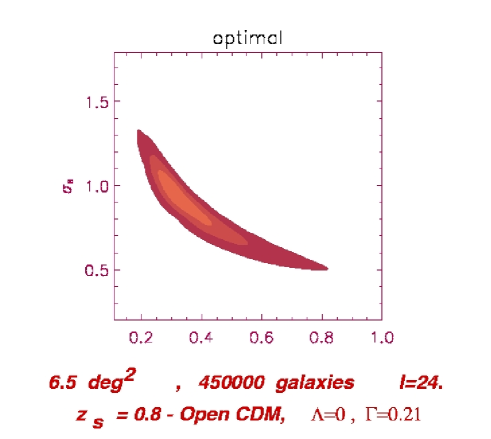
Figure 7: Constraints in the $\Omega_{\rm m}$ – $\sigma_{8}$ parameter plane, from the VIRMOS-DESCART survey (van Waerbeke et al. 2001). For this figure, in which the 1, 2, and 3-$\sigma$ confidence regions are indicated, a zero cosmological constant has been assumed, the redshift distribution of the source galaxies was assumed to be known, as well as the shape parameter $\Gamma_{\rm spect}=0.21$

Cosmic shear by itself presently does not provide strong constraints on multi-dimensional cosmological parameter space. Hence, if one does not fix most of the cosmological parameters from external sources, the allowed region in multi-dimensional parameter space is still quite large. On the other hand, if one considers a restricted set of parameters, cosmic shear results are very powerful. An example of that is given in Fig. 7, where all cosmological parameters have been kept fixed, except $\Omega_{\rm m}$ and the normalization $\sigma_{8}$. In this case, one finds indeed a well-defined maximum of the corresponding likelihood. Interestingly, the direction of the ‘likelihood valley’ nearly coincides with the constraint obtained from the cluster abundance, i.e., it provides a constraint on $\sigma_{8}\Omega_{\rm m}^{0.6}$. If the other cosmological parameters are not assumed to be known precisely, but are marginalized over a plausible uncertainty range, the likelihood contours widen substantially.

When combined with results from other methods, cosmic shear yields very useful information. For example, as pointed out by Hu & Tegmark (1999), when combined with data from CMB anisotropy, cosmic shear can break degeneracies of model parameters which are present when using the CMB data alone. In the $\Omega_{\rm m}$ – $\sigma_{8}$ parameter plane, cosmic shear constraints are nearly perpendicular to those from the CMB (van Waerbeke et al. 2002).

Therefore, at present the best use of cosmic shear results is in constraining the normalization $\sigma_{8}$ of the density perturbations, for a set of other cosmological parameters fixed by other methods, such as the CMB, galaxy redshift surveys, etc. The various cosmic shear surveys have given a range of $\sigma_{8}$ determinations which is about as narrow as current estimates from the abundance of massive clusters (see van Waerbeke & Mellier 2003 for a summary of these results). Given the youth of this field, this indeed is a remarkable achievement already. Furthermore, since the determination of $\sigma_{8}$ from cluster abundance and cosmic shear agree, one learns something important: the cluster abundance depends on the assumed Gaussianity of the primordial density field, whereas the constraint from cosmic shear does not. Hence, the agreement between the two methods supports the idea of an initial Gaussian field. Without doubt, the next generation of cosmic shear surveys will provide highly accurate determinations of this normalization, as well as other (combinations of) cosmological parameters.

6.6 E-modes, B-modes

In the derivation of the lensing properties of the LSS, we ended up with an equivalent surface mass density. In particular, this implied that ${\cal A}$ is a symmetric matrix, that the shear can be obtained in terms of $\kappa$ or $\psi$. Now, the shear is a 2-component quantity, whereas both $\kappa$ and $\psi$ are scalar fields. This implies that the two shear components are not independent of each other!

Recall that (5.7) yields a relation between the gradient of $\kappa$ and the first derivatives of the shear components; in particular, (5.7) implies that $\nabla\times{\hbox{$\bf u$}}_{\gamma}\equiv 0$, yielding a local constraint relation between the shear components. The validity of this constraint equation guarantees that the imaginary part of (5.4) vanishes. This constraint is also present at the level of 2-point statistics, since one expects from (6.26) that

$$\int_{0}^{\infty}{\rm d}\theta\,\theta\,\xi_{+}(\theta){\rm J}_{0}(\theta\ell)=\int_{0}^{\infty}{\rm d}\theta\,\theta\,\xi_{-}(\theta){\rm J}_{4}(\theta\ell)\;.$$ (6.32)

Hence, the two correlation functions $\xi_{\pm}$ are not independent. The observed shear field is not guaranteed to satisfy these relations, due to noise, remaining systematics, or other effects. Therefore, searching for deviations from this relation allows a check for these effects. However, there might also be a ‘shear’ component present that is not due to lensing (by a single equivalent thin matter sheet $\kappa$). Shear components which satisfy the foregoing relations are called E-modes; those which don’t are B-modes – these names are exported from the polarization of the CMB, which has the same mathematical properties as the shear field.

The best way to separate these modes locally is provided by the aperture measures: $\left\langle M^{2}_{\rm ap}(\theta)\right\rangle$ is sensitive only to E-modes. If one defines in analogy

$$M_{\perp}(\theta)=\int{\rm d}^{2}{\vartheta}\;Q(|{\hbox{$\bf{\vartheta}$}}|)\,\gamma_{\times}({\hbox{$\bf{\vartheta}$}})\;,$$ (6.33)

then $\left\langle M^{2}_{\perp}(\theta)\right\rangle$ is sensitive only to B-modes.

Figure 8: Dispersion of the aperture mass $\left\langle M_{\rm ap}^{2}\right\rangle$ (upper row) and its analogue $\left\langle M_{\perp}^{2}\right\rangle$ for the cross-component, as obtained from the Red Cluster Sequence survey (Hoekstra et al. 2002). The left panels show the results for a broad range of galaxy brightnesses, whereas the middle and right rows display the results for the bright and the fainter parts, respectively, of the sample. Clearly, the presence of the B-mode is seen; its strength decreases for the fainter part of the sample; this behavior is expected if the B-mode is due to intrinsic alignments of galaxies. Its relative importance decreases with increasing width of the redshift distribution of galaxies

Significant B-modes have been discovered in cosmic shear surveys (e.g., van Waerbeke et al. 2002; Hoekstra et al. 2002 – see Fig. 8); the question now is what are they due to? As mentioned before, the noise, which contributes to both E- and B-modes in similar strengths, could be underestimated, there could be remaining systematic effects, or indeed show the real presence of a B-mode on the sky. There are two possibilities known to generate a B-mode through lensing: The first-order in $\Phi$ (or ‘Born’) approximation may not be strictly valid, but as shown by ray-tracing simulations through cosmic matter fields (e.g., Jain et al. 2000) the resulting B-modes are expected to be very small. Clustering of sources also yields a finite B-mode (Schneider et al. 2002a), but again, this effect is much smaller than the observed amplitude of the B-modes.

Currently the best guess for the generation of a finite B-mode are intrinsic correlations of galaxy ellipticities. Such intrinsic alignments of galaxy ellipticities can be caused by the tidal gravitational field of the large-scale structure at galaxy formation. Predictions of the alignment of the projected ellipticity of the galaxy mass can be made analytically (e.g. tidal torque theory) or from numerical simulations; however, the predictions from various groups differ by large factors (e.g., Croft & Metzler 2000; Crittenden et al. 2001; Heavens et al. 2000; Jing 2002) which means that the process is not well understood at present. In addition, there remains the question of whether the orientation of the galaxy light (which is the issue of relevance here) is the same as that of the mass.

If intrinsic alignments play a role, then

$$\xi_{+}=\left\langle{\epsilon}_{i}\,{\epsilon}^{*}_{j}\right\rangle=\left\langle{\epsilon}_{i}^{(\rm s)}\,{\epsilon}^{(\rm s)*}_{j}\right\rangle+\xi_{+}^{\rm lens}\;,$$ (6.34)

and measured correlations $\xi_{\pm}$ contain both components. Of course, there is no reason why intrinsic correlations should have only an B-mode. If a B-mode contribution is generated through this process, then the measured E-mode is also contaminated by intrinsic alignments. In fact, the various models do not agree on the relative strength of E- and B-modes in the intrinsic alignments of galaxies, but it seems that the E-modes have generally higher amplitude than the B-modes. Given that intrinsic alignments yield ellipticity correlations only for spatially close sources (i.e., close in 3-D, not merely in projection), it is clear that the deeper a cosmic shear survey is, and thus the broader the redshift distribution, the smaller is the relative amplitude of an intrinsic signal. Most of the theoretical predictions on the strength of intrinsic alignments say that the deep cosmic shear surveys (say, with mean source redshifts of $\left\langle z_{\rm s}\right\rangle\sim 1$) are affected at a $\sim 10\%$ level, but that shallow cosmic shear surveys are more strongly affected; for them, the intrinsic alignment can be of the same order as, or larger than the lensing signal.

However, the intrinsic signal can be separated from the lensing signal if redshift information of the sources is available, owing to the fact that $\left\langle{\epsilon}_{i}^{(\rm s)}\,{\epsilon}^{(\rm s)*}_{j}\right\rangle$ will be non-zero only if the two galaxies are at the same redshift. Hence, if $z$-information is available (e.g., photometric redshifts), then galaxy pairs which are likely to have similar redshifts are to be avoided in estimating the cosmic shear signal (King & Schneider 2002; Heymans & Heavens 2003). This will change the expectation value of the shear correlation function, but in a controlable way, as the redshifts are assumed to be known. Indeed, using (photometric) redshifts, one can simultaneously determine the intrinsic and the lensing signal, essentially providing a cosmic shear tomography (King & Schneider 2003).

6.7 Higher-order statistics

On the level of second-order statistics, ‘only’ the power spectrum is probed. If the density field was Gaussian, then the power spectrum would fully characterize it; however, in the course of non-linear structure evolution, non-Gaussian features of the density field are generated, which show up correspondingly in the cosmic shear field and which can be probed by higher-order shear statistics. The usefulness of these higher-order measures for cosmic shear has been pointed out in Bernardeau et al. (1997) and van Waerbeke et al. (1999); in particular, the near-degeneracy between $\sigma_{8}$ and $\Omega_{\rm m}$ can be broken. However, these are serious problems with higher-order shear statistics, that shall be illustrated in terms of the third-order statistics. The three-point correlation function has three independent variables (e.g. the sides of a triangle) and 8 components; as was shown in Schneider & Lombardi (2003), none of these eight components vanishes owing to parity invariance. This then implies that the covariance matrix has 6 arguments and 64 components! Of course, this is too difficult to handle efficiently, and therefore one must ask which combinations of the components of the 3-pt correlation function are most useful for studying the dark matter distribution. Unfortunately, this is essentially unknown yet. An additional problem is that the predictions from theory are less well established than for the second-order statistics.

Nevertheless, progress has been made. From ray-tracing simulations through a cosmic matter distribution, the 3-pt correlation function of the shear can be determined (Takada & Jain 2003; see also Zaldarriaga & Scoccimarro 2003); in addition, Schneider & Lombardi (2003) have defined the ‘natural components’ of the 3-pt correlator which are most easily related to the bispectrum of the underlying matter distribution.

Alternatively, aperture measures can be defined to measure the third-order statistics. Schneider et al. (1998) calculated $\left\langle M_{\rm ap}^{3}\right\rangle(\theta)$ in the frame of the quasi-linear structure evolution model and showed it to be a strong function of $\Omega_{\rm m}$. Indeed, $\left\langle M_{\rm ap}^{3}\right\rangle$ is sensitive only to the E-modes of the shear field. One might be tempted to use $\left\langle M_{\perp}^{3}\right\rangle(\theta)$ as a measure for third-order B-mode statistics, but indeed, this quantity vanishes owing to parity invariance. However, $\left\langle M_{\perp}^{2}\,M_{\rm ap}\right\rangle$ is a measure for the B-modes at the third-order statistical level. Bernardeau et al. (2002) measured for the first time a significant 3-rd order shear from the VIRMOS-DESCART survey, employing a suitably filtered integral over the measured 3-pt correlation function. With the upcoming large cosmic shear surveys, the 3-pt function will be measured with high accuracy.

6.8 Weak lensing search for cluster-mass dark halos

As we have seen, the mass distribution of clusters of galaxies can be mapped by weak lensing techniques. In fact, the coherent alignment of background galaxy images clearly shows the presence of a massive matter concentration present at or near the location of the optically or X-ray selected cluster towards which the weak lensing observations were targeted. As pointed out in Schneider (1996), one can use weak lensing to search for clusters: seeing a strong alignment of galaxy images centered onto a point on a wide-field image, one would conclude the presence of the mass concentration there. A very useful way to quantify this is the aperture mass statistics, already introduced. By selecting an appropriate filter function, one can systematically seach for statistically significant peaks of $M_{\rm ap}$ on wide-field images. In fact, the data needed for this investigation is the same as that used in cosmic shear surveys.

Since clusters of galaxies are very important cosmological probes, e.g., to determine the normalization of the power spectrum of the matter inhomogeneities in the Universe, a selection of clusters based on their mass properties only would be extremely useful. Usually, clusters are selected by their optical or X-ray properties; to transform luminosity or X-ray temperature into a mass estimate, and thus to transform a flux-limited cluster sample into a mass-limited sample, which can then be compared to cosmological predictions, one needs to employ a number of approximations and scaling relations. In contrast to this, the shear selection can directly be compared to cosmological predictions, e.g., by calculating the abundance of peaks of $M_{\rm ap}$ directly from N-body simulations of structure formation (e.g., Reblinsky et al. 1999), without reliance on the luminous properties of baryonic matter, nor even for identifying cluster-mass halos in the simulated density fields.

The abundance of peaks above a given threshold $M_{\rm ap}$, at a given angular scale, can also be used as a cosmic shear measure. In fact, in future large cosmic shear surveys this will become most likely one of the most useful statistics for studying non-Gaussian aspects of the shear field. Within the frame of Press–Schechter theory, Kruse & Schneider (1999) calculated the $M_{\rm ap}$ peak statistics, which was then compared with direct numerical simulation by Reblinsky et al. (1999). White et al. (2002) pointed out that the $M_{\rm ap}$ statistics can be substantially affected by the large-scale structure along the line-of-sight to these mass concentrations; this implies that the relation between $M_{\rm ap}$ and the mass of the clusters is not simple – but again, this method does not require a mass function to be determined, as the $M_{\rm ap}$-statistics can be obtained directly from LSS simulations.

Several clusters, or cluster candidates, have been found that way. Erben et al. (2000) detected a highly significant shear signal corresponding to a putative mass peak, about $7^{\prime}$ away from the cluster Abell 1942, seen on two images taken with different filters and different cameras. No obvious concentration of galaxies is seen in this direction, neither in the optical nor near-IR images (Gray et al. 2001), making it a candidate for a ‘dark clump’; however, before drawing this conclusion, further investigations are needed, such as imaging with the HST to confirm the shear measurements. Umetsu & Futamase (2000) found a significant mass concentration on an HST image, again without an obvious optical counterpart. In contrast to this, Mellier et al. (2000) found a mass peak in one of their 50 VLT fields taken for a cosmic shear survey with FORS, which is clearly associated with a concentration of galaxies. Wittman et al. (2001, 2002) detected two clusters on their wide-field images, and confirmed them spectroscopically. In fact, making use of photometric redshift estimates of the background galaxies, and employing the redshift dependence of the lens strength, they were able to estimate rather precisely the cluster redshifts, which were later confirmed with spectroscopy. Two of the three putative mass concentrations found by Dahle et al. (2002) are also very likely to be associated with luminous clusters. Hence, the shear selection of clusters has already been proven as a very useful concept.

6.9 Lensing in three dimensions

Using (photometric) redshift estimates in cosmic shear research is not only useful to remove the potential contribution from intrinsic alignments of galaxy ellipticities. If one defines galaxy populations with different redshift distributions, one can probe different projections of the cosmic density field; see (5.8). This then increases the information one can extract from a cosmic shear survey, and thus the ability to discriminate between different cosmological models (Hu 1999).

More recently, it was pointed out (Taylor 2001; Hu & Keeton 2002) that the use of redshift information can in principle be used to reconstruct the three-dimensional density field $\delta$ from the shear measurements. This is based on the possibility to invert (5.8), i.e., to express $\delta(w)$ in terms of $\kappa(w)$. The study of the 3-dimensional mass distribution is particularly interesting for constraining the properties of the dark energy in the Universe (e.g., Heavens 2003).

7 Conclusions

Due to its insensitivity to the nature of matter causing the gravitational potential, gravitational lensing has turned out to be an ideal tool to probe the structure of the (dark) matter distribution in the Universe, from small to large scales. Progress in this field has been very rapid in the past years, and due to the fast pace at which new instruments become available, it is guaranteed to continue its role as an important tool for observational cosmology. For example, the first images from the new camera ACS are breathtaking and will certainly lead to much improved mass models of clusters of galaxies. The new square degree optical cameras will provide cosmic shear surveys covering an appreciable fraction of the sky – as a consequence, statistical uncertainties and cosmic variance will then no longer be the main contribution to the error budget, but systematic effects in estimating shear from CCD images may well take over. The Next Generation Space Telescope will provide a superb tool for studying galaxy-scale lens systems, as well as clusters.

References

- 2000 Bacon, D.J., Refregier, A.R. & Ellis, R.S. 2000, MNRAS, 318, 625
- 1 Bacon, D.J., Refregier, A., Clowe, D. & Ellis, R.S. 2001, MNRAS 325, 1065
- 1 Bartelmann, M. 1995, A&A 299, 11
- 1 Bartelmann, M., Narayan, R., Seitz, S. & Schneider, P. 1996, ApJ 464, L115
- 1 Bartelmann, M. & Schneider, P. 2001, Physics Reports 340, 291
- 1 Bernardeau, F., Mellier, Y. & van Waerbeke, L. 2002, A&A 389, L28
- 1 Bernardeau, F., Van Waerbeke, L. & Mellier, Y. 1997, A&A, 322, 1
- 1 Bernstein, G.M. & Jarvis, M. 2002, AJ 123, 583
- 1 Binney, J. & Tremaine, S. 1987, Galactic dynamics, Princeton University Press, Princeton.
- 1 Blandford, R.D., Saust, A.B., Brainerd, T.G. & Villumsen, J.V. 1991, MNRAS, 251, 600
- 1 Bonnet, H. & Mellier, Y. 1995, A&A 303, 331
- 1 Bradac, M., Schneider, P., Steinmetz, M., Lombardi, M., King, L.J. & Porcas, R. 2002, A&A 388, 373
- 1 Bradac, M., Schneider, P., Lombardi, M. et al. 2003, astro-ph/0306238
- 1 Brainerd, T.G., Blandford, R.D. & Smail, I. 1996, ApJ 466, 623
- 1 Broadhurst, T.J., Taylor, A.N. & Peacock, J.A. 1995, ApJ 438, 49
- 1 Burke, W.L. 1981, ApJ 244, L1
- 1 Carlberg, R.G., Yee, H.K.C. & Ellingson, E. 1994, ApJ 437, 63
- 1 Catelan, P., Kamionkowski, M. & Blandford, R.D. 2001, MNRAS, 320, L7
- 1 Clowe, D., Luppino, G.A., Kaiser, N. & Gioia, I.M. 2000 ApJ 539, 540
- 1 Clowe, D. & Schneider, P. 2001, A&A 379, 384
- 1 Clowe, D. & Schneider, P. 2002, A&A 395, 385
- 1 Colley, W.N., Tyson, J.A. & Turner, E.L. 1996, ApJ 461, L83
- 1 Crittenden, R.G., Natarajan, P., Pen, U.-L. & Theuns, T. 2001, ApJ, 559, 552
- 1 Crittenden, R.G., Natarajan, P., Pen, U.-L. & Theuns, T. 2002, ApJ, 568, 20
- 1 Croft, R.A.C. & Metzler, C.A. 2001, ApJ, 545, 561
- 1 Czoske, O., Moore, B., Kneib, J.-P. & Soucail, G. 2002, A&A 386, 31
- 1 Dahle, H., Pedersen, K., Lilje, P.B., Maddox, S.J. & Kaiser, N. 2002, astro-ph/0208050
- 1 Dahle, H., Hannestad, S. & Sommer-Larsen, J. 2003, ApJ 388, L73
- 1 Dalal, N. & Kochanek, C.S. 2002, ApJ 572, 25
- 1 Dye, S., Taylor, A.N., Greve, T.R. et al. 2002, A&A 386, 12
- 1 Ebbels, T., Ellis, R., Kneib, J.-P. et al. 1998, MNRAS 295, 75
- 1 Erben, T., van Waerbeke, L., Mellier, Y., Schneider, P., Cuillandre, J.C., Castander, F.J. & Dantel-Fort, M. 2000, A&A 355, 23
- 1 Erben, T., van Waerbeke, L., Bertin, E., Mellier, Y. & Schneider, P. 2001, A&A 366, 717
- 1 Fahlman, G., Kaiser, N., Squires, G. & Woods, D. 1994, ApJ 437, 56
- 1 Falco, E.E., Gorenstein, M.V. & Shapiro, I.I. 1985, ApJ 289, L1
- 1 Falco, E.E., Impey, C.D., Kochanek, C.S. et al. 1999, ApJ 523, 617
- 1 Fischer, P. 1999, AJ 117, 2024
- 1 Fischer, P., McKay, T.A., Sheldon, E. et al. 2000, AJ 120, 1198
- 1 Fort, B. & Mellier, Y. 1994, A&A Review 5, 239
- 1 Fort, B., Mellier, Y. & Dantel-Fort, M. 1997, A&A 321, 353
- 1 Freedman, W.L., Madore, B.F., Gibson, B.K. et al. 2001, ApJ 553, 47
- 1 Gavazzi, R., Fort, B., Mellier, Y., Pelló, R. & Dantel-Fort, M. 2003, A&A 403, 11
- 1 Gray, M.E., Ellis, R.S., Lewis, J.R., McMahon, R.G. & Firth, Andrew E. 2001, MNRAS 325, 111
- 1 Gray, M.E., Taylor, A.N., Meisenheimer, K., Dye, S., Wolf, C. & Thommes, E. 2002, ApJ 568, 141
- 1 Guzik, J. & Seljak, U. 2002, MNRAS 335, 311
- 1 Heavens, A.F. 2003, astro-ph/0304151
- 1 Heavens, A.F., Refregier, A. & Heymans, C.E.C. 2000, MNRAS, 319, 649
- 1 Heymans, C. & Heavens, A. 2003, MNRAS 339, 711
- 1 Hoekstra, H., Franx, M. & Kuijken, K. 2000, ApJ 532, 88
- 1 Hoekstra, H., Franx, M., Kuijken, K. & van Dokkum, P.G. 2002a, MNRAS 333, 911
- 1 Hoekstra, H., van Waerbeke, L., Gladders, M.D., Mellier, Y. & Yee, H.K.C. 2002b, ApJ 577, 604
- 1 Hoekstra, H., Yee, H.K.C. & Gladders, M.D. 2002c, ApJ 577, 595
- 1 Hu, W. 1999, ApJ 522, L21
- 1 Hu, W. & Keeton, C.R. 2002, astro-ph/0205412
- 1 Hu, W. & Tegmark, M. 1999, ApJ 514, L65
- 1 Jain, B., Seljak, U. & White, S.D.M. 2000, ApJ, 530, 547
- 1 Jarvis, M., Bernstein, G.M., Fischer, P. et al. 2003, AJ 125, 1014
- 1 Jing, Y.P. 2002, MNRAS 335, L89
- 1 Kaiser, N. 1992, ApJ, 388, 272
- 1 Kaiser, N. 1995, ApJ 439, L1
- 1 Kaiser, N. 2000, ApJ 537, 555
- 1 Kaiser, N., Squires, G., 1993, ApJ, 404, 441
- 1 Kaiser, N., Squires, G. & Broadhurst, T. 1995, ApJ 449, 460
- 1 Kaiser, N., Wilson, G, Luppino, G. et al. 1998, astro-ph/9809268
- 2000 Kaiser, N., Wilson, G. & Luppino, G. 2000, astro-ph/0003338
- 1 Keeton, C.R., Kochanek, C.S. & Falco, E.E. 1998, ApJ 509, 561
- 1 King, L.J., Jackson, N., Blandford, R.D. et al. 1998, MNRAS 289, 450
- 1 King, L., Clowe, D.I. & Schneider, P. 2002, A&A 383, 118
- 1 King, L. & Schneider, P. 2002, A&A 396, 411
- 1 King, L. & Schneider, P. 2003, A&A 398, 23
- 1 Kneib, J.-P., Mathez, G., Fort, B., Mellier, Y., Soucail, G. & Longaretti, P.-Y. 1994, A&A 286, 701
- 1 Kochanek, C.S. 1995, ApJ 445, 559
- 1 Kochanek, C.S. 2002, ApJ 578, 25
- 1 Kochanek, C.S. 2003, ApJ 583, 49
- 1 Kochanek, C.S. & Dalal, N. 2003, astro-ph/0302036
- 1 Kuijken, K. 1999, A&A 352, 355
- 1 Koopmans, L.V.E. & Treu, T. 2003, ApJ 583, 606
- 1 Kruse, G. & Schneider, P. 1999, MNRAS 302, 821
- 1 Langston, G.I., Conner, S.R., Lehar, J., Burke, B.F. & Weiler, K.W. 1990, Nature 344, 43
- 1 Lombardi, M. & Bertin, G. 1998, A&A 335, 1
- 1 Luppino, G.A. & Kaiser, N. 1997, ApJ 475, 20
- 1 Mao, S. & Schneider, P. 1998, MNRAS 295, 587
- 1 McKay, T.A., Sheldon, E., Racusin, J. et al. 2001, astro-ph/0108013
- 1 Mellier, Y. et al. 2000, ESO Messenger 102, 30
- 1 Mellier, Y. 1999, ARA&A 37, 127
- 1 Miralda-Escudé, J. 1991, ApJ 380, 1
- 2001 Maoli, R., van Waerbeke, L., Mellier, Y., et al. 2001, A&A, 368, 766
- 1 Narayan, R. & Bartelmann, M. 1999, in: Formation of Structure in the Universe, A. Dekel & J.P. Ostriker (eds.), Cambridge University Press, p.360
- 1 Navarro, J.F., Frenk, C.S. & White, S.D.M. 1997, ApJ 490, 493
- 1 Paczyński, B. 1996, ARA&A 34, 419
- 1 Petters, A.O., Levine, H. & Wambsganss, J. 2001, Singularity Theory and Gravitational Lensing (Boston: Birkhäuser)
- 1 Press, W.H., Flannery, B.P., Teukolsky, S.A. & Vetterling, W.T. 1986, Numerical Recipes, (Cambridge: University Press)
- 1 Reblinsky, K., Kruse, G., Jain, B. & Schneider, P. 1999, A&A 351, 815
- 1 Refregier, A. 2003, ARA&A, submitted
- 1 Refregier, A. & Bacon, D. 2003, MNRAS 338, 48
- 1 Roulet, E. & Mollerach, S. 1997, Physics Report 279, 67
- 1 Rusin, D., Kochanek, C.S., Falco, E.E. et al. 2003, ApJ 587, 143
- 1 Sand, D.J., Treu, T. & Ellis, R.S. 2002, ApJ 574, L129
- 1 Schechter, P.L. & Wambsganss, J. 2002, ApJ 580, 685
- 1 Schmidt, R.W., Kundic, T., Pen, U.-L. et al. 2002, A&A 392, 773
- 1 Schneider, P. 1984, A&A 140, 119
- 1 Schneider P., 1996, MNRAS, 283, 83
- 1 Schneider P., 1998, ApJ 498, 43
- 1 Schneider, P., Ehlers, J. & Falco, E.E. 1992, Gravitational Lenses (New York: Springer)
- 1 Schneider, P. & Lombardi, M. 2003, A&A 397, 809
- 1 Schneider, P. & Seitz, C. 1995, A&A 294, 411
- 1 Schneider P., van Waerbeke L., Jain B., Kruse G., 1998, MNRAS, 296, 873
- 1 Schneider, P., van Waerbeke, L. & Mellier, Y. 2002a, A&A 389, 729
- 1 Schneider, P., van Waerbeke, L., Kilbinger, M. & Mellier, Y. 2002b, A&A 396, 1
- 1 Schramm, T. & Kayser, R. 1995, A&A 299, 1
- 1 Seitz, C., Kneib, J.-P., Schneider, P. & Seitz, S. 1996, A&A 314, 707
- 1 Seitz, C. & Schneider, P. 1997, A&A 318, 687
- 1 Seitz, S. & Schneider, P. 1992, A&A 265, 1
- 1 Seitz, S. & Schneider, P. 2001, A&A, 374, 740
- 1 Seitz, S., Schneider, P. & Bartelmann, M. 1998, A&A 337, 325
- 1 Squires, G., Kaiser, N., Babul, A. et al. 1996, ApJ 461, 572
- 1 Takada, M. & Jain, B. 2003, MNRAS 340, 580
- 1 Taylor, A.N. 2001, astro-ph/0111605
- 1 Taylor, A.N., Dye, S., Broadhurst, T.J., Benítez, N. & van Kampen, E. 1998, ApJ 501, 539
- 1 Treu, T. & Koopmans, L.V.E. 2002, MNRAS 337, L6
- 1 Umetsu, K. & Futamase, T. 2000, ApJ 539, L5
- 1 van Waerbeke, L. 1998, A&A 334, 1
- 1 van Waerbeke, L. 2000, MNRAS, 313, 524
- 1 van Waerbeke, L., Bernardeau, F. & Mellier, Y. 1999, A&A, 243, 15
- 2000 Van Waerbeke, L., Mellier, Y., Erben, T. et al. 2000, A&A, 358, 30
- 1 van Waerbeke, L. & Mellier, Y. 2003, astro-ph/0305089
- 1 van Waerbeke, L., Mellier, Y., Pelló, R., Pen, U.-L., McCracken, H.J. & Jain, B. 2002, A&A 393, 369
- 1 Wallington, S., Kochanek, C.S. & Narayan, R. 1996, ApJ 465, 64
- 1 Wambsganss, J. 1998, Living Reviews in Relativity, Vol. 1
- 1 Wambsganss, J., Paczyński, B. & Schneider, P. 1990, ApJ 358, L33
- 1 White, M., van Waerbeke, L. & Mackey, J. 2002, ApJ 575, 640
- 1 Williams, R.E., Blacker, B., Dickinson, M. et al. 1996, AJ 112, 1335
- 1 Wilson, G., Kaiser, N. & Luppino, G.A. 2001, ApJ 556, 601
- 2000 Wittman, D.M., Tyson, J.A., Kirkman, D., Dell’Antonio, I. & Bernstein, G. 2000, Nat, 405, 143
- 1 Wittman, D., Tyson, J.A., Margoniner, V.E., Cohen, J.G. & Dell’Antonio, I.P. 2001, ApJ 557, L89
- 1 Wittman, D., Margoniner, V.E., Tyson, J.A., Cohen, J.G. & Dell’Antonio, I.P. 2002, astro-ph/0210120
- 1 Wittman, D. 2002, in Lecture Notes in Physics 608, Gravitational Lensing: An Astrophysical Tool, ed. F. Courbin & D. Minniti (Berlin: Springer), 55
- 1 Zaldarriaga, M. & Scoccimarro, R. 2002, astro-ph/0208075