Simultaneous single-pulse observations of radio pulsars

In this paper we demonstrate that a large, unexplored reservoir of information about pulsar emission exists, that is directly linked to the radiating particles and their radiation process: We present a study of flux density measurements of individual pulses simultaneously observed at four different frequencies. Correcting for effects caused by the interstellar medium, we derive intrinsic flux density spectra of individual radio pulses observed at several frequencies for the first time. Pulsar B0329+54 was observed at 238, 626, 1412 and 4850 MHz, while observations of PSR B1133+16 were made at 341, 626, 1412 and 4850 MHz. We derive intrinsic pulse-to-pulse modulation indices which show a minimum around 1 GHz. Correlations between the flux densities of different frequency pairs worsen as the frequency separation widens and also tend to be worse for outer profile components. The single pulse spectra of PSR B0329+54 resemble the spectra of the integrated profile. However, the spectral index distributions for the single pulses of PSR B1133+16 show significant deviations from a Gaussian. This asymmetry is caused by very strong pulses with flux densities exceeding the mean value by more than a factor of ten. These strong pulses occur preferentially at the trailing edge of the leading component and appear to be broadband in most cases. Their properties are similar to those of so-called giant pulses, suggesting that these phenomena are related.

1 Introduction

This work is the fourth part in a series describing simultaneous multi-frequency observations of radio pulsars. The project had its beginning in a collaboration known as the European Pulsar Network (EPN) but has grown beyond its initial participating partners (Lorimer et al.  ljs98 (1998)) and now also utilizes telescopes outside Europe such as the Giant Metre Radio Telescope (GMRT), India, which provided low frequency coverage for the study presented here. The project’s observations are aimed at providing information and constraints on the yet to be determined emission mechanism of radio pulsars.

While the properties of average profiles are determined by geometrical factors to a large extent, the study of single pulses promises to be the best way to investigate emission properties produced by the radiation process. The comparison of data obtained at several frequencies at the same time offers the possibility of distinguishing between propagation effects and of properties inherited from the original radiation process. This has been demonstrated in the first three paper of this series by Karastergiou et al. (2001, 2002, 2003), where we concentrated on the polarization properties of individual pulses. In this paper, we shift our focus towards the flux density spectra of single pulses and their components.

Detailed knowledge about the spectral behaviour of individual emission entities can help to put constraints on theoretical models and the energy distribution of the emitting particles. Generally, only the spectral behaviour of average pulse profiles is well known, but obviously all information about dynamical processes in the pulsar magnetosphere is lost in the averaging process. Hence, it is desirable to study the radio spectrum of the single pulses themselves.

Simultaneous multi-frequency observations are difficult to realize, in particular if total power information is to be obtained with a single radio telescope. This emphasizes the need for coordinated multi-station experiments such as reported here. In the past, rather few such studies have appeared in the literature (see Karastergiou et al. 2001). Most of the studies on simultaneous flux density measurements were done in the early days of pulsar research. These were summarized by Backer & Fisher (1974), who provided the largest frequency coverage so far from 250 to 8085 MHz, although they were limited to single-polarization information for most of their frequencies. However, in contrast to Robinson et al. (1968), who covered a wide range from 85 to 1410 MHz for PSR B1919+21, Backer & Fisher (1974) did not present the spectra of single pulses but averaged over a certain time in order to combat the effects of interstellar scintillation (ISS). Robinson et al. did not correct for ISS, while we know today that in the strong scattering regime (i.e. at observing frequencies below a few GHz for low dispersion measure pulsars), diffractive scintillation results in strong modulations of the observed signal. ISS is therefore an important problem to overcome when trying to derive the intrinsic radio spectrum, and hence we pay particular attention to this aspect before deriving and discussing the flux density spectra of individual radio pulses. The plan for the rest of the paper is as follows: after briefly summarizing the observations of two pulsars, PSRs B0329+54 and B1133+16, we inspect the flux densities measured and correct for the effects of ISS. We then derive the individual flux density spectra and discuss the results in the last section.

2 Observations

The data presented here were obtained on 2000 January 4, using the Effelsberg 100-m telescope at 4850 MHz, the Lovell 76-m telescope at Jodrell Bank at 1412 MHz and the GMRT at 626 MHz. The GMRT also observed PSR B0329+54 at 238 MHz and PSR B1133+16 at 341 MHz, respectively. The observations at the high frequencies using the Effelsberg and the Lovell telescope have been described in Karastergiou et al. (2001, 2002). The bandwidths used at these frequencies were 500 MHz (Effelsberg) and 32 MHz (Lovell). At the GMRT we used bandwidths of 16 MHz at each frequency. The central frequencies for the lowest receiving band differed for the two sources observed, as these signals were recorded by the same data logging system (i.e.  signals from both frequencies were added together after square-law detection, and the pulsar’s dispersion delay was used to separate the two data streams during off-line analysis). The lower observing frequency was chosen such that the dispersion delay relative to the 626 MHz resulted in well separated pulses. Data from all telescopes were stored for off-line processing.

Using observing parameters summarized in Table 1, we observed 2513 pulses (30 min) of PSR B0329+54 and 4375 pulses (86 min) of PSR B1133+16. All data telescopes were converted to a common EPN format and time-aligned following the procedures detailed in Karastergiou et al. (2001). The effective resolutions of our time series were 711.0 $\mu$s for PSR B0329+54 and 1159.8 $\mu$s for PSR B1133+16, respectively. Some measured pulses, in particular at the low frequencies of the GMRT, were affected by radio interference. Such pulses, 251 for PSR B0329+54 and 41 for PSR B1133+16, were excluded from the subsequent analysis.

In Effelsberg and Jodrell Bank the pulses were compared to a signal of a calibrated noise diode, which itself was compared to the strength of known flux calibrators observed during pointing observations before, after and during the observations, respectively. Flux densities of these point sources, such as NGC7027 and 3C48, were obtained from Peng et al. (2000) and Ott et al. (1994), resulting in an estimated uncertainty in the measurements of about 10%.

At the GMRT, known flux calibrators – such as 3C147, 3C295 and 3C286 – were observed before and after every pulsar observation. Unlike the pulsar observations, the calibration sources were observed separately at two frequencies, i.e.  one frequency at a time, using the summed signal from only the antennas at the selected frequency. From these observations, an effective calibration scale was computed for each of the two frequencies. Using the nearest calibration source observation, this scale was applied to the “on-off” deflection of the pulsar, separately for each frequency of observation, in order to flux calibrate the pulsar signal at both frequencies.

As we will demonstrate later, the corresponding flux densities of the average profiles are consistent with what is known from the literature, giving us confidence in the accuracy of our single pulse measurements.

Table 1: Observing and estimated scintillation parameters for both sources presented in this paper. Observing frequency, $\nu$, and bandwidth, $\Delta\nu$, and observing times are given in Cols. 3, 4 and 5, while expected ISS de-correlation bandwidths and timescales are given in Cols. 5 and 6.

PSR	Telescope	Frequency	Bandwidth	$t_{\rm obs}$	$\Delta\nu_{\rm ISS}$	$\Delta t_{\rm ISS}$	ISS Type
		(MHz)	(MHz)	(min)	(MHz)	(min)
B0329+54	GMRT	238	16	30	0.004	2	strong
	GMRT	626	16		0.4	5	strong
	Lovell	1412	32		17	13	strong
	Effelsberg	4850	500		–	80	weak
B1133+16	GMRT	341	16	86	1.0	3	strong
	GMRT	626	16		11.4	6	strong
	Lovell	1412	32		270	16	strong
	Effelsberg	4850	295		–	14	weak

3 Interstellar Scintillation (ISS)

3.1 Estimated and observed parameters

Before we can use flux density data for a computation of the radio spectrum, we must study the possible impact of ISS. In particular, we have to estimate the influence of diffractive scintillation which occurs on timescales of minutes. Up to frequencies of about 1 GHz, the sources are usually in the strong scintillation regime, and the de-correlation bandwidth scales as

$$\Delta\nu_{\rm ISS}\propto\nu^{\beta}$$ (1)

(e.g. Cordes & Rickett 1998) where $\beta=4.4$ for a Kolmogorov turbulence spectrum. The modulation timescale, $\Delta t_{\rm ISS}$ is expected to increase with frequency as $\Delta t_{\rm ISS}\propto\nu^{1.2}$ (e.g. Gupta 1995, Cordes & Rickett 1998).

If the scintillations in time and in frequency are sufficiently well sampled then the modulation index, $m$, defined as

$$m^{2}=\frac{<\!(S-<\!S\!>)^{2}\!>}{<\!S\!>^{2}},$$ (2)

is unity in the strong (diffractive) scintillation regime if $S$ is the measured flux density and $<\!S\!>$ its mean value. However, if the scintillation bandwidth is significantly less than the observing bandwidth, the scintles will ‘wash out’ and the measured modulation index will be much lower.

In the weak scintillation regime, modulation decreases while timescales are expected to decrease with frequency as well, $\Delta t_{\rm ISS}\propto\nu^{-0.5}$. For our sources, scintillation parameters have been measured by Malofeev et al. (1996) and both sources are found to be in the weak scintillation regime at 4850 MHz, with modulation indices measured by Malofeev et al. of only $m\sim 0.12$ for B0329+54 and $m\sim 0.22$ for PSR B1133+16. Timescales expected for weak scintillation from the ratio of Fresnel scale and velocity for both our pulsars are listed in Table 1.

Pulsar B0329+54’s critical frequency, $\nu_{c}$, marking the transition from the strong to weak scintillation regime, is estimated to be around 3 GHz, consistent with the results by Malofeev et al. (1996). This places PSR B0329+54 in the strong ISS regime at all our frequencies below 4850 MHz. For these frequencies, we estimate the expected scintillation parameters by using measurements made by Bhat et al. (1999b) at 327 MHz, and Kondratiev et al. (2001) and references therein. We fit a power laws to data available in a frequency range from 102 MHz to 1420 MHz and derive the values listed in Table 1. At 238 and 626 MHz, our observing bandwidths are much larger than the expected de-correlation bandwidths, as displayed in Table 1. The observing bandwidth at 1412 MHz is about twice the estimated de-correlation bandwidth, so that some flux density modulation can be expected. Indeed, all these expectations are confirmed in Fig. 1 where we show the measured equivalent continuum flux density for all four frequencies. We will discuss details in Sect. 3.2.

Figure 1: Equivalent continuum flux densities simultaneously observed for the full profile of PSR B0329+54. Effects of ISS are clearly visible at 1412 MHz and may also be present at 626 and 4850 MHz.

In the case of PSR B1133+16, Malofeev et al. (1996) extrapolated the critical frequency $\nu_{c}$ to a value of around 700 MHz. However, inspecting Fig. 2 we realize that this pulsar is clearly in the strong scintillation regime at 1412 MHz. Bhat et al. (1999b) measured three different scintillation bandwidths at a frequency of 327 MHz. Using the mean value of those and a frequency scaling of $\Delta\nu_{\rm ISS}\propto\nu^{4.4}$ and $\Delta t_{\rm ISS}\propto\nu^{1.2}$, we estimate the transition frequency to be about $\nu_{c}\sim 2$ GHz instead, with scintillation parameters as listed in Table 1. At 341 MHz we expect to sample a number of scintles, resulting in only little modulation. In contrast, at the other frequencies the observing bandwidth is of same size or much smaller than the de-correlation bandwidth. Strong intensity variation should be expected on a timescale of 6 min at 626 MHz and 16 min at 1412 MHz which seems, in particular when considering the involved uncertainties, to be in good agreement with the observations (Fig. 2). In the following we present a procedure which is aimed at separating flux density variations of intrinsic origin and those caused by ISS.

We note that in addition to diffractive scintillation, a refractive branch exists as well (Sieber 1982). Timescales associated with refractive scintillation are much longer while the involved modulations are much weaker (e.g. Rickett 1990). We can try to estimate the expected refractive timescale in strong scintillation regime by using our derived diffractive scintillation parameters and the relation

$$\Delta t_{\rm RISS}\sim u^{2}\Delta t_{\rm ISS}\sim\frac{\nu}{\Delta\nu_{\rm ISS}}\times\Delta t_{\rm ISS}$$ (3)

where $u$ is the strength of scattering given by the ratio of Fresnel and coherence scale (e.g. Rickett 1990, Stinebring & Condon 1990). For $\nu=1412$ MHz, we derive for PSR B0329+54, $\Delta t_{\rm RISS}\sim 830$ min, being much longer than our total observing time. For this pulsar, Stinebring et al. (1996) studied the refractive scintillation properties in detail, observing flux density variations at 610 MHz of about 30%. This is consistent with the results obtained by Stinebring et al. (2000) and those by Bhat et al. (1999a) at 327 MHz who also obtained measurements for PSR B1133+16. For the latter pulsar, we estimate $\Delta t_{\rm RISS}\sim 80$ min at 1412 MHz which is the same as our observing time for this pulsar. Based on the results by Stinebring et al. (1996, 2000), Bhat et al. (1999b) and an expected frequency scaling of $m_{\rm RISS}\propto\nu^{\sim 0.56}$ (e.g. Stinebring et al. 2000), we expect modulation indices due to RISS for both pulsars of $m_{\rm RISS}\la 0.4$ at 1410 MHz. We note that even such moderate values can lead to fairly large deviations of the flux from the mean value at some individual epochs, as the refractive flux density fluctuations usually do not show simple Gaussian-like distributions. However, lacking information for epochs adjacent to our observing period, we take the value of $m_{\rm RISS}$ as a typical 1-sigma fractional error bar. Under the assumption that we can successfully correct for diffractive effects (see next Section), we hence adopt uncertainty estimates for our flux density measurements of 22% (238, 341, 4850 MHz), 30% (626 MHz) and 40% (1412 MHz), reflecting RISS and possible calibration errors.

Figure 2: Equivalent continuum flux densities simultaneously observed for the full profile of PSR B1133+16. Severe effects of ISS are present in particular at 626 and 1412 MHz.

3.2 Isolating the effects of ISS

In order to correct for the effects of scintillation and to obtain the intrinsic flux density values, published flux density spectra are usually derived from the mean values of a large number of independent observations spread over a long time scale, i.e. years. It is indeed quite reasonable to assume that this procedure will average out the flux density variations due to diffractive and refractive ISS, resulting in the intrinsic flux density value at a given frequency (e.g. Stinebring et al. 2000)

Figures 1 and 2 indicate that we typically observe several diffractive modulation timescales during our measurements. Hence, we should expect the average measured flux densities to be consistent with the values published for a given frequency within the uncertainties estimated above.

The obtained flux densities are listed for both pulsars in Table 2. Quoted uncertainties are derived from the error of the mean and the earlier estimated uncertainties. All values are plotted in Fig. 3 as filled symbols. The figure also shows flux densities compiled by Maron et al. (2000) and Malofeev & Malov (1980) as open symbols. Indeed, our average flux measurements agree very well with the published values.

Table 2: Measured equivalent continuum flux densities as averages over the whole observing time.

Frequency B0329+54 B1133+16 (MHz) S(mJy) S(mJy) 238 $2900\pm 600$ – 341 – $320\pm 60$ 626 $1600\pm 500$ $120\pm 40$ 1412 $170\pm 70$ $60\pm 20$ 4850 $11\pm 2$ $2.4\pm 0.5$

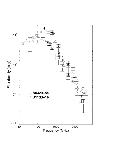
Figure 3: Spectra computed from equivalent continuum flux densities for B0329+54 (circles) and B1133+16 (triangles). The open symbols are values taken from the literature, while the filled symbols were derived from the single pulse measurements presented here.

While the average flux densities are consistent with the expected values, we correct for short term variation due to ISS according to the following scheme: We compute a 200-sec running median for the time series which we wish to correct. A time of 200 sec was chosen to be longer than intrinsic pulse-to-pulse modulation and to be smaller or of similar scale as the expected (diffractive and refractive) scintillation time scales (see Table 1). The flux density of each pulse is divided by this running median and the whole dataset is then rescaled to be consistent with the initial average flux density. According to the scintillation parameters summarized in Table 1, this procedure is mostly important for the 1412 MHz times series of both PSRs B0329+54 and B1133+16, as well as the 626 MHz time series of PSR B1133+16. As a detail, we note that any missing pulses due to the nulling phenomena (Backer 1970) observed in PSR B1133+16, which will be studied elsewhere (Bhat et al. in prep.), were replaced by a preceding detected pulse before computing the running median.

Table 3: Modulation indices for the variation in observed flux density caused by interstellar scintillation, $m_{\rm ISS}$, and intrinsic variation, $m_{\rm int}$

Frequency B0329+54 B1133+16 (MHz) $m_{\rm ISS}$ $m_{\rm int}$ $m_{\rm ISS}$ $m_{\rm int}$ 238 0.08 0.71 – – 341 – – 0.16 0.95 626 0.17 0.75 0.74 1.16 1412 0.31 0.44 0.98 1.21 4850 0.12 1.10 0.28 2.94

We can use the time series computed from the 200-sec running median to derive the modulation index defined in Eq. 2 as a result from intensity variation caused by interstellar scintillation, $m_{\rm ISS}$. Similarly, the left-over, short-term variations are a measure for the intrinsic pulse-to-pulse modulation, which we can express by a modulation index computed from the corrected time series, $m_{\rm int}$. Both sets of values are listed in Table 3.

While we would expect a modulation index of about unity in the strong scintillation regime, the actual observed ISS modulation will depend on the number of scintles sampled in time and frequency. In case of an observing bandwidth large compared to the scintle bandwidth, we can expect the modulation index to be reduced by a factor of approximately $1/\sqrt{n}$ where $n$ is the number of scintles averaged over. Indeed, our observations confirm this expected behaviour as can be seen for instance, for PSR B0329+54 at 238 MHz. Our bandwidth for this observation was about 1600 times the expected scintillation bandwidth (see Table 1), so that we would expect the modulation index to be only of the order of 0.03 (Table 3), which is close to the observed value after applying our correction scheme. For PSR B1133+16, the observing bandwidth at 326 MHz is about 16 times larger than the estimated scintillation bandwidth, and the expected modulation index of $1/\sqrt{16}=0.25$ is again close to what is observed.

The observations also confirm our earlier expectations that the data mostly affected by ISS are those at 1412 MHz and the PSR B1133+16 data at 626 MHz. While our observing time for PSR B0329+54 is not sufficient to fully sample the ISS variations at 1412 MHz in time, resulting in a modulation index of somewhat less than unity, the measured modulation index of PSR B1133+16 is indeed consistent with unity at that frequency, as expected. At 626 MHz, we would expect a modulation index of $1/\sqrt{16/11.4}=0.83$ (see Table 1) which is close to the 0.74 measured for PSR B1133+16. Moreover, both pulsars are clearly in the weak scintillation regime at 4850 MHz, and the derived modulation indices are consistent with those of Malofeev at el. (1996) obtained at the same frequency. We can therefore be assured that our procedure can successfully separate the modulations due to ISS from the intrinsic flux density variations.

After the correction scheme, which is equivalent to a high-pass filtering, we are left with the intrinsic flux density time series. Any possible imperfections of the scheme, such as unmodelled refractive scintillation, are accounted for by adopting uncertainties as derived in Sect. 3.1. We can therefore assume that our modulation indices, $m_{\rm int}$, describe intrinsic intensity variations. We can compare our $m_{\rm int}$ to those presented by Bartel et al. (1980). They studied the frequency dependence of the intrinsic pulse-to-pulse modulation for a large sample of pulsars, including PSRs B0329+54 and B1133+54. Interestingly, Bartel et al. found that $m_{\rm int}$ first decreases with frequency, before it starts to rise again beyond a critical frequency, $\nu_{\rm m}^{c}$, which they estimated to be $\nu_{\rm m}^{c}\sim 1400$ MHz for PSR B0329+54 and $\nu_{\rm m}^{c}\sim 600$ MHz for PSR B1133+16, respectively. We show the modulation indices presented by Bartel et al. (1980) together with our $m_{\rm int}$ measurements in Fig. 4. Indeed, our values agree well with the previous measurements, in particular when considering that our data have been taken simultaneously at different frequencies while those of Bartel et al. were compiled from different epochs. Moreover, both pulsars known to switch radiation patters; PSR B0329+54 shows a very prominent moding behaviour (e.g. Bartel et al. 1982), while PSR B1133+16 is a well known for its nulling phenomenon. It is likely that these phenomena have affected our analysis techniques and those of Bartel et al. (1980) differently, explaining some of the few differences. We note that our very high modulation index for PSR B1133+16 is probably related to another phenomenon, discussed in detail in Sect. 5.

Overall, it is worth emphasizing that the peculiar frequency behaviour of the pulse-to-pulse modulation index is supported by our measurements which were made simultaneously at the different frequencies.

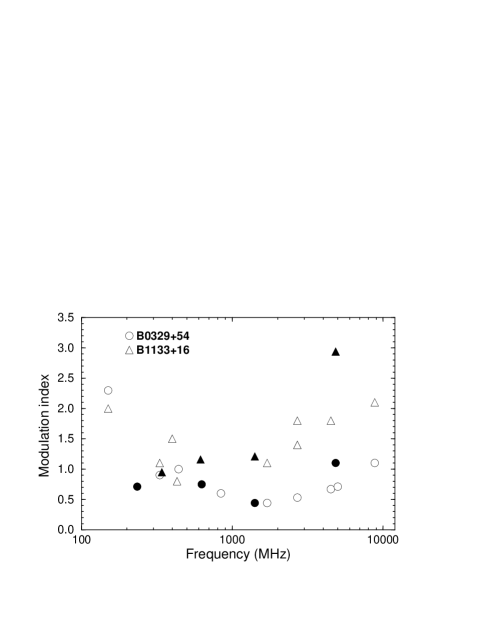
Figure 4: Intrinsic pulse-to-pulse modulation indices, $m_{\rm int}$ as presented by Bartel et al. (1980, open symbols) and as derived from our measurements (filled symbols). The peculiar frequency behaviour first pointed out by Bartel et al. (1980) is clearly visible.

4 Radio spectra of individual pulses

4.1 Correlations between frequencies

Using the ISS corrected flux densities, we can inspect the correlation of the intrinsic intensities between the different frequencies. Fig. 5 shows the flux densities measured at our four frequencies for PSR B0329+54. Corresponding correlation coefficients are summarized in Table 4. In order to estimate uncertainties in the correlation coefficients, we followed the example of Bhat (1998) and used the “boot-strap” method (e.g. Efron 1979, Press et al. 1992). We also produced simulated pulses with varying signal-to-noise ratio to study the effect of noise on the measured correlation coefficient (cf. Kardashev et al. 1986). We find that for our signal strengths, the reduction of the correlation coefficient is typically less than 5%. Hence, rather than trying to correct for this effect, a corresponding error was added in quadrature to the boot-strap uncertainties, resulting in the values shown in Table 4. Interestingly, the correlations are clearly tighter for adjacent frequency bands than for those widely separated. In fact, the best correlation can be observed between 626 and 1412 MHz, while the worst obviously exists for the 238/4850 MHz pair.

The average profile of pulsars can be separated into individual components that are well described by a Gaussian shape, for which a spectral behaviour can be determined (e.g. Kramer et al. 1994). Although this procedure should also be performed ideally when studying components of single pulses, this is difficult to achieve with single pulses which are not necessarily of Gaussian shape. In order to study the basic spectral behaviour of individual single pulse components, we instead define windows across the pulse for which we study the flux density separately. For PSR B0329+54 we choose the three windows as shown for the 1.41-GHz profile in Fig. 6. We are aware that this is only a crude approximation, as it has been shown that the profile consists of at least five (Kramer 1994) or even nine components (Gangadhara & Gupta 2001), but we believe that more complicated analysis will not alter the results significantly. We note that the windows chosen are adequate for the profiles at all frequencies. The correlation coefficients for these components separately are also given in Table 4. Obviously, the best correlation occurs for the central component, while the worst is present for trailing one. We can compare these results to those of Kardashev et al. (1986), who looked at phase-resolved correlation coefficients between widely-spaced frequencies. Even though we can expect our results to differ somewhat as we study only the correlation of the flux densities measured in a given, much wider window, rather than attempting a phased-resolved analysis as already done in the first paper of this series by Karastergiou et al. (2001), the results agree very well. Kardashev et al. studied pulses observed at 102.5 MHz and 1700 MHz and find correlation coefficients of about 0.38 and 0.43 for longitudes roughly situated within our windows C2 and C3. Given their much lower frequency of 102.5 MHz, their obtained values are in good agreement. It is difficult to judge the observation that their C3 value is larger than their value determined for C2, as they do not estimate uncertainties and as their C3 value is in fact smaller before a noise-correction is applied.

Figure 5: Correlation between the equivalent continuum flux densities observed for PSR B0329+54 simultaneously at four frequencies.

Figure 6: Average profile of PSR B0329+54 as observed at 1.41 GHz. The three designated windows are referred to as Component 1, 2 and 3.

Table 4: Correlation coefficients for PSR B0329+54 as determined from the equivalent continuum flux densities measured between frequency pairs for the full pulse and the components 1, 2 and 3. Uncertainties have been computed using the boot-strap method and simulated pulses (see text for details).

Freq.		626 MHz		1412 MHz		4850 MHz
238 MHz	Pulse	0.67$\pm$	0.03	0.48$\pm$	0.03	0.31$\pm$	0.03
	C1	0.60$\pm$	0.04	0.47$\pm$	0.04	0.15$\pm$	0.03
	C2	0.69$\pm$	0.04	0.54$\pm$	0.03	0.39$\pm$	0.03
	C3	0.43$\pm$	0.03	0.29$\pm$	0.02	0.26$\pm$	0.02
626 MHz	Pulse			0.79$\pm$	0.04	0.66$\pm$	0.04
	C1			0.68$\pm$	0.04	0.28$\pm$	0.03
	C2			0.83$\pm$	0.04	0.72$\pm$	0.04
	C3			0.58$\pm$	0.04	0.22$\pm$	0.02
1412 MHz	Pulse					0.78$\pm$	0.04
	C1					0.51$\pm$	0.04
	C2					0.79$\pm$	0.04
	C3					0.60$\pm$	0.04

The data obtained for PSR B1133+16 are shown in Fig. 7 whereas correlation coefficients computed as for PSR B0329+54 are summarized in Table 5. Again the least correlation is observed for the frequency pair with the widest separation. In order to study the behaviour of profile components, we again define pulse windows as shown for PSR B1133+16 in Fig. 8. These two components are also only an approximation, since Kramer (1994) showed that the central bridge emission should be modelled as a separate component, perhaps representing the graze of an inner cone in a nested cone structure. Generally, the correlation coefficients for the two profile components (again in brackets) are larger than that for the full profile. The only exception is for the correlation between 1412 MHz and 4850 MHz, where at both frequencies the leading component is heavily dominating. Again, our results are consistent with those by Kardashev et al. (1986) who also find the first component to be better correlated than the second. Manchester et al. (1989) looked at this pulsar at three different frequency pairs, i.e. 410–928 MHz, 410–5860 MHz and 928–5600 MHz, respectively. As Kardashev et al. (1986), they performed a phase-resolved correlation analysis, finding again a better correlation for the first component. While a proper comparison is difficult due to the difference in freqencies and the lack of estimated uncertainties, their C1 appears to show the least correlation between 928 and 5600 MHz, while C2 exhibits the lowest correlation coefficient for 410 and 5860 MHz. Some of this difference is most likely due to a frequency-selective nulling behaviour of this pulsar. We note that during our observations nulling did not always occur simultaneously at all four frequencies. As we will detail in Bhat et al., (in prep.), while the majority of nulls are broadband, a significant fraction of them occur only over a narrow frequency range.

Figure 7: Correlation between the equivalent continuum flux densities observed for PSR B1133+16 simultaneously at four frequencies.

Figure 8: Average profile of PSR B1133+16 as observed at 1.41 GHz. The two designated windows are referred to as Component 1 and 2.

Table 5: Correlation coefficients for PSR B1133+16 as determined from the flux densities measured between frequency pairs for the full pulse and the components 1 and 2.

Freq.		626 MHz		1412 MHz		4850 MHz
341 MHz	Pulse	0.72$\pm$	0.04	0.51$\pm$	0.03	0.31$\pm$	0.02
	C1	0.77$\pm$	0.04	0.57$\pm$	0.03	0.35$\pm$	0.04
	C2	0.76$\pm$	0.05	0.61$\pm$	0.04	0.32$\pm$	0.03
626 MHz	Pulse			0.73$\pm$	0.04	0.49$\pm$	0.04
	C1			0.78$\pm$	0.04	0.55$\pm$	0.05
	C2			0.74$\pm$	0.05	0.48$\pm$	0.04
1412 MHz	Pulse					0.74$\pm$	0.04
	C1					0.76$\pm$	0.05
	C2					0.69$\pm$	0.04

4.2 Single pulse spectra

It is clear from Fig. 3 that the radio spectrum of PSR B0329+54 exhibits a maximum at around 300 MHz, close to or even above our lowest observing frequencies. In order to compare the single pulse spectra to the average radio spectrum, we therefore will not include this frequency in the process of fitting a power law spectrum $S(\nu)\propto\nu^{\alpha}$ to the single pulse flux densities of this pulsar. The distribution of spectral indices using the full pulse window is presented in the top panel of Fig. 9, showing a Gaussian shape. In order to compute the mean spectral index from the individual fits to the single pulses, we weight each result by the reduced $\chi^{2}$-value obtained in each fit, hence greatly reducing the impact of possible bad fits. We obtain a mean spectral index of $\bar{\alpha}=-2.4\pm 0.1$, which is consistent with the spectral indices obtained from using the published flux densities in the same frequency range as well as using the values obtained from the average profiles of our observations (see Table 6). This result may be compared to the results of a dual-frequency observation of PSR B0329+54 made at 327 MHz and 2695 MHz by Bartel & Sieber (1978). Their spectral index distribution also shows a Gaussian shape, even though their lowest frequency is very close to the spectral turn-over. Due to the use of 327-MHz data, one would expect that their mean spectral index may be biased towards flatter spectra, but Bartel & Sieber adjusted their distribution to have the same median as the average pulse spectra, so that no detailed comparison is possible. Additionally, we note that they did not correct their data for ISS effects which they estimated to be small for this pulsar at their frequencies.

Figure 9: Top: Distribution of spectral indices obtained for single pulses of PSR B0329+54 using the full pulse. Bottom: Mean of the equivalent continuum flux density of pulses with a spectral index within an interval of 0.5.

Computing the spectra for the components shown in Fig. 6 from the flux densities of the average pulse profiles, we obtain the spectra shown in Fig. 10 where we again ignore the lowest frequency due to the presence of a spectral turn-over. In contrast to the general behaviour of pulsars (e.g. Rankin 1983, Lyne & Manchester 1988), the central component, Comp 2, does not exhibit the steepest spectrum. Kramer (1994) obtained the same result for the average profile using five Gaussian components in a more sophisticated analysis in a frequency range from 1410 MHz to 10550 MHz. Our inner component corresponds roughly to his central three components, for which we find an index of $-2.2\pm 0.1$ using his data. This is consistent with our result. However, while both his leading outer components have a steeper spectrum than the trailing ones, we observe the opposite with the steepest spectrum for C3. It is conceivable that the different frequency range covered is most likely responsible, indicating a possible break in the component spectra.

All obtained spectral indices are summarized in Table 6. We also list the results obtained from the $\chi^{2}$-weighted distributions of single pulse spectra which are shown in Fig. 11. The results are again consistent. Not surprisingly, the distribution of the central, dominating component shows the largest resemblance to the distribution of the full pulse. The distributions for the outer components are much wider. While these components are weaker, their spectra are still well defined. The mean errors of the spectral indices are similar for all three components, and we do not find any correlation between the goodness-of-fit, $\chi^{2}$, and the fitted spectral indices. Hence, we believe that the distributions are intrinsically wider. We will revisit this observation later in light of the result for PSR B1133+16 described in the following.

Figure 10: Component spectra for PSR B0329+54 using equivalent continuum flux densities as measured of the average profiles at each frequency.

Table 6: Spectral indices obtained for PSR B0329+54 in the frequency range from 600 to 4850 MHz. The results using the published flux densities are quoted in Col. 2, using the flux densities from the average profile in Col. 3 and the weighted mean values of the single pulse spectra in Col. 4. Corresponding medians are quoted in brackets.

	Published	Average	Single
Full pulse	$-2.51\pm 0.13$	$-2.4\pm 0.1$	$-2.4\pm 0.1$	($-2.44$)
Comp. 1	–	$-2.4\pm 0.2$	$-2.2\pm 0.1$	($-2.32$)
Comp. 2	–	$-2.4\pm 0.2$	$-2.3\pm 0.1$	($-2.40$)
Comp. 3	–	$-2.6\pm 0.2$	$-2.5\pm 0.1$	($-2.59$)

Figure 11: Distribution of spectral indices obtained for single pulses of PSR B0329+54 using the three pulse windows shown in Figure 8.

We repeat the same analysis for PSR B1133+16. Here all our observing frequencies are obviously beyond the low frequency turn-over, so that we perform a power law fit to all frequencies. As we will detail in Bhat et al. (in prep.), nulling does not occur simultaneously at all frequencies for this pulsar. We fit a power law if at least three frequencies show detections of pulses (or pulse components, respectively). The distribution for the full pulse profile is shown in the top panel of Fig. 12. The corresponding ($\chi^{2}$-weighted) mean spectral index (see Table 7) is somewhat steeper than that for the average profile. While the values are just consistent within the errors, we note that the single pulse distribution is not of Gaussian shape, as in the case for PSR B0329+54, but that it shows a tail towards flatter indices. Again, this is consistent with the results of a dual-frequency observation by Bartel & Sieber (1978) made at 327 MHz and 2695 MHz. Their spectral index distribution is shifted towards flatter spectra when compared to our results, but as mentioned before Bartel & Sieber adjusted their distribution to have the same median as the average pulse spectra (known at that time). Additionally, they did not correct for effects caused by ISS. Whilst no detailed comparison is therefore possible, the asymmetry in the distribution is striking.

Figure 12: Top: Distribution of spectral indices obtained for single pulses of PSR B1133+16 using the full pulse. Bottom: Mean of the equivalent continuum flux density of pulses with a spectral index within an interval of 0.5.

Using the average flux densities for the component windows (see Fig. 8), we obtain the spectra shown in Fig. 13. Corresponding spectral indices are listed in Table 7. The values are in very good agreement with the results obtained by Kramer (1994) using Gaussian components, indicating again the validity of our relatively crude approach of windowing.

The distributions of the spectral index obtained for each component from the single pulses are shown in Fig. 13 and corresponding numbers are listed in Table 7. It is interesting to note that the width of the spectral index distributions ($\Delta\alpha\approx 1$) is similar to that of the outer components of PSR B0329+54. All of them are so-called “conal” components (e.g. Rankin 1983, Lyne & Manchester 1988) which are viewed further away from the magnetic meridian. It has been shown that geometrical factors can severely affect the spectral index observed for a given profile component (Kramer et al. 1994, Sieber 1997) and it seems therefore possible that geometry can also affect the spectral index distribution of single pulses. Indeed, it is conceivable that the the wider spectral index distributions as well as the observed weaker correlations (between pairs of frequencies) for PSR B0329+54’s outer components (see previous section) may be caused by the same underlying effect. Future comparisons of more single pulse spectra of “core” and “conal” components will help answer this question.

For the trailing component of PSR B1133+16, the mean of the spectral index distribution is the same as for the average profile spectrum. This is not the case for the dominating leading component or the full pulse profile. It is not obvious why this should be expected, in particular as PSR B0329+54 behaved differently. We will explore the possible reason for this effect in the following section.

4.3 Spectral index vs. pulse strength

An obvious difference in the spectral index distributions for the single pulses of PSRs B0329+54 and B1133+16 is the asymmetry and deviation from a Gaussian shape in the case of PSR B1133+16. Constructing these histograms we lose information about the relative strength of the observed single pulses, which is, together with the relative occurrence of weak and strong pulses, nevertheless relevant for the formation of the average profile. In order to recover this information, we group the single pulses into intervals (bins) of spectral indices, computing the average flux density at all frequencies for a given spectral index bin. We present the results in the bottom panels of Figs. 9 and 12 where we show the mean flux density for a pulse of given spectral index interval. We note that their is often a wide scatter of flux densities within a spectral index bin. As a consequence, in few cases when the number of pulses for a given bin is small, the spectral index derived from these average flux densities shown in Figs. 9 and 12 may not be identical to the one of the associated spectral index bin. However, the trend, as confirmed by the computation of the medians of the flux densities, is clear.

As one can see, for PSR B1133+16 there is a strong tendency for steep spectrum pulses to be weaker than those with a flatter spectrum (Fig. 12). This trend is strongest for pulses at 4.85 GHz, while there is a less severe but still very significant dependence at 626 MHz and 1412 MHz. The curve at 340 MHz is relatively flat with a trend into the opposite direction. The overall trend only flattens out for those 5% of pulses with a spectral index greater than $-1$.

For PSR B0329+54 the behaviour is strikingly different. While the mean flux density only drops significantly at 4.85 GHz for those 2% of pulses with a spectral index steeper than $-3$, the curves are otherwise remarkably flat at all frequencies, in particular for the vast majority of the pulses in the centre of the spectral index distribution. This is even true for the lowest frequency of 238 MHz, which follows the curves of the other frequencies, even though we have seen that this frequency is below the spectral turn-over. This observation may provide an important clue in identifying the origin of the spectral turn-over.

For PSR B1133+16, Fig. 12 points to the existence of pulses that are much stronger than the average at 4.85 GHz, but not necessarily at the lowest frequencies, so that the overall spectrum of these pulses is flatter than the average. This then causes an asymmetry in the resulting spectral index distributions, as observed.

At high frequencies the pulse profile of PSR B1133+16 is dominated by the leading component, as is seen in the spectral indices of Table 7. At 10.55 GHz, the trailing component is almost undetectable, and at 32 GHz the pulse profile is represented by the leading component alone (Kramer et al. 1996). Hence, we can expect that the 4850 MHz data in Fig. 12 are dominated by the behaviour of component 1. Indeed comparing the mean flux density for pulses with a spectral index $\alpha<-2.5$ to that of pulses with $\alpha>-1.5$, we find $0.21\pm 0.01$ and $8.7\pm 0.5$ mJy, respectively. For the second component, the difference is very much smaller, i.e. $0.51\pm 0.01$ and $1.4\pm 0.1$ respectively, but the fact that there is a difference in these values at all helps in understanding the asymmetry also observed in the spectral index distribution for this component.

It is the combined effect of pulse strength and relative occurrence which produces the average profile at a given frequency. While we have studied these two aspects independently from each other, we can attempt to understand their relative importance by computing the mean pulse profiles for each spectral index bin. In order to facilitate the discussion we use coarse spectral index bins of $\alpha\leq-2.5$, $-2.5<\alpha\leq-1.5$ and $\alpha>-1.5$, respectively. The results are shown in Fig. 15 for all frequencies and for the spectral indices measured for the full pulse and component 1 and 2. This figure indeed confirms our previous considerations: The figures for the full pulse look very similar to those of component 1, as expected. At high frequencies the flat spectrum profiles are dominated by a very strong first component, while this effect gradually disappears towards lower frequencies. The figures for the second component shows the expected selection against strong and weak pulses at low and high frequencies.

We have to conclude from the above that there is a group of strong pulses occurring mostly at the longitudes of the first component, which appear to be much stronger than the average pulses.

Figure 13: Component spectra for PSR B1133+16 using equivalent continuum flux densities as measured of the average profiles at each frequency.

Table 7: Spectral indices obtained for PSR B1133+16 in the frequency range from 340 to 4850 MHz. The result using the published flux densities is quoted in Col. 2, using the flux densities from the average profile in Col. 3 and the mean value of the single pulse spectra in Col. 4. Corresponding medians are quoted in brackets.

	Published	Average	Single
Full pulse	$-1.89\pm 0.07$	$-1.8\pm 0.1$	$-2.0\pm 0.1$	($-2.08$)
Comp. 1	–	$-1.7\pm 0.1$	$-2.0\pm 0.1$	($-2.02$)
Comp. 2	–	$-2.1\pm 0.1$	$-2.1\pm 0.1$	($-2.23$)

Figure 14: Distribution of spectral indices obtained for single pulses of PSR B1133+16 using the two defined pulse windows.

4.4 “Giant pulses” in PSR B1133+16 ?

In order to study the occurrence of strong pulses for PSR B1133+16 and to compare this to PSR B0329+54, we compute the cumulative probability distribution of the single pulse flux densities, shown in Fig. 16 for all frequencies. Note that for PSR B1133+16 we again only include detected (i.e. non-nulling) pulses.

In these plots we indicate the mean flux density, $<\!S\!>$, measured at the given frequency by a dashed line and also show a dotted-dashed line marking a value of $10\times\!<\!S\!>$. While the single pulses of PSR B0329+54 are well below this threshold at all frequencies (i.e. no pulse is stronger than even 5 times the mean at any frequency), for PSR B1133+16 we observe a number of pulses at 4850 MHz which well exceed the corresponding value. We also observe a shift in the location of the $10\times<\!S\!>$-line from low to high frequencies relative to the cut-off of the distributions. Therefore, in contrast to PSR B0329+54, PSR B1133+16 has a significant fraction of strong pulses which appear to become more frequent towards higher frequencies.

Figure 15: Average pulse profiles of PSR B1133+16 computed for sets of pulses with spectral indices measured in the intervals $\alpha\leq-2.5$, $-2.5<\alpha\leq-1.5$ and $\alpha>-1.5$, respectively, for the whole profile and component 1 and 2. The y-axis shows corresponding peak flux densities.

In total we identify 40 pulses of PSR B1133+16 at 4850 MHz, whose mean flux density exceeds 10 times the mean. This threshold is commonly used to define so-called “giant pulses” which have been observed for the Crab pulsar, PSR B1937+21 and PSR B1821$-$24 (see Johnston & Romani 2002 for a recent review). In addition to their large mean flux density, giant pulses also show a power-law distribution in their energy distributions and tend to occur at a specific range of pulse phases. Giant pulses also appear to be broadband by exceeding the mean flux density by a factor of 10 or more at all frequencies. The latter point is mostly based on non-simultaneous observations by studying the energy distribution at different frequencies (e.g. Lundgren et al. 1995), but simultaneous dual-frequency observations have been made for the Crab pulsar (see Sallmen et al. 1999 and references therein) where only 70% of all giant pulses are seen both at 600 and 1400 MHz. The results of these studies for the spectral index of giant pulses are somewhat inconclusive. While earlier observations conclude that, on average, the spectral index of giant pulses is flatter than the average main pulse spectral index, this finding is not supported by the most recent study where the average spectral index of the giant pulses is comparable to that of the average main pulse (see discussion by Sallmen et al. 1999). However, the Crab pulsar has a very steep radio spectrum, so little may be learnt from the relative strength of its normal and giant pulses at either extreme end of the radio spectrum. However, we can compare other aspects of the strong pulses from PSR B1133+16 pulses to the known properties of giant pulses or those of so-called “giant micropulses”. The latter have been discovered for the Vela pulsar as very strong narrow pulses of very small width occurring at fixed, narrow phases (Johnston et al. 2001), also showing a power-law energy distribution.

While a power-law visible in the cumulative probability function of giant pulse flux densities clearly separates them from normal pulses, this appears not to be the case for PSR B1133+16 in Fig. 16. It is possible that a number of 40 “giant” pulses is too small to produce a recognisable feature, but a rate of one strong pulse in every 100 (at 4850 MHz) is a much higher rate than for PSRs B1821$-$24 and B1937+21 and is comparable to that of the Crab pulsar. The noticeable change in slope of the high energy end of PSR B1133+16’s cumulative probability functions, when going from low to high radio frequencies, may be an indication of an emerging power-law component.

It appears that the strong pulses in PSR B1133+16 preferably occur at the pulse phase of the leading component. This is verified by computing the average profile from the 40 strong pulses at 4850 MHz. This profile is shown as the inset to Fig. 17 where we compare it to the average pulse profile. It becomes obvious that the strong pulses appear to be narrower and indeed appear mostly at the trailing edge of the leading component, being slightly offset from its centre. This implies that any correlation in the flux densities of the two normal profile components should become weaker at higher frequencies, when the strong pulses in the leading component clearly dominate the energetics. That is indeed the case (see Fig. 18) where the flux densities appear almost anti-correlated at 4850 MHz. This observation also explains the fact mentioned in Sect. 4.1 that the correlation coefficient between frequency pairs are larger for each component separately than for the full profile.

We can study the broadband characteristics for PSR B1133+16 by inspecting our 40 strong pulses at the lower frequencies. The three strongest pulses are shown in Fig. 17. It turns out that 36 out of the 40 pulses are also much stronger than the average pulse at a given phase at the lower frequencies. But since the emission of these pulses is mostly concentrated in longitudes of the leading component, while the second component is significantly stronger at the lower frequencies, the mean flux density does not exceed the giant-pulse threshold at those. There are 4 pulses (or 10%), however, which do not appear to be broadband in their strength. One of those is shown in the same Figure.

Figure 16: Cumulative probability function of the single pulse equivalent continuum flux densities of PSR B0329+54 (left) and PSR B1133+16 (right). Frequencies 238 MHz, 626 MHz, 1412 MHz and 4850 MHz are shown from top to bottom. The dashed lines mark the mean of the equivalent continuum flux density at the given frequency, while the dot-dashed lines indicate 10 times the mean.

Based on the very small sample of pulsars known to exhibit giant pulses, it had been suggested that the occurrence of giant pulses may be related to the magnetic field strength at the light cylinder (e.g. Cognard et al. 1996) or to the emission process creating X-ray and gamma-ray emission (Johnston & Romani 2002). While PSR B1133+16 is not among the list of detected X-ray emitters, its magnetic field at the light cylinder is five orders of magnitude smaller than that of the Crab pulsar or PSR B1937+21. Overall, however, it seems possible that the strong pulses seen for PSR B1133+16 at 4850 MHz are a population of giant pulses which only manifest themselves at the higher frequencies because their radio spectrum is significantly flatter than that of the normal pulsar emission. This is consistent with observations of single pulses of PSR B1133+16 at an even higher frequency of 8450 MHz where the “giant” pulses appear even more frequently (Maron & Löhmer, private communication). Certainly, a classification as giant pulses cannot be based on the measured flux density alone (see also Johnston & Romani 2002), so that better statistics are needed to determine as to whether a power-law is present in their energy distribution to confirm their nature.

Figure 17: The three strongest pulses of PSR B1133+16 observed at 4850 MHz, showing simultaneously their occurrence at the lower frequencies. The average pulse profile (solid line) at these frequencies is also shown, multiplied by 50 at 4850 MHz and by 10 at the other frequencies. The y-axis shows corresponding peak flux densities. The inset in the lowest plot shows the average profile computed from the 40 “giant” pulses at 4850 MHz relative to the average pulse profile, multiplied by a factor of 20. One can see that the strong pulses tend to occur at the trailing edge of the leading component, being slightly offset from its centre.

Figure 18: Correlation of the equivalent continuum flux density of both components, C1 and C2, in PSR B1133+16 for all observed frequencies. While the correlation is generally weak, the components appear to be independent at the highest frequency.

5 Summary & Conclusion

Analysing simultaneous multi-frequency observations of PSRs B0329+54 and B1133+16 we have derived intrinsic flux density time series by correcting for scintillation effects. The resulting pulse-to-pulse modulation indices show a minimum around 1 GHz and increase above and below this frequency. This effect may be caused by a loss in coherence. Indeed, inspecting the correlations between the flux densities of different frequency pairs, it is striking that the correlation decreases as the frequency widens. Similar effects have been observed for the polarization properties in Karastergiou et al. (2001, 2002) and are clear indications for an intrinsic bandwidth of the emission process or propagation effects in the magnetosphere.

We determined the intrinsic flux density spectra for single pulses of PSR B0329+54 and derive similar conclusions as obtained from the average profiles. This suggest a relatively stable formation process of the average pulse profile, with spectral indices which are flatter for the central part than for the outer components. The distributions of spectral indices are wider for the outer conal component which are comparable in width to those of PSR B1133+16. This may be also related to the observation of weaker correlations observed for outer components of PSR B0329+54 and could be linked to a line-of-sight further away from the magnetic meridian. The flux densities below the spectral low-frequency turn-over seem to be still related to the spectrum and flux densities at the higher frequencies.

The spectral index distributions for the single pulses of PSR B1133+16 show significant deviations from a Gaussian shape. This asymmetry is caused by strong pulses which qualify as giant pulses according to their mean flux density at 4850 MHz. We have shown that most of these pulses are broadband and occur at a relatively narrow range of phases in the trailing edge of the leading component. All these properties suggest that these pulses may be indeed related to the giant-pulse phenomenon, whereas their relative spectral index is such that they only become dominant at the higher frequencies. However, a power-law behaviour in the energy distributions has not been observed yet and better statistics is required. Hence, the main conclusions of this paper are:

• The intrinsic pulse-to-pulse modulation has a minimum around 1 GHz.

• The correlations in flux densities between frequency pairs becomes weaker as the frequency separation widens. The best correlation is obtain between 600 and 1400 MHz, and it becomes worse for outer profile components.

• The distribution of spectral indices measured for single pulses of PSR B1133+16 is asymmetric (non-Gaussian), caused by a population of strong, flat-spectrum pulses.

• These strong pulses show a number of features which suggests their nature as giant pulses.

We have demonstrated that the study of the radio spectra of single pulses represents a so-far untapped reservoir of information directly related to the radiating particles and their emission process. Understanding their properties (unclouded by any averaging process) appears to be essential in the identification of the underlying emission process.

- (1) Backer, D. C. 1970, Nature, 228, 42
- (2) Backer, D. C., Fisher, J. R. 1974, ApJ, 189, 137
- (3) Bartel, N., Sieber, W. 1978, A&A, 70, 307
- (4) Bartel, N., Sieber, W., Wolszczan, A. 1980, A&A, 90, 58
- (5) Bartel, N., Morris, D., Sieber, W., Hankins, T.H. 1982, ApJ, 258, 776
- (6) Bhat, N.D.R. 1998, Ph.D. thesis, University of Pune
- (7) Bhat, N.D.R., Gupta, Y., Rao, P. 1999a, ApJ, 514, 249
- (8) Bhat, N.D.R., Rao, P., Gupta, Y. 1999b, ApJSS, 121, 483
- (9) Cognard, I., Shrauner, J. A., Taylor, J. H., Thorsett, S. E. 1996 ApJ, 457, L81
- (10) Cordes, J. M., Rickett, B. J. 1998, ApJ, 507, 846
- (11) Efron, B. 1979, Anns. Stat., 7, 1
- (12) Gupta, Y. 1995, ApJ, 451, 717
- (13) Gangadhara, R. T. and Gupta, Y. 2001, ApJ, 555, 31
- (14) Johnston, S., van Straten, W., Kramer, M., Bailes, M. 2001, ApJ, 549, L101
- (15) Johnston, S., Romani, R. 2002, MNRAS, 332, 109
- (16) Karastergiou, A., von Hoensbroech, A., Kramer, M. et al. 2001, A&A, 379, 270
- (17) Karastergiou, A., Kramer, M., Johnston, S. et al. 2002, A&A, 391, 247
- (18) Karastergiou, A., Johnston, S., Kramer, M. 2003, A&A, in press
- (19) Kardashev, N.S., Nikolaev, N. Ya., Novikov, A. Yu. P et al. 1986, A&A, 163, 114
- (20) Kondratiev, V. I., Popov, M. V., Soglasnov, V. A., Kostyuk, S. V. 2001, Astrophysics & Space Science, 278, 43
- (21) Kramer, M. 1994, A&AS 107, 527
- (22) Kramer, M., Wielebinski, R., Jessner, A. et al. 1994, A&AS, 107, 515
- (23) Kramer, M., Xilouris, K. M., Jessner, A. et al. 1996, A&A, 306, 867
- (24) Lorimer, D. R., Jessner, A., Seiradakis, J. H. et al. 1998, A&AS 128, 541
- (25) Lundgren, S., Cordes, J. M., Ulmer, M. et al. 1995, ApJ, 453, 433
- (26) Lyne, A.G., Manchester, R.N. 1988, MNRAS 234, 477
- (27) Malofeev, V. M., Shishov, V. I., Sieber, W. et al. 1996, A&A, 308, 180
- (28) Malofeev, V. M., Malov, I. F. 1980, Sov. Astron, 24, 54
- (29) Manchester, R.N., Popov, M.V., Soglasnov, V.A. 1989, Sov. Astron. Lett., 15, 43
- (30) Maron, O., Kijak, J., Kramer, M. et al. 2000, A&AS, 147, 195
- (31) Ott, M., Witzel A., Quirrenbach A. et al. 1994, A&A, 284, 331
- (32) Peng, B., Kraus, A., Krichbaum, T.P., Witzel, A. 2000, A&AS, 145, 1
- (33) Press, W. H., Teukolsky, S. A., Vetterling, W. T., Flannery, B. P. 1992, Numerical Recipes: The Art of Scientific Computing, 2nd edition, Cambridge University Press, Cambridge
- (34) Rankin, J. M. 1983, ApJ, 274, 358
- (35) Rickett, B. J. 1990, ARAA, 28, 561
- (36) Robinson, B.J., Cooper, B.F.C., Gardner, F.F. et al. 1968, Nature, 218, 1143
- (37) Sallmen, S., Backer, D. C., Hankins, T. H. et al. 1999, ApJ, 517, 460
- (38) Sieber, W. 1982, A&A, 113, 311
- (39) Sieber, W. 1997, A&A, 321, 519
- (40) Stinebring, D. R., Condon, J.J. 1990, ApJ, 352, 207
- (41) Stinebring, D. R., Faison, M. D., McKinnon, M. M. 1996, ApJ, 460, 460
- (42) Stinebring, D. R., Smirnova, T. V., Hankins, T. H. et al. 2000, ApJ, 539, 300