High resolution simulations of nonhelical MHD turbulence

Abstract

According to the kinematic theory of nonhelical dynamo action the magnetic energy spectrum increases with wavenumber and peaks at the resistive cutoff wavenumber. It has previously been argued that even in the dynamical case the magnetic energy peaks at the resistive scale. Using high resolution simulations (up to $1024^{3}$ meshpoints) with no large scale imposed field we show that the magnetic energy peaks at a wavenumber that is independent of the magnetic Reynolds number and about 5 times larger than the forcing wavenumber. Throughout the inertial range the spectral magnetic energy exceeds the kinetic energy by a factor of 2 to 3. Both spectra are approximately parallel. The total energy spectrum seems to be close to $k^{-3/2}$, but there is a strong bottleneck effect and it is suggested that the asymptotic spectrum is instead $k^{-5/3}$. This is supported by the value of the second order structure function exponent that is found to be $\zeta_{2}=0.70$, suggesting a $k^{-1.70}$ spectrum. The third order structure function scaling exponent is very close to unity, in agreement with Goldreich-Sridhar theory.

Adding an imposed field tends to suppress the small scale magnetic field. We find that at large scales the magnetic power spectrum follows then a $k^{-1}$ slope. When the strength of the imposed field is of the same order as the dynamo generated field, we find almost equipartition between the magnetic and kinetic power spectra.

guessConjecture

1 Introduction

Magnetic fields may play an important role during star formation. Stars are generally formed in strongly magnetized regions, and the magnetic pressure that builds up in shocks and the initial collapse is likely to determine the detailed evolution.

Early simulations of hydromagnetic turbulence have always suggested that the magnetic field is more intermittent than the velocity field if the field is generated by dynamo action [Meneguzzi et al. (1981), Kida et al. (1991)]. Furthermore, linear theory [Kazantsev (1968)] suggests that the magnetic spectrum should peak at the resistive scale, and it has been argued that this may hold even in the nonlinear regime [Maron & Blackman (2002)].

On the other hand, if there is an imposed large scale field there is no doubt that most of the magnetic energy resides at large scales e.g. Cho & Vishniac (2000). The obvious question is therefore, is it really true that the cases of dynamo-generated and imposed fields are indeed drastically different?

The purpose of this paper is to compare the case of an imposed field with that of a dynamo-generated one. We begin by briefly reviewing the main results of our recent paper [Haugen et al. (2003)] where we show that in the dynamo case the magnetic energy does not peak at the resistive scale.

2 Equations

Our approach is the same as in Haugen et al. (2003), which is similar to that of Brandenburg (2001), except that the flow is now forced without helicity. We adopt an isothermal equation of state with a constant sound speed $c_{\rm s}$, so the pressure $p$ is related to the density $\rho$ by $p=\rho c_{\rm s}^{2}$. The equation of motion is written in the form

$${{\rm D}{}\mathchoice{\mbox{\boldmath$\displaystyle u$}}{\mbox{\boldmath$\textstyle u$}}{\mbox{\boldmath$\scriptstyle u$}}{\mbox{\boldmath$\scriptscriptstyle u$}}{}\over{\rm D}{}t}=-c_{\rm s}^{2}\mathchoice{\mbox{\boldmath$\displaystyle\nabla$}}{\mbox{\boldmath$\textstyle\nabla$}}{\mbox{\boldmath$\scriptstyle\nabla$}}{\mbox{\boldmath$\scriptscriptstyle\nabla$}}{}\ln\rho+{\mathchoice{\mbox{\boldmath$\displaystyle J$}}{\mbox{\boldmath$\textstyle J$}}{\mbox{\boldmath$\scriptstyle J$}}{\mbox{\boldmath$\scriptscriptstyle J$}}{}\times\mathchoice{\mbox{\boldmath$\displaystyle B$}}{\mbox{\boldmath$\textstyle B$}}{\mbox{\boldmath$\scriptstyle B$}}{\mbox{\boldmath$\scriptscriptstyle B$}}{}\over\rho}+\mathchoice{\mbox{\boldmath$\displaystyle F$}}{\mbox{\boldmath$\textstyle F$}}{\mbox{\boldmath$\scriptstyle F$}}{\mbox{\boldmath$\scriptscriptstyle F$}}{}_{\rm visc}+\mathchoice{\mbox{\boldmath$\displaystyle f$}}{\mbox{\boldmath$\textstyle f$}}{\mbox{\boldmath$\scriptstyle f$}}{\mbox{\boldmath$\scriptscriptstyle f$}}{},$$ (1)

where ${\rm D}{}/{\rm D}{}t=\partial/\partial t+\mathchoice{\mbox{\boldmath$\displaystyle u$}}{\mbox{\boldmath$\textstyle u$}}{\mbox{\boldmath$\scriptstyle u$}}{\mbox{\boldmath$\scriptscriptstyle u$}}{}\cdot\mathchoice{\mbox{\boldmath$\displaystyle\nabla$}}{\mbox{\boldmath$\textstyle\nabla$}}{\mbox{\boldmath$\scriptstyle\nabla$}}{\mbox{\boldmath$\scriptscriptstyle\nabla$}}{}$ is the advective derivative, $\mathchoice{\mbox{\boldmath$\displaystyle J$}}{\mbox{\boldmath$\textstyle J$}}{\mbox{\boldmath$\scriptstyle J$}}{\mbox{\boldmath$\scriptscriptstyle J$}}{}=\mathchoice{\mbox{\boldmath$\displaystyle\nabla$}}{\mbox{\boldmath$\textstyle\nabla$}}{\mbox{\boldmath$\scriptstyle\nabla$}}{\mbox{\boldmath$\scriptscriptstyle\nabla$}}{}\times\mathchoice{\mbox{\boldmath$\displaystyle B$}}{\mbox{\boldmath$\textstyle B$}}{\mbox{\boldmath$\scriptstyle B$}}{\mbox{\boldmath$\scriptscriptstyle B$}}{}/\mu_{0}$ is the current density, $\mu_{0}$ is the vacuum permeability, $\mathchoice{\mbox{\boldmath$\displaystyle F$}}{\mbox{\boldmath$\textstyle F$}}{\mbox{\boldmath$\scriptstyle F$}}{\mbox{\boldmath$\scriptscriptstyle F$}}{}_{\rm visc}$ is the viscous force, and $\textstyle f$ is a random forcing function that consists of non-helical plane waves. The continuity equation is written in terms of the logarithmic density,

$${{\rm D}{}\ln\rho\over{\rm D}{}t}=-\mathchoice{\mbox{\boldmath$\displaystyle\nabla$}}{\mbox{\boldmath$\textstyle\nabla$}}{\mbox{\boldmath$\scriptstyle\nabla$}}{\mbox{\boldmath$\scriptscriptstyle\nabla$}}{}\cdot\mathchoice{\mbox{\boldmath$\displaystyle u$}}{\mbox{\boldmath$\textstyle u$}}{\mbox{\boldmath$\scriptstyle u$}}{\mbox{\boldmath$\scriptscriptstyle u$}}{},$$ (2)

and the induction equation is solved in terms of the magnetic vector potential $\textstyle A$, where $\mathchoice{\mbox{\boldmath$\displaystyle B$}}{\mbox{\boldmath$\textstyle B$}}{\mbox{\boldmath$\scriptstyle B$}}{\mbox{\boldmath$\scriptscriptstyle B$}}{}=\mathchoice{\mbox{\boldmath$\displaystyle\nabla$}}{\mbox{\boldmath$\textstyle\nabla$}}{\mbox{\boldmath$\scriptstyle\nabla$}}{\mbox{\boldmath$\scriptscriptstyle\nabla$}}{}\times\mathchoice{\mbox{\boldmath$\displaystyle A$}}{\mbox{\boldmath$\textstyle A$}}{\mbox{\boldmath$\scriptstyle A$}}{\mbox{\boldmath$\scriptscriptstyle A$}}{}$, so

$${\partial\mathchoice{\mbox{\boldmath$\displaystyle A$}}{\mbox{\boldmath$\textstyle A$}}{\mbox{\boldmath$\scriptstyle A$}}{\mbox{\boldmath$\scriptscriptstyle A$}}{}\over\partial t}=\mathchoice{\mbox{\boldmath$\displaystyle u$}}{\mbox{\boldmath$\textstyle u$}}{\mbox{\boldmath$\scriptstyle u$}}{\mbox{\boldmath$\scriptscriptstyle u$}}{}\times\mathchoice{\mbox{\boldmath$\displaystyle B$}}{\mbox{\boldmath$\textstyle B$}}{\mbox{\boldmath$\scriptstyle B$}}{\mbox{\boldmath$\scriptscriptstyle B$}}{}+\eta\nabla^{2}\mathchoice{\mbox{\boldmath$\displaystyle A$}}{\mbox{\boldmath$\textstyle A$}}{\mbox{\boldmath$\scriptstyle A$}}{\mbox{\boldmath$\scriptscriptstyle A$}}{},$$ (3)

where $\eta=\mbox{const}$ is the magnetic diffusivity. We use periodic boundary conditions in all three directions for all variables.

The solutions are characterized by the kinetic and magnetic Reynolds numbers,

$$\mbox{Re}=u_{\rm rms}/(\nu k_{\rm f}),\quad R_{\rm m}=u_{\rm rms}/(\eta k_{\rm f}),$$ (4)

respectively. The ratio of the two is the magnetic Prandtl number,

$$P_{\rm m}=\nu/\eta=R_{\rm m}/\mbox{Re}.$$ (5)

We use the Pencil Code which is a cache and memory efficient grid based high order code (sixth order in space and third order in time) for solving the compressible MHD equations.

3 Results

3.1 The peak of the magnetic power spectrum

Figure 1: Left: Magnetic power spectra for all our runs. We see that the peak of the magnetic power spectrum is at $k=5$ for all Re. Right: The peak of $B_{{\rm rms},l^{2}}$ is found at $k\approx 9$.

We have run simulations with up to $1024^{3}$ meshpoints in order to show that the magnetic energy spectrum does not peak at the resistive scale, as has previously been claimed [Maron & Blackman (2002)]. In the left panel of figure 1 we see that the peak of the spectrum is around $k=5$ for all our runs, i.e. it is independent of Re. We also note that we find a $k^{1/3}$ slope for small values of $k$ [Batchelor (1950)].

A more stringent measure is to look at the magnetic energy per unit logarithmic wavenumber interval, $kE_{M}(k)$, which would be flat if the contributions from small and large wavenumbers was equal. This is shown in the right hand panel of figure 1. We see that the peak of $kE_{M}(k)$ is shifted toward smaller scales compared to $E_{M}(k)$, but it is still not at the resistive scale. We do indeed see that for the largest runs it seems to settle at $k\approx 10$, which is well within the inertial range.

3.2 The inertial range

Figure 2: Kinetic and magnetic power spectrum of our largest run with $1024^{3}$ mesh points.

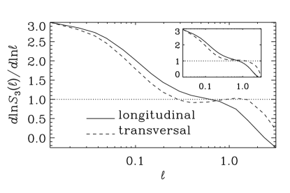
Figure 3: Left: logarithmic derivative of third order structure function. The inset is for a run with $256^{3}$ mesh points, while the large plot is for a run with $512^{3}$ mesh points. The result is consistent with $\zeta_{3}=1$ Right: logarithmic derivative of fourth order structure function. We see that this is clearly not compatible with $\zeta_{4}=1$

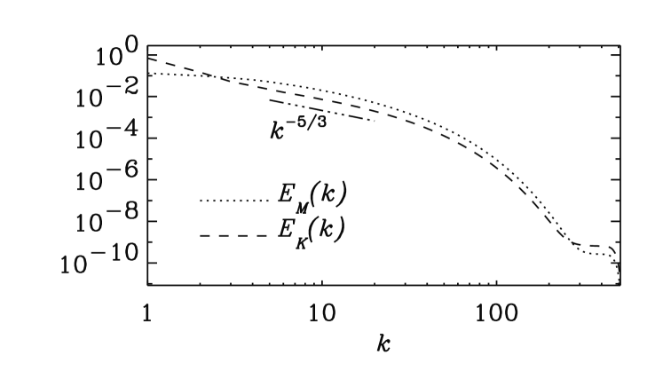
Figure 4: one-dimensional power spectra of our largest run. We see here that the inertial range is consistent with a $k^{-5/3}$ slope.

In figure 2 we see that there seem to be a clear inertial range for $7\lesssim k\lesssim 25$ where $E_{M}(k)$ and $E_{K}(k)$ are parallel and have a slope of $k^{-3/2}$. The $k^{-3/2}$ slope is suggestive of the Iroshnikov (1963) & Kraichnan (1965) (IK) theory, and may seem incompatible with the Goldreich & Sridhar (1995) (GS) theory. We also note that in the inertial range the fraction of the magnetic and kinetic energy seem to be saturated at; $E_{M}(k)/E_{K}(k)\approx 2.3$.

Knowing that IK theory predicts that the fourth order structure function scales linearly, while GS theory predicts linear scaling for the third order structure function, we now calculate the logarithmic derivatives for these structure functions; see figure 3. From these plots we see that the IK theory cannot be correct since the fourth order structure function is clearly steeper than linear. The third order structure function on the other hand scales linearly.

The second order structure function scaling exponent of the Elsasser variable, $\mathchoice{\mbox{\boldmath$\displaystyle z$}}{\mbox{\boldmath$\textstyle z$}}{\mbox{\boldmath$\scriptstyle z$}}{\mbox{\boldmath$\scriptscriptstyle z$}}{}^{\pm}=\mathchoice{\mbox{\boldmath$\displaystyle u$}}{\mbox{\boldmath$\textstyle u$}}{\mbox{\boldmath$\scriptstyle u$}}{\mbox{\boldmath$\scriptscriptstyle u$}}{}\pm\mathchoice{\mbox{\boldmath$\displaystyle B$}}{\mbox{\boldmath$\textstyle B$}}{\mbox{\boldmath$\scriptstyle B$}}{\mbox{\boldmath$\scriptscriptstyle B$}}{}/\sqrt{\rho\mu}$, is also indicative of GS theory being applicable since we find $\zeta_{2}=0.7$, which imply $E_{T}(k)=E_{M}(k)+E_{K}(k)\propto k^{-(1+\zeta_{2})}=k^{-1.7}$.

As we have argued earlier [Haugen et al. (2003)], the reason that figure 2 shows a $k^{-3/2}$ inertial range is that there is a strong bottleneck effect [Falkovich (1994)]. It turns out that this bottleneck is much stronger in three-dimensional power spectra than in one-dimensional ones [Dobler et al. (2003)]. We therefore plot in figure 4 the one-dimensional counterpart of figure 2 in figure 4. Here we see that the inertial range does indeed has a slope close to $-5/3$, as suggested by our previous findings from the structure functions. From this we conclude that also the three-dimensional power spectra will show a $k^{-5/3}$ inertial range away from the diffusive subrange.

3.3 Imposed magnetic field

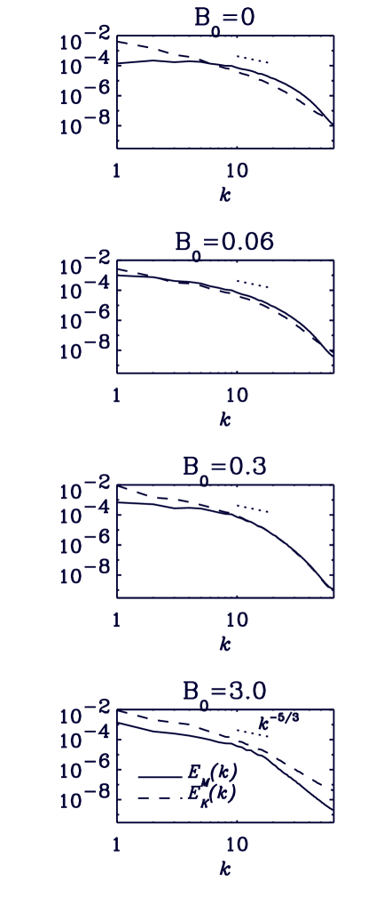
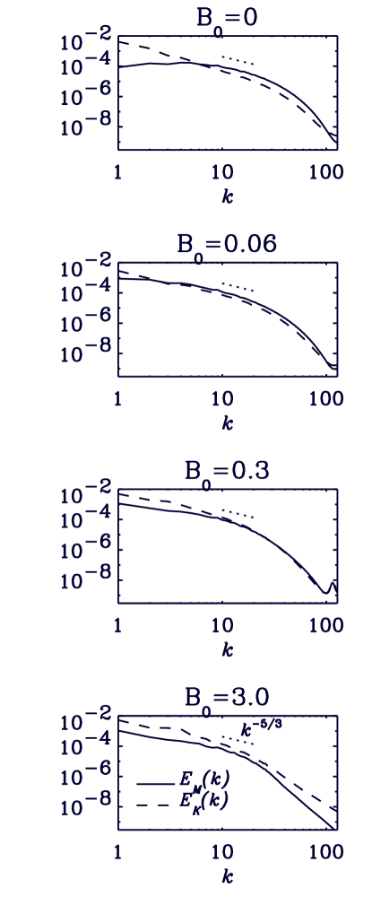
Figure 5: Left: power spectra for simulations with imposed fields of different strengths. $128^{3}$ meshpoints. Right: power spectra for simulations with imposed fields of different strengths. $256^{3}$ meshpoints.

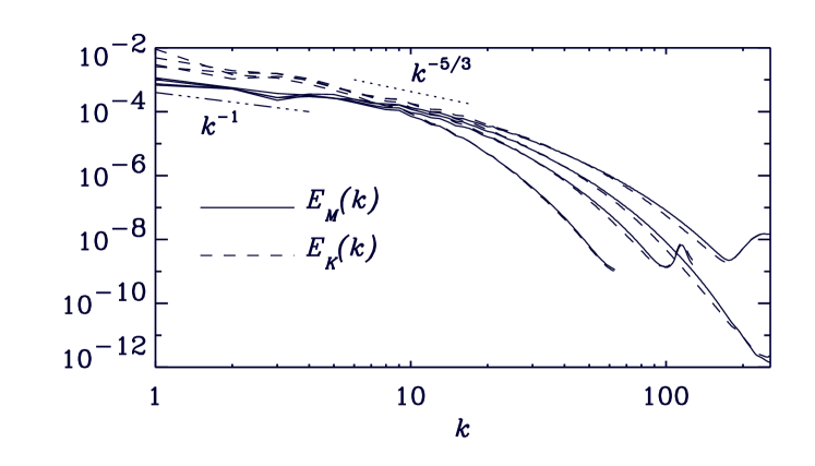
Figure 6: Power spectra for runs with different Re, and with $B_{0}=0.3$. We see a $k^{-1}$ for for $1<k<4$, and we also start to see the appearance of an $k^{-5/3}$ inertial range beginning at $k\approx 8$.

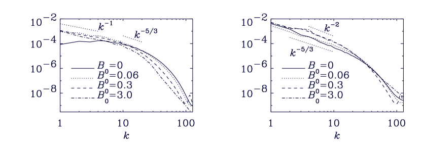
Figure 7: Power spectra for runs with different imposed fields. Left: magnetic power spectra; we see that the the larger the external field the more the magnetic field at small scales is suppressed. Right: kinetic power spectra

Until now we have only been looking at the case with no externally imposed field. We therefore want to see what effect such imposed fields of varying strengths have on the dynamo. In figure 5 we plot power spectra for simulations with $128^{3}$ meshpoints (left panel) and $256^{3}$ meshpoints (right panel) for different imposed fields. From the figure we see that having an imposed field seems to increase the large scale magnetic field at the same time as it decreases the small scale field. The stronger the external field the more suppressed are the small scale fields. We also note that with an imposed field the peak of the magnetic energy is found at the largest scale $(k=1)$, not at $k=5$ as in the case without an imposed field. Looking at figure 6 we see that for $1<k<4$ there seems to be a $k^{-1}$ slope for $E_{M}(k)$. Such a slope for the large scale magnetic field has been suggested previously [Ruzmaikin & Shukurov (1982), Kleeorin & Rogachevskii (1994), Brandenburg et al. (1996), Matthaeus & Goldstein (1986)]. From $k\approx 6$ there seems to be a short inertial range with a $k^{-5/3}$ slope, as expected from GS theory.

When the strength of the imposed field is comparable to the dynamo generated field ($B_{0}=0.06$ and $B_{0}=0.3$ in figure 5) we see that there is almost equipartition between magnetic and kinetic energy spectra, at least for the smaller scales. On the other hand, Cho & Vishniac (2000) find almost perfect equipartition for all scales. The difference is small, and could perhaps be explained by a difference in the forcing function. We did check, however, that changing from a delta-correlated forcing function to one with a renewal time comparable to the turnover time does not resolve this relatively minor discrepancy.

4 Discussion

We have shown that for non helical MHD turbulence without imposed magnetic field, $E_{M}(k)$ and $kE_{M}(k)$ peak at $k=5$ and $k=10$, respectively, and not at the resistive scale. We also find that in the inertial range $E_{M}(k)$ and $E_{K}(k)$ are parallel to each other, but with $E_{M}(k)/E_{K}(k)\approx 2.5$ and a slope of $k^{-5/3}$.

If we impose an external large scale field we find that $E_{M}(k)$ peaks at the box scale, and shows a $k^{-1}$ subinertial range. In the inertial range we find the expected $k^{-5/3}$ slope and almost equipartition between the kinetic and magnetic power spectra, i.e. $E_{M}(k)/E_{K}(k)\approx 1$, when the imposed field has a strength in the order of the dynamo generated field. An imposed large scale magnetic field therefore has the effect of increasing the magnetic energy at large scales, but decreasing it at small scales.