Ringing effects reduction by improved deconvolution algorithm

We develop a self-consistent automatic procedure to restore informations from astronomical observations. It relies on both a new deconvolution algorithm called LBCA (Lower Bound Constraint Algorithm) and the use of the Wiener filter. In order to explore its scientific potential for strong and weak gravitational lensing, we process a CFHT image of the galaxies cluster Abell 370 which exhibits spectacular strong gravitational lensing effects. A high quality restoration is here of particular interest to map the dark matter within the cluster. We show that the LBCA turns out specially efficient to reduce ringing effects introduced by classical deconvolution algorithms in images with a high background. The method allows us to make a blind detection of the radial arc and to recover morphological properties similar to those observed from HST data. We also show that the Wiener filter is suitable to stop the iterative process before noise amplification, using only the unrestored data .

1 Introduction

Despite its oustanding image quality, the small field of view of the Hubble Space Telescope (HST) still hampers its use for deep surveys covering angular size beyond a degree scale. Wide field surveys, like those used for gathering large sample of lensing clusters or for cosmic shear, are therefore a specific territory for panoramic CCD cameras, like Megacam at CFHT [Boulade et al. (2000)] or Omegacam at ESO [Valentijn et al. (2001)]. However, the intrinsic limitation of ground-based telescopes produced by atmospheric seeing puts severe bounds on the detection limits of these surveys and on the lowest gravitational distortion amplitude one can measure with these cameras. Image degradation dilutes the light from small faint galaxies below the limiting threshold, blurs image details and increases the uncertainties on shape measurement of lensed galaxies. Both arc detection and cosmic shear signal are therefore altered by the seeing.
Improving image quality from ground based telescopes is therefore an important technical goal that may have a significant scientific impact when surveys are pushed to the limits. In principle, image deconvolution can both improve the image quality and enhance the flux emitted by low surface brightness galaxies. Unfortunately, because deconvolution is a slow process and often produces unwanted artifacts, like ringing, it cannot be easily used on wide field ground based images. Furthermore, in the case of very large data sets from panoramic cameras, objective convergence criteria must be defined and applied automatically to images. These technical limitations turn out to be challenging if one envisions a massive image deconvolution of surveys.
Although it is not yet applicable to large ground based data sets, we explore new image deconvolution techniques that could be used in the future. More precisely, we compare the performances of the Richardson-Lucy (RL) algorithm with a modified version called the Lower Bound Constraint Algorithm (LBCA) that has been developped in [Lantéri et al. (2001)]. This algorithm, as well as the RL algorithm, shows noise amplification when the iteration number increases too much. A procedure to control automatically the iteration has then been implemented and validated on real data. It uses a HST image as a reference to stop the deconvolution process when a given distance between the HST image and the restored image is minimum. We choose to minimize an Euclidean distance criterion. This minimization technique also enables us to check the quality of the restoration.
Although the comparison with HST data turns out to be a successful way to test the method, it is unpractical for most images. Operating cosmological surveys will provide a huge amount of data that must be automatically processed, without any reference images. So, we generalized our empirical convergence criterion using the HST images to develop a systematic procedure to stop the deconvolution algorithm. This technique is based on the Wiener filtering and relies on the information contained in the data only.
In this first paper, we applied the deconvolution on CFHT images of the famous giant arc in Abell 370 and compare the result to HST data. Both the CFHT and the HST images are described in section 2. We determine the Point Spread Function (PSF) in the CFHT image in section 3 and apply the deconvolution techniques in section 4. We show that the LBCA must be preferred to the standard RL algorithm. In section 5, we use the technique based on the Wiener filter to stop the LBCA iterations without the need of any reference image. We show that the quality of the restored image then obtained with this independent procedure is satisfactory. We sum up our conclusions in section 6.

2 The data

Abell 370 is the most distant cluster of galaxies in the Abell catalogue, at a redshift z = 0.374 [Sarazin et al. (1982)]. The cluster structure is dominated by two giant elliptical galaxies, identified as $\#20$ and $\#35$ from the notations in [Soucail et al. 1987 b) ]. The image of Abell 370 exhibits a giant arc extending over 60 arc-second wide discovered by Soucail et al. [Soucail et al. 1987 a) ] and [Lynds & Petrosian (1986)]. This arc has been identified as an extremely distorted image of a background galaxy at z=0.724 [Soucail et al. (1988)], thus bringing the evidence of a cosmological gravitational lensing effect. The arc is split into five distinct regions $\#b$, $\#c$, $\#g$, $\#37$ and $\#62$ (see Fig. 6. in the present paper) and shows an intensity breaking between the galaxies $\#37$ and $\#62$. The galaxies $\#37$ ($z_{\#37}=0.37$), $\#b$ ($z_{\#b}=0.363$) and $\#c$ ($z_{\#c}=0.373$) are superimposed to the arc. On the contrary, the object $\#62$ belongs to it. The detection of a weak radial arclet in a HST/WFPC1 image (noted R) has been reported in [Smail et al. (1996)]. Its existence was confirmed in [Bézecourt et al. (1999)] who argued its redshift should be about 1.3. The detection of arclets, as well as the determination of sub-structures in the giant arc, are important to constrain the mass profile of Abell 370 as well as to scale its absolute mass.

2.1 CFHT observations of A370

The A370 image was obtained at the 3.60m telescope of the CFHT (Canada France Hawaï Telescope) observatory in November 1991 (see [Kneib et al. (1993)] for details). The FOCAM (Faint Object CAMera) imager installed on the prime focus of the telescope uses the filter $\#$1808 centered on 832 nm with a width of 196 nm. This image is integrated over 1800 seconds and corrected with standard CCD frame packages. The field extends over about 6x6 arc-minutes (’), with a sampling of 0.206 arc-second per pixel. The objects of specific interest correspond to the strong lensing effects observed close to the central galaxy ($\#$ 35 on Fig. 1 a). Thus we extract a sub-image extending over 0.6’ $\times$ 0.6’ approximately centered on this galaxy (image 196$\times$196 pixels).

2.2 HST observations of A370

We also have an A370 image with 622 seconds of integration time obtained with the HST in a wavelength domain close to the CFHT observations (F675W filter centered on $\lambda$=673,5 nm and width of 88,9 nm). The WFPC2 (Wide Field Planetary Camera 2) gives a wide field about 150 $\times$ 150 arcsec ($"$). We have extracted a region of about 34 $\times$ 34 $"$ (0,1”/pixel) containing the region of the giant arc. The high spatial resolution of the HST allows to observe details invisible in the CFHT image as sharp breakings in the giant arc and the presence of the radial arc $R$. We make the assumption that the HST image can be used as a reference for comparison with the restored image, i.e. we neglect any alteration induced from the HST instrument. We cannot exclude differences between the two original astronomical fields, because they are seen through different filters, but these differences are probably negligible for the study undergone here. This assumption is also supported by a mere visual inspection of the two images.

2.3 Comparison between HST and CFHT observations

The direct comparison between CFHT and HST images requires a linear transformation of the HST image since both orientation and spatial sampling are different. Let $(x^{\prime},y^{\prime})$ and $(x,y)$ be the spatial coordinates of a star photocenter in the HST and CFHT images respectively. The linear transformation between $(x^{\prime},y^{\prime})$ and $(x,y)$ may be written as:

$$\left\{\begin{array}[]{l}x^{\prime}=a.x+b.y+c\\ y^{\prime}=d.x+e.y+f\end{array}\right.$$ (1)

where $a$, $b$, $c$, $d$, $e$ and $f$ are unknown scalars. We then compute the linear transformation of the HST image with a bilinear interpolation. Solving the system (1) for a set of stars both identified in the CFHT and the HST 196$\times$196 sub-images, allows an accurate determination of the scalars $a$, $b$, $c$, $d$, $e$ and $f$. The comparison between the CFHT image and the transformed HST one is presented in Fig. 1.

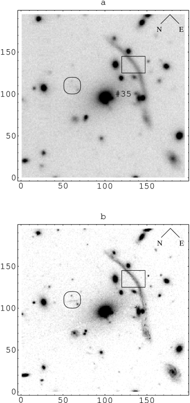
Figure 1: a) Extraction of a sub-image ($196\times 196$ pixels) of Abell 370 observed with the CFHT. The circle represents the region where the radial arc $R$ must be located.
The rectangular box ($20\times 28$ pixels) represents the mask used for the comparison of the two images in the case of the arc reconstruction.
b) Extraction of a sub-image ($196\times 196$ pixels) of Abell 370 image obtained by applying the linear transformation (1) on the HST image. The circle identifies the radial arc $R$.

The transformation (1) may be interpreted as a combination of a 110^∘ rotation followed by a 2.07 pixels dilatation from the center of the galaxy $\#$35 and a translation.

3 The Point Spread Function (PSF)

Ground-based observations suffer degradations due to the transmission of light by the atmosphere and the optics. The images obtained are then blurred by the system atmosphere-instrumentation. The field of the CFHT image extends over a few arc-minutes and corresponds to a long exposure time. In these conditions we can make the assumption that the degradation due to the atmosphere is space invariant in the image plane. Such an assumption is also safe for the instrumental distortions. The relation between the noiseless image $\tilde{y}(r)$ and the object $x(\alpha)$ is then a convolution one:

$$\tilde{y}(r)=\int_{-\infty}^{+\infty}h(r-\alpha)x(\alpha)d\alpha=h(r)\odot x(r)$$ (2)

where $r$ is the spatial coordinates at the telescope focus and $h$ the kernel of the integral equation (2) is the PSF of the system atmosphere-telescope.
The discretization of equation (2) leads to the matrix relation:

$$\tilde{y}=Hx$$ (3)

where $\tilde{y}$ is a vector corresponding to the noiseless image, $x$ a vector corresponding to the object and $H$ a matrix representing the convolution effects of the PSF. In real cases, the observations $y$ are a noise corrupted version of $\tilde{y}$. In all what follows, we assume a Poisson noise process.
The restoration technique we propose in this paper are then based on the deconvolution of the noisy image $y$ by an estimated PSF in order to reconstruct the object $x$ in the best conditions.

The first step consists in estimating the PSF from the stars (unresolved objects) in the full CFHT image.

3.1 Stars selection

We first identify the stars by using SExtractor [Bertin & Arnouts (1996)]. This software extracts the objects in the field and gives characteristic parameters such as the centro$\ddot{\i}$d position, the Full Width at Half Maximum (FWHM) in the light distribution and the magnitude of the object. An object is defined as a number of connected pixels (fixed by the user) above a given threshold (1.5 $\sigma$ in our study, where $\sigma$ corresponds to the standard deviation of the image background assuming a Gaussian distribution). The star identification is then achieved by representing on a diagram the magnitude of each object versus the FWHM. The stars gather in a region with a FWHM approximatively constant (between 0.6” and 0,68”) independently of the magnitude. A refined selection is carried out by only preserving the stars whose magnitude is greater than a lower bound to avoid saturated stars images and smaller than a higher one to avoid galaxy contamination. Each star image is extracted over a 32 $\times$32 pixels frame. After dropping images exhibiting neighbors we are left with a sample of 23 individual stars images.

3.2 Estimation of the PSF

The second step consists in adding the 23 stars to synthesize the PSF. The summation of these objects imposes the perfect superposition of the photo-center of each star up to a fraction of pixel. This could not be done directly as the light centro$\ddot{\i}$d is not located on an full pixel. We have to estimate the vector shift between each star $f_{i}(x,y)$ where $(x,y)$ are the spatial coordinates and a reference one $f_{*}(x,y)$ chosen arbitrarily. This is achieved by determining the argument of the inter-spectrum between each couple of images. We first compute the Fourier Transform (FT) for each star image noted $\widehat{f}_{i}(u,v)$ and $\widehat{f}_{*}(u,v)$ for the reference, where $(u,v)$ are the spatial frequencies. Let us denote $\xi_{i,1}$ and $\xi_{i,2}$ the unknown shifts between $f_{i}(x,y)$ and $f_{*}(x,y)$ along the $x$ and $y$ axes respectively. The argument $\varphi_{i}(u,v)$ of the inter-spectrum between $\widehat{f}_{i}(u,v)$ and $\widehat{f}_{*}(u,v)$ is:

$$\varphi_{i}(u,v)=-2\pi(u\xi_{i,1}+v\xi_{i,2})$$ (4)

We fit $\varphi_{i}(u,v)$ by a plane in the low frequencies range (where the Signal to Noise Ratio (SNR) is better) to obtain $\xi_{i,1}$ and $\xi_{i,2}$. This leads to an accurate determination of the shift vector in the direct space. Each star is then translated in this latter space to the position of the reference by using a bilinear interpolation. Since the background, noted $back$, changes slightly in the field, we substract its mean specific value in each star image. We finally compute a SNR for each image, defined as:

$$SNR=\frac{(Max_{*})^{2}}{Max_{*}+back}$$ (5)

where $(Max_{*})$ represents the maximum intensity of the star. The images are then weighted by their SNR and summed up. The result is normalized to yield the PSF in the field. This PSF shows a rather axial symmetry with a slight anisotropy (Figure 2). The PSF is then put into a 196$\times$196 frame as the deconvolution process requires. We denote by $H$ the matrix corresponding to the effects of the PSF.

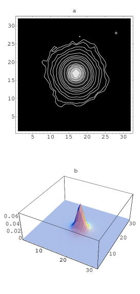
Figure 2: Normalized PSF of the A370 image.
a) Contours Plot. The contours represent successively 100, 80, 60, 40, 20, 10, 5, 3.5, 2.5, 1.5, 0.8, 0.5, 0.2, 0.1 $\%$ of the image maximum.
b) 3D Representation.

4 Deconvolution of the A370 CFHT image

4.1 Limitation of the standard Richardson-Lucy algorithm: ringing effects

We first deconvolve the A370 image with the classical Richardson-Lucy algorithm [Lucy (1974), Richardson (1972)] and the PSF previously estimated:

$$x^{(k+1)}=x^{(k)}.H^{T}\frac{y}{Hx^{(k)}}$$ (6)

where $x^{(k)}$ represents the reconstructed object at the iteration $k$, $y$ is the observation, $H$ is the PSF matrix and $H^{T}$ its transposed.

To stop the iterations of the algorithm we define an error criterion between the image reconstructed at iteration $k$ (denoted $x^{(k)}$) and a reference image. In this section we use the HST image (denoted $x^{HST}$) as the reference. We then minimize a criterion $R_{k}$ based upon a relative Euclidean distance between $x^{(k)}$ and $x^{HST}$:

$$R_{k}=\frac{\parallel x^{HST}-x^{(k)}\parallel}{\parallel x^{HST}\parallel}$$ (7)

where $\parallel.\parallel$ represents the Euclidean distance.
The objects in the field are rather different (giant arc, galaxies, stars…) and would not require exactly the same iteration number to be reconstructed at the best. The criterion $R_{k}$ must then be computed preferably over the area to be preferentially restored. We focus here on the region of the giant gravitational arc and thus minimize $R_{k}$ (see Figure 3) within the rectangular box indicated in Figure 1. The best reconstructed image obtained at iteration $k=50$ is represented in Figure 4.

Figure 3: Relative error curve $R_{k}$ between the CFHT reconstructed image and the HST one as a function of the iteration number for RL. The images used are those of the figure 1, the PSF is the one of figure 2 and the mask used correspond to the rectangular box ($20\times 28$ pixels).

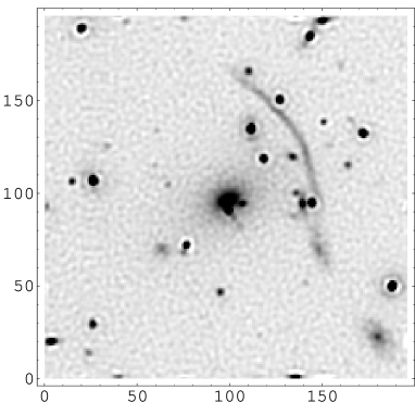
Figure 4: Abell 370 reconstructed image by RL at the 50th iteration. The image used is the one of figure 1 a), the PSF is the one of figure 2 and the mask used correspond to the rectangular box ($20\times 28$ pixels).

Its background shows a granular structure typically of the size of the PSF. An early ringing effect [Cao et al. (1999), Lucy 1994 a) , Lagendijk & Biemond (1991)] appears around the brightest point-like objects. It is both caused by the important background in the CFHT image and the discontinuities in the FT due to bright point-like objects [White (1993)]. These phenomena prevent any accurate measurement on the restored image and render necessary the use of a modified version of the algorithm to remove the oscillations. It is achieved by taking into account the background in the image and by introducing it as a lower bound constraint in the deconvolution algorithm itself. Hence, the reconstruction is not allowed to take values less than the background.

4.2 Amelioration: Lower Bound Constraint Algorithm (LBCA)

The LBCA is developed from a method proposed in [Lantéri et al. (2001)] and studied in detail in [Roche (2001), Lantéri et al. (2002)]. The method is based on the minimization of a convex function under lower bound constraint (denoted $m$). It consists in writing that at the optimum, the Kuhn-Tucker conditions [Kuhn & Tucker (1951)] are fulfilled. We then write the algorithm under a modified gradient form using the successive substitution method [Hildebrand (1974)]. After simple algebra, this leads in the non-relaxed case to the following multiplicative expression of the LBCA:

$$x_{i}^{(k+1)}=m_{i}+(x^{(k)}_{i}-m_{i})\left[H^{T}\frac{y}{(Hx^{(k)})}\right]_{i}$$ (8)

where $i$ is the current pixel in the image. A similar algorithm has been proposed by [Snyder et al. (1993)] and by [Nunez & Llacer (1993)] with however a slightly different formulation. A comparison between the two approaches is given in the Appendix. Note that when $m=0$ whatever the iteration, the RL algorithm is recovered.
The lower bound $m$ can be constant or variable over the image. The algorithm implementation is just as simple in both cases. The difficulty consists in obtaining an accurate background map specially in the region of bright structures. This estimation is out of the scope of this paper. We have then chosen to take for $m$ a constant value overall the image estimated as the mean background in the global normalized CFHT image.

We still stop the LBCA by minimizing the $R_{k}$ criterion (7). We evaluate $R_{k}$ within the rectangular box of Figure 1 as in the previous section. The corresponding $R_{k}$ curve is represented on Figure 5. The best restoration for this region of the giant arc is obtained for the iteration 269 (Figure 6). We see from Figure 5 that a range of about 50 iterations around this value would yield reconstructions of similar quality.

Figure 5: Relative error curve $R_{k}$ between the CFHT reconstructed image and the HST one as a function of the iteration number for LBA. The images used are those of the figure 1, the PSF is the one of figure 2 and the mask used correspond to the rectangular box ($20\times 28$ pixels).

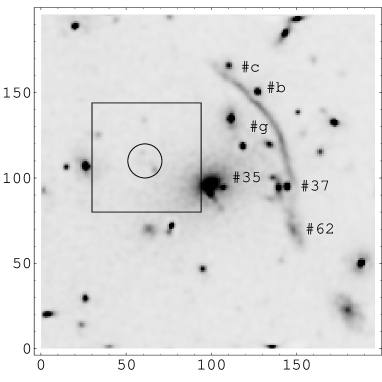
Figure 6: Best reconstructed image with LBCA using the HST reference image at the iteration 269.

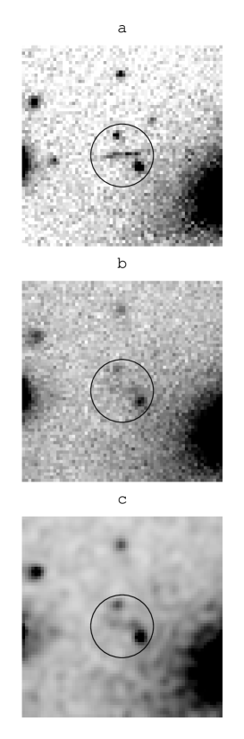
Figure 7: Zoom on the radial arc R. HST image (a), raw CFHT image (b) and deconvolved CFHT image (c).

The reconstructed image with the LBCA shows an important reduction of both granularity and ringing effects.
We use a criterion derived from $R_{k}$ to measure the amelioration brought by the deconvolution. We compute a quantity $D$ defined by:

$$D=100\times\frac{R_{y}-R_{opt}}{R_{y}}$$ (9)

where $R_{y}$ and $R_{opt}$ are defined as:

$$R_{y}=\frac{\parallel x^{HST}-y\parallel}{\parallel x^{HST}\parallel}\;\;\;,\;\;\;R_{opt}=\frac{\parallel x^{HST}-x^{(k_{opt})}\parallel}{\parallel x^{HST}\parallel}$$ (10)

$R_{y}$ and $R_{opt}$ measure the relative Euclidean distances between the HST reference $x^{HST}$ and the CFHT image before deconvolution $y$, and between $x^{HST}$ and the optimal restoration $x^{(k_{opt})}$. $D$ gives the averaged amelioration in percent with respect to the Euclidean measure. It raises up to 53$\%$ for the giant arc. We have also carried the minimization of $R_{k}$ for the full 196$\times$196 image and obtained a 47$\%$ amelioration with respect to the $D$ criterion. This means that the image obtained after deconvolution with the LBCA is closer to the HST image by roughly a factor 2 than the image before deconvolution. No significant amelioration is brought by the RL algorithm with this criterion.

This study shows a great amelioration carried out by the simple introduction of the lower bound constraint.
The deconvolution allows in particular to restore severals structures in the giant arc ($\#$b, $\#$c, $\#$g, $\#$37, $\#$62), and the breaking between $\#$37 and $\#$62. Moreover, the reconstructed image evidences a radial gravitational arc (circle in Figure 6 and 7.c). This arc is clearly visible in the HST image (Figure 7.a) but does not appear in the raw CFHT data (Figure 7.b).
Ringing residuals, while attenuated, are still present around high intensities objects. These drawbacks are due to an incorrect estimation of the background in these regions. The reconstruction can be improved by estimating a variable background.

We emphasize that the LBCA process takes the same computation time as the RL algorithm.

5 Wiener filtering for stopping iterations

We have used in the previous section a HST image to stop the iterations of the deconvolution. Usually, such a reference image is not available. Further, the objective is precisely to restore information from the sole ground-based observations without any external help. So it is necessary to develop a self-consistent method relying on the ground-based data only.
The technique we used is the one proposed by Lantéri et al. [Lantéri et al. (1999)]. It makes use of a comparison of the modulus of the Fourier transform of the deconvolved image at the iteration $k$ with the modulus of the Fourier transform given by a Wiener filtering. For clarity, let us briefly recall some well-known results on Wiener filtering. The Wiener filter $W(u,v)$ is a zero-phase filter that prevents the amplification of the noise if a raw inverse filter technique is used. Denoting $r$ the angular coordinates and $u$ and $v$ the 2D spatial frequencies, $\widehat{y}(u,v)$ and $\widehat{h}(u,v)$ the FT of the observation $y(r)$ and the PSF $h(r)$, the inverse Wiener filtered image transform $\widehat{x}_{w}(u,v)$ may be written as [Brault & White (1971)]:

$$\widehat{x}_{w}(u,v)=\frac{\widehat{y}(u,v)}{\widehat{h}(u,v)}W(u,v)$$ (11)

where $W(u,v)$ is defined as:

$$W(u,v)=\frac{P_{Hx}(u,v)}{P_{Hx}(u,v)+P_{n}(u,v)}$$ (12)

The quantities $P_{Hx}(u,v)$ and $P_{n}(u,v)$ are the power spectra of the noiseless image and of the noise itself respectively. Estimating these quantities is the main difficulty in the implementation of a Wiener filter. Only approximated expressions can be worked out. Assuming that the signal and noise are statistically independent, $P_{n}(u,v)$ can be taken as a constant. Its value may be estimated in the very high frequencies of $\widehat{y}(u,v)$, where no astronomical signal is expected. Estimating $P_{Hx}(u,v)$ is more difficult since it implies an a priori knowledge of the object FT. In the present work, we have assumed that $P_{Hx}(u,v)$ could be approximated by $P_{h}(u,v)$, the power spectrum of the telescope-atmosphere PSF. This tends to overestimate $W(u,v)$. So, after this procedure, equations 11 and 12 permit to have an estimate of $\widehat{x}_{w}(u,v)$. Following the work of Lantéri et al. [Lantéri et al. (1999)], we use only its modulus Abs$[\widehat{x}_{w}(u,v)]$ to define a stopping criterion for the LBC algorithm. At each iteration $k$, we compute the euclidean distance $E_{w}(k)$ of the form :

$$E_{w}(k)=\frac{\parallel\rm{Abs}[\widehat{x}^{(k)}(u,v)]-\rm{Abs}[\widehat{x}_{w}(u,v)]\parallel}{\parallel\rm{Abs}[\widehat{x}_{w}(u,v)]\parallel}$$ (13)

The raw application of this criterion fails to give a satisfactory iteration stop. A much better solution was found in using only in this comparison a range of intermediate frequencies. Indeed it was found necessary to suppress the very low frequencies that have a too important weight in the calculus. The comparison must also exclude the highest spatial frequencies that are suppressed by the Wiener filter used. The overall effect is to apply an annular mask in the frequencies plane.
Both Abs$[\widehat{x}^{(k)}(u,v)]$ and Abs$[\widehat{x}_{w}(u,v)]$ are normalized inside this mask for comparison. The distance $E_{w}(k)$ is represented as a function of the iteration number $k$ on Figure 8.

Figure 8: Relative error curve $E_{w}(k)$ between the modulus of the FT of the reconstructed image at iteration $k$ (Abs$[\widehat{x}^{(k)}(u,v)]$) and the FT of the Wiener reconstructed image (Abs$[\widehat{x}_{w}(u,v)]$).

The best reconstruction is obtained for the iteration k = 129 (Figure 9).

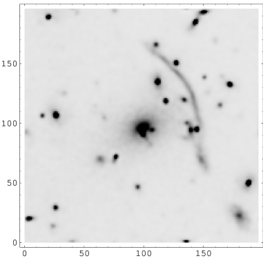
Figure 9: Best reconstructed image with LBCA using a criterion based on the Wiener filter at the 129th iteration.

The amelioration brought by the deconvolution estimated from the $D$ criterion (9) reaches 48$\%$. It is close to the 53$\%$ amelioration obtained in section 4.2 using the HST reference. It shows that independently of a reference HST image, a rather satisfying approximate solution may be found by using a stopping criterion based on the data themselves. This procedure can be fully and easily automated.

6 Conclusion

We have used a modified version of the RL algorithm, called LBCA, to deconvolve a CFHT image of Abell 370. The LBCA introduces a lower-bound constraint which prevents the reconstructed image to take values below this bound. It allows to reduce considerably the ringing effect that appears around bright objects when classical algorithm are used (in particular RL). In the present paper, the lower bound is taken equal to an estimation of the mean sky background over the whole CFHT 196$\times$196 image.
We have used at first an HST image of A370 as a reference to stop the iteration of the algorithm and to evaluate the amelioration brought by the deconvolution. An Euclidean distance criterion is then minimized between the reconstructed image at a given iteration and the HST reference to yield the best reconstruction. The LBCA reconstruction of A370 is twice as close to the HST image than the raw CFHT data, while no amelioration is brought by using the RL algorithm. Remarkably, our iterative process has permitted to detect blindly the radial arc evidenced earlier on HST image of A370 and to recover its morphological properties. This is an encouraging demonstration of its efficiency, and an interesting example of practical application. It also emphasizes the interest of the LBCA to restore images with a high background.
In a more general case where no HST image is available, the convergence and stopping rules of the algorithm must rely on the information contained in the data themselves. We have thus developed a technique using the Wiener filter. It proceeds from an estimation of the noise in the CFHT image and the evaluation of the Power spectrum of the PSF. This method is based on the minimization of an Euclidean distance between the FT modulus of the LBCA reconstruction and the reconstructed image by the inverse Wiener filter. The best reconstructed image is close to the former one obtained with the HST as a reference.

The present study evidences two important results. First, it allows to improve the quality of an image with a high background, using a new algorithm as simple and as fast as the RL one: the LBCA. Finally, the overall data processing involving the LBCA together with the Wiener filtering may be fully automated. Hence, it could be fruitfully used for the processing of huge amount of ground-based observations and particularly in the perspective of current or forthcoming wide field surveys.

Appendix A

We show in this appendix, the similarities between the algorithm used in the present paper and the algorithm previously proposed by [Snyder et al. (1993)] and by [Nunez & Llacer (1993)], to take into account the effect of the background.

In our algorithm written in the form 8:

$$x_{i}^{(k+1)}=m_{i}+(x^{(k)}_{i}-m_{i})\left[H^{T}\frac{y}{(Hx^{(k)})}\right]_{i}$$ (14)

$x$ is clearly the overall value of the solution, and we must have:

$$x_{i}\geq m_{i}\hskip 2.84544pt\forall i$$ (15)

Therefore, $x$ includes the background (the background $m$ is in the object space). The model used is $\tilde{y}=Hx$ and the actual data $y$ is Poisson with mean $Hx$. Now, introducing $u=x-m$ in this algorithm, we obtain immediately:

$$u_{i}^{(k+1)}=u^{(k)}_{i}\left[H^{T}\frac{y}{(H(u^{(k)}+m)}\right]_{i}$$ (16)

This the form previously proposed by [Snyder et al. (1993)] and by [Nunez & Llacer (1993)].
Here the model used is $\tilde{y}=H(u+m)$, $u$ is the part of the signal over the background $m$, and $u_{i}\geq 0$ $\forall i$. The background is again in the object space and the actual data $y$ is Poisson with mean $H(u+m)$.
Except these small conceptual differences, both algorithms are similar and leads to the same results, however another important point must be underlined. Because of the convolution, the mean $H(u+m)$ can also be written $Hu+m$ so the background $m$ appears in the data space). However it does not mean that we can subtract the background $m$ from the data $y$ for obtaining modified data $y^{\prime}=y-m$; indeed if $y$ is Poisson with mean $Hu+m$ , then $y^{\prime}$ is not Poisson of mean $Hu$ ($y^{\prime}$ might also be negative).
Then, whatever the form of the algorithm, the estimated background is used in the algorithm [Hanisch (1993)], but the data $y$ must left unchanged.

References

- Bertin & Arnouts (1996) Bertin, E. & Arnouts, S., 1996, A&AS, 317, 661.
- Bézecourt et al. (1999) Bézecourt, J., Kneib, J. P., Soucail, G. & Ebbels, T.M.D, 1999, A&AS, 347, 21.
- Boulade et al. (2000) Boulade, O., Charlot, X., Abbon, P., Aune, S., Borgeaud, P., Carton, P.-H., Carty, M., Desforge, D., Eppele, D., Gallais, P., Gosset, L., Granelli, R., Gros, M., de kat, J., Loiseau, D., Mellier, Y., Ritou, J.-L., Rousse, J.-Y., Starzinski, P., Vignal, N., Vigroux, L., 2000, SPIE 4008, 657.
- Brault & White (1971) Brault, J. W. & White, O. R., 1971, A& A, 13, 169.
- Cao et al. (1999) Cao, Y., Eggermont, P. P. B. & Terebey, S., 1999, IEEE. Trans. Image Processing, 8(2), 286.
- Hanisch (1993) Hanisch, B., 1993, Newsletter of STScI’s Image Restoration Project, 1, 70.
- Hildebrand (1974) Hildebrand F. B., 1974, Mac Graw Hill - N. Y.
- Kuhn & Tucker (1951) Kuhn, W. W. & Tucker, A. W., 1951, Proc. 2nd Berkeley Symp. on Mathematical Statistics and Probabilities, University of California Press, Berkeley, 481-491.
- Kneib et al. (1993) Kneib, J.-P., Mellier, Y., Fort, B., & Mathez, G., 1993, A&A 273, 367.
- Lagendijk & Biemond (1991) Lagendijk R.L. & Biemond J., 1991, Jluwer Academic, Publishers, London.
- Lantéri et al. (2002) Lantéri, H., Roche, M., Gaucherel, P. & Aime, C., 2002, Signal Processing, 82, 1481.
- Lantéri et al. (2001) Lantéri, H., Roche, M., Cuevas, O. & Aime, C., 2001, Signal Processing, 81(5), 945.
- Lantéri et al. (1999) Lantéri, H., Soummer, R., Aime, C., 1999, A & AS, 140, 235.
- Lucy (1974) Lucy, L.B., 1974, AJ, 79, 745.
- (15) Lucy, L.B., 1994,The restoration of HST images and spectra II. Space Telescope Institute, Hanisch R.J. and White R.L. eds, 79-85.
- Lynds & Petrosian (1986) Lynds, R. & Petrosian, V., 1986, BAAS, 18, 1014.
- Mellier et al. (1998) Mellier, Y., Soucail, G., Fort, B., & Mathez, G., 1998, A&A, 199, 13.
- Nunez & Llacer (1993) Nunez, J. & Llacer, J., 1993, PASP, 105, 1192.
- Roche (2001) Roche, M., 2001, Ph. D Thesis, University of Nice Sophia Antipolis.
- Richardson (1972) Richardson, W. H., 1972, Journal of Optical Society of America, 62(1), 55.
- Sarazin et al. (1982) Sarazin, C. L., Rood, H. J. and Struble, M. F., 1982, A & A, 108, L7.
- Sekko et al. (1999) Sekko, E., Thomas, G. and Boukrouche, A., 1999, Signal Processing, 72: 23-32.
- Smail et al. (1996) Smail, I., Dressler, A., Kneib, J. P. & al., 1996, ApJ, 469, 508.
- Snyder et al. (1993) Snyder, D. L., Hammoud, A. W. & White, R. L., 1993, JOSA A, 10, 1014.
- (25) Soucail, G., Fort, B., Mellier, Y. & Picat, J.P., 1987 a), A&A, 172, L14-L16.
- (26) Soucail, G., Mellier, Y., Fort, B., Hammer, F. & Mathez, G., 1987 b), A&A, 184, L7-L9.
- Soucail et al. (1988) Soucail, G., Mellier, Y., Fort, B., Mathez, G., & Cailloux, M., 1988, A&A, 191, L19.
- Valentijn et al. (2001) Valentijn, E. A., Deul, E., Kuijken, K., 2001, in The New Era of Wide Field Astronomy, ASP Conf. Ser. Vol. 232. R. Clowes, Adamson, A. and Bromage, G. Eds.
- White (1993) White, R. L., Newsletter of STScI’s image restoration project, Summer 1993, 1, 11.
- Wiener (1949) Wiener, N., 1949, Wiley, New York.