Exploring the sub-eV neutrino mass range with supernova neutrinos

Abstract

A new method to study the effects of neutrino masses on a supernova neutrino signal is proposed. The method relies exclusively on the analysis of the full statistics of neutrino events, it is independent of astrophysical assumptions, and does not require the observation of any additional phenomenon to trace possible delays in the neutrino arrival times. The sensitivity of the method to the sub-eV neutrino mass range, defined as the capability of disentangling at 95% c.l. the case $m_{\nu}=1\,$eV from $m_{\nu}=0$, is tested by analyzing a set of synthetic neutrino samples modeled according to the signal that could be detected at SuperKamiokande. For a supernova at the Galactic center success is achieved in more than 50% of the cases. It is argued that a future Galactic supernova yielding several thousands of inverse $\beta$ decays might provide enough information to explore a neutrino mass range somewhat below $1\,$eV.

During the past few years, the large amount of data collected by solar solar and atmospheric atmospheric neutrino experiments provided strong evidences for non vanishing neutrino masses. The recent KamLAND result kamland on the depletion of the neutrino flux from nuclear power plants in Japan, gave a final confirmation of this picture. Since in the Standard Model (SM) of particle physics all neutrino species are massless, this constitutes the first direct evidence for new physics, and provides important informations for developing theories beyond the SM. However, to date all the evidences for neutrino masses come from oscillation experiments, that are only sensitive to mass square differences and cannot give any informations on single mass values. The importance of measuring the absolute value of neutrino masses cannot be understated. It is presently being addressed by means of a remarkably large number of different approaches, ranging from laboratory experiments to a plethora of methods that relay on cosmological considerations. Recent reviews can be found in absolutenumass . From the study of the end-point of the electron spectrum in tritium $\beta$-decay, laboratory experiments have been able to set the limit $m_{\nu_{e}}<2.2\,$eV tritiumlimit . This is already close to the sensitivity limit of on-going experiments. If neutrinos are Majorana particles, the non observation of neutrinoless double $\beta$ decay can constrain a particular combination of the three neutrino masses. Interpretation of these experimental results is difficult due to large theoretical uncertainties related to nuclear matrix elements calculations. This is reflected in a model dependent limit $m_{\nu}^{eff}<0.35-1.24\,$eV absolutenumass ; doublebeta . A tight bound $\sum_{i}m_{\nu_{i}}<0.7\,$eV was recently set by the WMAP Collaboration WMAP by combining measurements of cosmic microwave background anisotropies with data from bright galaxies redshift surveys Colless:2001gk and other cosmological data. However, this limit becomes much looser if the set of assumptions on which it relies is relaxed (see Hannestad for discussions of this point). Therefore it is quite important to keep looking for alternative ways to measure the neutrino masses. Model independent limits can be more reliably established by combining complementary experimental informations and, needless to say, it would be of utmost importance if the mass values could be measured by means of more than one independent method.

Already long time ago it was realized that Supernova (SN) neutrinos can provide valuable informations on the neutrino masses Zatsepin:1968 . The basic idea relies on the time-of-flight delay $\Delta t$ that a neutrino of mass $m_{\nu}$ and energy $E_{\nu}$ traveling a distance $L$ would suffer with respect to a massless particle:

$$\frac{\Delta t}{L}=\frac{1}{v}-1\approx\left(\frac{5.1\,\rm ms}{10\,\rm kpc}\right)\!\left(\frac{10\,\rm MeV}{E_{\nu}}\right)^{2}\!\!\!\left(\frac{m_{\nu}}{1\,\rm eV}\right)^{2}\,,$$ (1)

where for ultra-relativistic neutrinos we have used $1/v=E_{\nu}/p_{\nu}\simeq 1+m^{2}_{\nu}/2E_{\nu}^{2}$. The dispersion in the arrival time of about twenty electron anti-neutrinos from supernova SN1987A was used in the past to set the model independent limit $m_{\bar{\nu}_{e}}<30\,$eV Schramm:1987ra . This limit can become significantly tighter under some specific assumptions. For example a recent detailed reanalysis obtained, within the SN delayed explosion scenario, the limit $m_{\bar{\nu}_{e}}<5.7\,$eV Loredo:2001rx .

Since SN1987A, several efforts have been carried out to improve the sensitivity of the method, while awaiting for the next explosion within our Galaxy. Often, these approaches rely on “timing” events related to the collapse of the star core, that are used as benchmarks for measuring the neutrino delays. The emission of gravitational waves gravit1 ; gravit2 , the $\nu_{e}$ neutronization burst gravit2 , the initial steep raise of the neutrino luminosity steep , and the abrupt interruption of the neutrino signal due to a further collapse into a black hole blackhole have been used to this aim. However, there are some drawbacks to these methods: firstly only neutrinos with arrival time close to the benchmarks are used, and they represent only a small fraction of the total; secondly the observation of the benchmark events is not always certain, and in any case some model dependence on the details of the SN explosion is generally introduced.

The method we want to propose is free from these drawbacks: it relies only on the measurement of the neutrinos energies and arrival times, and it uses the full statistics of the detected signal, thus allowing to extract the maximum of information. It is also remarkably independent of particular astrophysical assumptions, since no use is made of benchmarks events. The basic idea is the following: in the idealized case of vanishing experimental errors in the determination of the neutrino energies and arrival times, and assuming an arbitrarily large statistics and a perfectly black-body neutrino spectrum, one could use the events with energy above some suitable value $E^{*}$ (to suppress the mass effects) to reconstruct very precisely the evolution in time of the neutrino flux and spectrum. Once the time dependence of the full signal is pinned down, the only parameter left to reconcile the time distribution of the low energy neutrinos with the high energy part of the signal would be the neutrino mass, that could then be nailed to its true value. Of course, none of the previous conditions is actually fulfilled. In water Čerenkov detectors as SuperKamiokande (SK) the uncertainty on relative timings is negligible; however, the errors in the energy measurements are important and must be properly taken in to account. The statistics is large but finite, and this not only represents a source of statistical uncertainty, but also implies an upper limit on the useful values of $E^{*}$. Finally, the SN neutrino spectrum is not perfectly thermal neutrino-spectrum . Nevertheless, a good sensitivity to the mass survives and, as we will show, it will be possible to disentangle with a good confidence the two cases $m_{\nu}=0$ and 1 eV.

To test quantitatively the idea outlined above we proceed in two steps:

i) First we generate a set of synthetic neutrino signals, according to some suitable SN model. Neutrinos are then propagated from the SN to the detector assuming two different SN-Earth distances (10 and 20 kpc) and two different mass values $m_{\nu}=0\,$ and $1\,$eV. Finally, two different energy thresholds (5 and 10 MeV) are used for the detection. The result consists of several neutrino samples, that hopefully would not differ too much from a real SN signal.

ii) The signals are then analyzed with the main goal of disentangling with sufficient confidence the two cases $m_{\nu}=0\,$ and $1\,$eV. Only the SN-Earth distance is assumed to be known (this information could be obtained directly from optical observations or, with an uncertainty of the order of 25%, from a comparison of the measured total energy with a theoretical estimation of the binding energy released located ). Other quantities, like the spectral functions and the details of the time evolution of the neutrino flux, are inferred directly from the data.

Generation of the neutrino samples. The time evolution of the neutrino luminosity and average energy can be obtained from the results of SN explosions simulations burrows ; woosley ; totani ; lieben . In the present analysis we use the results of Woosley et al. woosley . This model is characterized by a rather hard neutrino spectrum ($\langle E_{\bar{\nu}_{e}}\rangle\ \hbox to0.0pt{\raise 3.0pt\hbox{$>$}\hss}{\lower 3.0pt\hbox{$\sim$}}\ 20\,$MeV) that results in a large number of detected events (8,800 in SK). Still this is a conservative choice, since it also implies a depletion in the number of low energy neutrinos with a corresponding loss of informations on the neutrino mass. Inside the protoneutron star neutrinos are in thermal equilibrium, and therefore it is reasonable to assume that the gross features of their energy spectrum after emission can still be described by a Fermi-Dirac distribution:

$$\widehat{S}\left(E_{\nu};\hat{T}(t),\hat{\eta}\right)=\frac{E_{\nu}^{2}/\hat{T}^{3}(t)}{F_{2}(0,\hat{\eta})\,\left(1+e^{E_{\nu}/\hat{T}(t)-\hat{\eta}(t)}\right)},$$ (2)

where $F_{2}(0,\hat{\eta})$ is defined in (4) and a ‘pinching’ factor $\hat{\eta}(t)$ has been introduced to simulate spectral distortions neutrino-spectrum . From now on, quantities with a hat ($\hat{\eta}$, $\hat{T}$, …) represent inputs to the Monte Carlo (MC), while quantities without a hat will refer to results of data fitting. We define the Fermi functions and generalized Fermi integrals as:

$$f_{n}(x,\eta) = \frac{x^{n}}{1+e^{x-\eta}}$$ (3)

$$F_{n}(y,\eta) = \int^{\infty}_{y}{f_{n}(x,\eta)}\,dx\,.$$ (4)

Using the time evolution of the average neutrino energy $\overline{E_{\nu}}(t)$ as given in fig. 3 of ref. woosley and taking for simplicity $\hat{\eta}=3$ neutrino-spectrum constant, we compute the effective temperature that, together with $\hat{\eta}$, determines the neutrino spectrum at the source:

$$\hat{T}(t)=k_{3}\>\overline{E_{\nu}}(t)\,,$$ (5)

where $k_{3}\equiv F_{2}(0,3)/F_{3}(0,3)\approx 4$. Given that the average energy is only mildly dependent on time woosley , we model the evolution of the neutrino flux $\widehat{\Phi}(t)$ simply by taking it proportional to the luminosity as given in fig. 2 of ref. woosley .

In the SK detector, $\bar{\nu}_{e}$’s are detected through the inverse $\beta$ decay reaction $\bar{\nu}_{e}\,p\to e^{+}\,n$ that has the energy threshold $E_{\rm react}=m_{e}+\Delta m_{np}\simeq 1.8\,$MeV, where $m_{e}$ is the electron mass and $\Delta m_{np}\simeq 1.3\,$MeV is the neutron to proton mass difference. The effect of the detection cross section $\sigma(E_{\nu})$ Strumia:2003zx is taken into account from the beginning by using the function $\widehat{S}\big{(}E_{\nu};\hat{T}(t),\hat{\eta}\big{)}\times\widehat{\Phi}(t)\times\sigma(E_{\nu})$ in the MC generator. Each SN neutrino is labeled by its emission time $t_{\nu}$ and by its energy $E_{\nu}$. The corresponding detected positron is also identified by an energy/time pair of values $(E^{e},t^{e})$. We generate $E^{e}$ according to a Gaussian distribution with central value $E^{e}=E_{\nu}-\Delta m_{np}$ and variance $\sigma=0.15\,\sqrt{10\,{\rm MeV}/E^{e}}\,$ that corresponds to the SK energy resolution SKresolution . Since the time resolution of the SK detector is very precise, no error is assigned to $t^{e}$. For massive neutrinos, we redefine $t^{e}=t_{\nu}+\Delta t_{\nu}$ by including the appropriate delay $\Delta t_{\nu}=L\,m^{2}_{\nu}/2\,E^{2}_{\nu}$. A fixed number of 8,800 energy/time pairs $(E^{e}_{i},t^{e}_{i})$ is generated in each run. This corresponds to the expected number of $\bar{\nu}_{e}$ interactions within the SK fiducial volume for the spectrum of the model in woosley and a SN at $10\,$kpc. For $L=20\,$kpc this number is resampled down by a factor of four. Next, positrons with energies below the detection threshold ($E_{\rm tr}=5\,$ or $10\,$Mev) are discarded, and as a last step the origin of the time axis is set in coincidence with the first positron detected ($t^{e}_{1}=0$) and each $t^{e}_{i}$ is accordingly redefined. For each set of values ($E_{\rm tr}\,,L\,,m_{\nu}$) forty different samples are generated in this way.

Analysis of the neutrino signal.  We analyze the neutrino signals by means of the likelihood function

$${\cal L}=S\big{(}\epsilon;T(t),\eta(t)\big{)}\times\Phi(t+\delta t;b,d,f)\times\sigma(\epsilon)\,.$$ (6)

The energy $\epsilon=E^{e}+\Delta m_{np}$ of each neutrino is inferred from the positron energy. The spectral function $S$ is assumed of the form (2) with a time dependent effective temperature $T(t)$ and pinching factor $\eta(t)$ fitted from the data. $\Phi(t+\delta t;b,d,f)$ describes the time evolution of the neutrino flux, and the four parameters $\delta t\,,b\,,d$ and $f$ account for its location on the time axis and detailed shape. Finally, $\sigma(\epsilon)$ is the neutrino cross section.

Figure 1: Comparison of the Monte Carlo spectral temperature $\hat{T}(t)$ and pinching parameter $\hat{\eta}$ (thick lines), with $T(t)$ and $\eta(t)$ fitted for 40 samples ($L=10\,$kpc, $m_{\nu}=0\,$).

The spectral functions. The two spectral functions $T(t)$ and $\eta(t)$ are determined by fitting the first and second momentum of the energy distribution to the mean energy $\overline{E_{\nu}}$ and mean squared energy $\overline{E_{\nu}^{2}}$ of the incoming neutrino flux (prior to detection). Given a set of $n$ neutrinos with measured energies $(\epsilon_{1},\epsilon_{2},\dots.\epsilon_{n})$, and assuming for the cross section the approximate form $\sigma(\epsilon)\propto{\epsilon}^{2}$, we have:

$$\overline{E_{\nu}}\approx\frac{\sum_{i}\epsilon_{i}^{-1}}{\sum_{i}\epsilon_{i}^{-2}};\qquad\quad\overline{E^{2}_{\nu}}\approx\frac{n}{\sum_{i}\epsilon_{i}^{-2}}.$$ (7)

From (1) we see that the typical neutrino delays are at most of the order of few milliseconds. This is much shorter than the time scale over which sizable variations of the spectral functions are likely to occur burrows ; woosley ; totani ; lieben . Therefore, by binning over sufficiently large time windows we can ensure that the determination of $T$ and $\eta$ for each bin will not be affected by the delays. We use a set of 20 windows of size increasing from 50 ms to 2 s, distributed over a signal duration 20 s. After this time the neutrino flux is assumed to be too low to provide additional informations. To reduce further the possible effects of mass induced time delays, only neutrinos with energy larger than $E^{*}=15\,$MeV are used. For each time window [$t_{a}$, $t_{a+1}$] we perform a least square fit to the following quantities:

$$\overline{E_{\nu}}(T,\eta) = \frac{F_{3}(y,\eta)}{F_{2}(y,\eta)}\,T\,,$$ (8)

$$\frac{\overline{E_{\nu}^{2}}(T,\eta)}{\left[\overline{E_{\nu}}(T,\eta)\right]^{2}} = \frac{F_{2}(y,\eta)\>F_{4}(y,\eta)}{F^{2}_{3}(y,\eta)}\,,$$ (9)

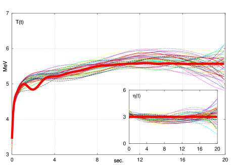
where the functions $F_{n}(y,\eta)$ defined in (4), depend on the temperature through $y={E^{*}/T}$. This yields the ‘best’ values $T(\bar{t}_{a})$ and $\eta(\bar{t}_{a})$ at $\bar{t}_{a}=(t_{a}+t_{a+1})/2$. Finally, in order to obtain two smooth continuous functions, the points $T(\bar{t}_{a})$ and $\eta(\bar{t}_{a})$ are interpolated with two half integer power polynomials $P_{T,\eta}\sim\sum_{l}c_{l}t^{l/2}$ with $l=0,1,2,\dots 10$ for $T$ and $l=0,1,3,5$ for $\eta$. In fig. 1 the functions $\hat{T}(t)$ and $\hat{\eta}=3$ used in the MC (thick lines) are compared with forty fits to neutrino samples generated with $m_{\nu}=0$ and $L=10\,$kpc. These results remain unchanged for $m_{\nu}=1\,$eV, while for $L=20\,$kpc, due to the reduced statistics, the fits show a somewhat wider dispersion.

The neutrino flux. Even if the details of the neutrino flux evolution with time are not known, its gross features can be predicted on rather solid theoretical grounds. It is expected that a sharp exponential rise, with a time scale of tenths of milliseconds, is followed by a power law decay, with a time scale of several seconds. We model this behavior by means of a parametric analytical function in which, roughly speaking, two parameters describe the rising and decaying rates, and a third one accounts for the transition point:

$$\Phi(t;b,d,f)\sim\frac{e^{-ft^{-m}}}{(1+b\,t^{n})^{d}}\to\left\{\begin{array}[]{ll}e^{-ft^{-m}}&(t\to 0)\\ t^{-nd}&(t\to\infty)\,.\end{array}\right.\quad$$ (12)

This function can reproduce reasonably well the results of different models woosley ; totani ; burrows ; lieben . The two exponents $m$ and $n$ are fixed to suitable integer values by means of a preliminary rough fitting procedure to the data, and then are held constant throughout the analysis of all the samples. For the model in woosley we use $n=8$ and $m=2$. Finally, since the origin of times was arbitrarily set in coincidence with the detection of the first neutrino while $\Phi$ vanishes at $t=0$, a fourth parameter $\delta t$ is required to let $\Phi(t+\delta t)$ freely shift along the time axis.

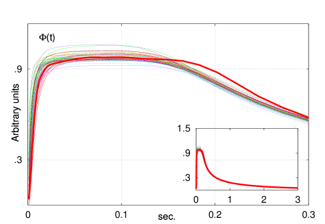
The likelihood analysis. The minimization of the negative log-likelihood is carried out by means of the package MINUIT minuit . To avoid double minimums, we minimize with respect to the square of the neutrino mass. Given a value of $m^{2}_{\nu}$ the time delay of each neutrino is computed according to its energy $\epsilon_{i}$, and subtracted from its arrival time $t_{i}$. The log-likelihood for the new array of times is then evaluated, and minimized with respect to the other parameters $b\,,d\,,f$ and $\delta t$. This proceeds until the absolute minimum is found in the full five dimensional parameter space. There is a subtlety related to the cases when, especially for large test masses, a neutrino is migrated to an early time where $\Phi=0$. The problem is not just a numerical one of logarithm overflow. Due to the uncertainty in the energy measurement, the firsts neutrinos detected can end up in such a position without necessarily implying that the corresponding distribution has vanishing probability. To account for this, for the relevant neutrinos the energy uncertainty is converted into an uncertainty in the new time position, and the corresponding contribution to the likelihood is evaluated by convolving ${\cal L}(t)$ in (12) with a Gaussian of the appropriated width. In fig. 2 the results of the fitted fluxes for 40 samples with $L=10\,$kpc, $E_{\rm tr}=5\,$MeV and $m_{\nu}=0\,$eV are compared with the function $\widehat{\Phi}(t)$ used in the MC generator (thick line).

Figure 2: Comparison between the Monte Carlo flux function $\widehat{\Phi}(t)$ (thick line), and the result of the likelihood analysis for 40 samples ($L=10\,$kpc, $E_{tr}=5\,$MeV, $m_{\nu}=0$).

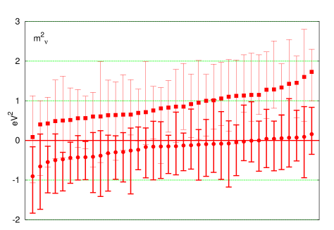
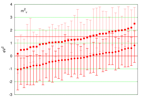
Results. Our results are summarized in fig. 3 and in table 1. Fig. 3 depicts the results of the mass fits for two sets of 40 samples with $E_{\rm tr}=5\,$MeV, $L=10\,$kpc, $\hat{m}_{\nu}=0$ (circles) and $\hat{m}_{\nu}=1\,$eV (squares). The data points have been ordered with increasing value of the best fit mass to put in evidence the difference between the two cases. Error bars correspond to 95% c.l., where the lower (upper) limit is computed by integrating the likelihood from $m^{2}_{\nu}=\infty$ ($-\infty$) until reaching the 95% of the area, while minimizing with respect to the other parameters. We have checked that the limits do not change much if the integration is restricted to the physical region $m_{\nu}^{2}>0$.

Table 1 summarizes some results of the mass fitting. For each set of parameters ($E_{\rm tr},\,L,\,\hat{m}_{\nu}$) we have analyzed 40 samples. The first raw gives the percentage of times in which the 95% c.l. lower limit $m^{l}_{\nu}$ is larger than the input mass $\hat{m}_{\nu}$. The second raw refers to the cases when the upper limit $m^{u}_{\nu}$ is smaller than $\hat{m}_{\nu}$. Number in parentheses correspond to $L=20\,$kpc. These figures characterize the percentage of ‘failures’ of the method, that therefore appears to be reliable in about 90%-95% of the cases. The third row gives the percentage of times when $m_{\nu}=0\,$ is excluded at 95% c.l. when the signal is generated with $\hat{m}_{\nu}=1\,$eV. This characterizes the power of the method for excluding a massless neutrino. We see that in the most favorable case ($E_{\rm tr}=5\,$MeV, $L=10\,$kpc) the method is successful in more than 50% of the cases. The following three raws give the average over the 40 samples of the mass square best fit and of the 95% c.l. lower and upper limits (only for $L=10\,$kpc). These last figures are just intended to give an idea of the quality of the fits (they would be fully meaningful only if 40 SN could be observed).

Figure 3: Fitted values of the mass and 95% c.l. error bars for two sets of 40 analysis with $L=10\,$kpc and $E_{tr}=5\,$MeV, for $\hat{m}_{\nu}=0$ (circles) and $\hat{m}_{\nu}=1\,$eV (squares).

$E_{{\rm tr}}$	5 MeV		10 MeV
$\hat{m}_{\nu}$ (eV)	0	1	0	1
$m_{\nu}^{l}>\hat{m}_{\nu}\,$(%)	5 (11)	4  (5)	5 (10)	11 (5)
$m_{\nu}^{u}<\hat{m}_{\nu}\,$(%)	9 (6)	2  (5)	12 (6)	10 (7)
$m_{\nu}^{l}>0\>$   (%)	–	55 (40)	–	28 (23)
$\left<m_{\nu}^{2}\right>$	–$0.1\pm 0.4$	$1.0\pm 0.5$	–$0.2\pm 0.8$	$\ 0.8\pm 1.0$
$\left<(m_{\nu}^{l})^{2}\right>$	–$0.8\pm 0.4$	$0.1\pm 0.6$	–$1.6\pm 1.0$	–$0.8\pm 1.2$
$\left<(m_{\nu}^{u})^{2}\right>$	$\ 0.6\pm 0.5$	$1.8\pm 0.5$	$\ 1.1\pm 1.0$	$\ 2.2\pm 1.1$

Table 1: Results of the analysis for the two neutrino masses $\hat{m}_{\nu}=0\,$ and $1\,$eV, two energy thresholds of $5$ and $10\,$MeV and for two SN distances of $10\,$kpc and, in parenthesis, $20\,$kpc. The first (second) row give the percentage of times in which the 95% c.l. lower (upper) limit $m_{\nu}^{l}$ ($m_{\nu}^{u}$) is larger (smaller) than $\hat{m}_{\nu}$. The third row lists how many times $m_{\nu}=0$ can be excluded (95% c.l.) when $\hat{m}_{\nu}=1\,$eV. The following three rows give, for $L=10\,$kpc, the mass square best fit and the 95% lower and upper limits averaged over 40 samples.

From the results in the table it is apparent that low energy neutrinos are crucial for the sensitivity of the method, and therefore a low detection threshold is very important. With $E_{\rm tr}=5\,$MeV the massless case is excluded in about 50% of the cases, while this drops to 25% when $E_{\rm tr}=10\,$MeV. Also, with the higher energy treshold the fluctuations of the results over the 40 runs is doubled (last three rows). Unfortunately, there could be a dangerous background in the energy range between 5 and 10 MeV, represented by photons originating from neutral current reactions off ¹⁶O mainly produced by the more energetic $\mu$ and $\tau$ neutrinos oxygen . Softer neutrino spectra, like for example the ones predicted by the model of Totani et al. totani , would have the double benefit of drastically reducing this background, while at the same time raising the number of $\bar{\nu}_{e}$ emitted in the 5-10 MeV energy range from about 7% of the present analysis to about 20%. In this case a better sensitivity to the mass could be expected. We should also mention that very recently it has been suggested that water Čerencov detectors could be modified to allow tagging of the inverse $\beta$ decay neutrons Beacom:2003nk . This would eliminate the background from neutral current reactions and allow for lower thresholds.

Numerical spectrum and neutrino oscillations. The previous results have been derived relying on two main simplifying approximations for the neutrinos energy spectrum: 1) the neutrino energies have been generated assuming the ‘pinched’ Fermi-Dirac spectrum given in eq. (2) and fitted, as was described above, with a similar two-parameters energy distribution; 2) no effects of the neutrino oscillations were included in the analysis. In order to evaluate to what extent the sensitivity of the method could be affected by these approximations, we have run a set of simulations in which the neutrino energies were generated according to the shapes of the numerical spectra given by Janka and Hillebrandt in neutrino-spectrum . A time dependent energy rescaling of the spectral shapes was introduced to reproduce properly the time evolution of the mean energies as given in woosley . We stress that since a two parameters Fermi-Dirac distribution fits rather accurately the spectra obtained from the numerical simulations, dropping our first simplification does not affect sensibly the numerical results.

Neutrino oscillations can produce a composite spectrum corresponding to an admixture of the original $\bar{\nu}_{e}$ spectrum with a harder component due to $\bar{\nu}_{x}$ ($x=\mu,\tau$) Lunardini:2003eh . Clearly, the resulting spectral distortions will depend in first place on the size of the $\bar{\nu}_{e}-\bar{\nu}_{x}$ spectral differences. While it is often stated that these differences could be quite sizable, and could yield up to a factor of two hierarchy between the $\bar{\nu}_{x}$ and $\bar{\nu}_{e}$ average energies burrows ; woosley ; totani ; lieben , recent and more complete analysis of SN neutrino spectra formation KeilRaffeltJanka indicate that this is not the case: the inclusion of important interaction rates that were neglected in previous works yields spectral differences that are only of the order of 10% KeilRaffeltJanka . At this level, identifying the two components of a mixed spectrum would be a difficult task, and could represent a real challenge for the study of SN neutrino oscillations in the $\bar{\nu}_{e}-\bar{\nu}_{x}$ channel. However, for what concerns our analysis, this ensures that the results discussed above are not affected much by neutrino oscillations. To keep on the safe side, we have tested the sensitivity of our method to oscillation effects by running a set of simulations using the results of Woosley et al. woosley for which, as a consequence of negelcting important neutrino reactions KeilRaffeltJanka , the spectral differences are extreme ($\overline{E}_{\bar{\nu}_{x}}\approx 2\,\overline{E}_{\bar{\nu}_{e}}$). As we will show, even in this (probably unrealistic) case, we find that the loss in sensitivity to the neutrino mass is small. We can conclude that the effects of neutrino oscillations do not endanger the applicability of our method and neither its overall sensitivity to the neutrino mass.

As is discussed in Lunardini:2003eh , depending on the type of the neutrino mass hierarchy (normal or inverted) and on the size of $\sin^{2}\theta_{13}$ (large $\ \hbox to0.0pt{\raise 3.0pt\hbox{$>$}\hss}{\lower 3.0pt\hbox{$\sim$}}\ 10^{-4}$ or very small $\ \hbox to0.0pt{\raise 3.0pt\hbox{$<$}\hss}{\lower 3.0pt\hbox{$\sim$}}\ 10^{-6}$), neutrino oscillations could i) harden the $\bar{\nu}_{e}$ spectrum through a complete spectral swap with $\bar{\nu}_{\mu}$ (inverted hierarchy, large $\theta_{13}$) ii) mix the $\bar{\nu}_{e}$ spectrum with a fraction of about $\sin^{2}\theta_{12}\sim 1/4$ of harder neutrinos (in the other cases). (The region $\sin^{2}\theta_{13}\sim 10^{-6}-10^{-4}$ would produce spectra with an intermediate amount of mixing.) The first case can be studied without modifications in our procedure. Clearly, a different spectrum would imply somewhat different numerical results; however, this is analogous to the unavoidable uncertainty related to the choice of the particular SN model since, for example, the $\bar{\nu}_{e}$ mean energies that have been used in the present analysis woosley are quite close to the $\bar{\nu}_{\mu}$ mean energies of the model of Totani et al. totani . The second case is more interesting since, for large spectral differences, fitting a composite spectrum with just one effective spectral temperature and one pinching parameter could degrade somewhat the sensitivity.

Figure 4: Comparison between the $\bar{\nu}_{e}$ (upper thick line) and $\bar{\nu}_{\mu}$ (lower thick line) fluxes used in the Monte Carlo, the resulting $\bar{\nu}_{e}$ flux at the detection point (middle thick line), and the maximum likelihood fits for 40 neutrino samples with a mixed composite spectrum.

Figure 5: Comparison between the $\bar{\nu}_{e}$ (lower thick line) and $\bar{\nu}_{\mu}$ (upper thick line) mean energies of the numerical spectra used in the Monte Carlo, the mean energy of the mixed composite spectrum (middle thick line), and the fitted values of $\overline{E}_{\bar{\nu}_{e}}(t)$ for 40 neutrino samples.

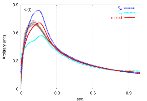
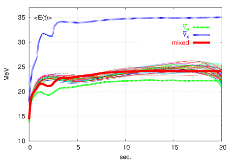
We have carried out an analysis of forty neutrino samples with a mixed composite spectrum as would result from a normal mass hierarchy, $\sin^{2}\theta_{12}\approx 1/4$ and large $\theta_{13}$. The original $\bar{\nu}_{e}$ and $\bar{\nu}_{x}$ fluxes taken from woosley are depicted in fig. 4 and compared with the composite $\bar{\nu}_{e}$ flux at the detection point, as well as with our maximum likelihood fits. The relative normalization of the fluxes was computed assuming flavor equipartition of the integrated luminosities and the time dependent average energies given in woosley . A similar comparison between the mean energies of the two spectral components, the average energy of the mixed spectrum and the average energies obtained from Fermi-Dirac distributions with fitted spectral parameters $\hat{T}(t)$ and $\hat{\eta}(t)$ is depicted in fig. 5.

For the mass fits we have taken $E_{\rm tr}=5\,$MeV and $L=10\,$kpc. Since we are essentially interested in the loss of sensitivity to the neutrino mass with respect to the non-oscillation case, we have been searching for a mass value that can reproduce results similar to those of the band plot in fig. 3 (namely, for a signal generated with $\hat{m}_{\nu}\neq 0$ we require the massless case to be excluded at 95% c.l. in at least 50% of the runs). As is shown in fig. 6 our requirement is fullfilled for $\hat{m}_{\nu}=1.2\,$eV, to be compared with $\hat{m}_{\nu}=1.0\,$eV for the non-oscillation case. We conclude that even in the unrealistic case of extremely large spectral differences between the components of a mixed spectrum, fitting the data with a single two parameters Fermi-Dirac distribution does not degrade much the numerical results for the mass estimate. Given that the most recent results suggest that the $\bar{\nu}_{e}$ and $\bar{\nu}_{\mu}$ spectra are in fact not very different KeilRaffeltJanka , the use of more complicated bimodal energy distributions to improve the mass fits is probably not justified.

Figure 6: Fitted values of the mass and 95% c.l. error bars for a set of 40 neutrino samples with mixed composite spectra ($L=10\,$kpc, $E_{tr}=5\,$MeV, $\hat{m}_{\nu}=0$ (circles), $\hat{m}_{\nu}=1.2\,$eV (squares)).

Before concluding, a few remarks are in order. In this work we have not carried out any deep study aimed to optimize the single fits to each different neutrino sample (windows size, interpolating functions $P_{T,\eta}$, specific flux function parameters). A large number of different sets of data have been analized through the very same procedure, in order to collect enough informations about the sensitivity of the method in a reasonable amount of time. It is clear to us that optimizing the overall procedure in order to analze a specific sample (as would certainly be the case with a signal from a real SN) can improve the sensitivity and shrink somewhat the uncertainties on $m^{2}_{\nu}\,$.

Besides the effects of neutrino oscillations that were briefly analyzed in the last paragraph, a few other issues could deserve further investigation. For example, assuming that the SK signal could be combined with negligible uncertainty on the absolute timing with the signal detected at KamLAND, the much better energy resolution and the lower threshold of this last detector could enhance the sensitivity to the neutrino mass. It also remains to see what sensitivity could be achieved with a statistics one order of magnitude larger, as would be available with the megaton neutrino detectors presently under study HyperK ; UNO ; TITAND .

Acknowledgments.

We acknowledge conversations with H.-T. Janka, G. Raffelt and in particular with A. Yu. Smirnov. J.I.Z. acknowledges hospitality from the Abdus Salam ICTP in Trieste (Italy) during the final stage of this research, and Colciencias for a scholarship for Doctoral Sudies. This work was supported in part by Colciencias in Colombia under contract 1115-05-13809.

References

- (1) S. Fukuda et al. Phys. Rev. Lett. 86, 5651 (2001); Q. Ahmad et al. Phys. Rev. Lett. 87, 071301 (2001).
- (2) Y. Fukuda et al. Phys. Rev. Lett. 81 1562 (1998); ibid. 82, 2644 (1999); M. Ambrosio et al. Phys. Lett. B434, 451 (1998); ibid. B478, 5 (2000).
- (3) K. Eguchi et al. Phys. Rev. Lett. 90, 021802 (2003).
- (4) H. Pas and T. J. Weiler, Phys. Rev. D 63, 113015 (2001); S. Bilenky et al., Phys. Rept. 379, 69 (2003);
- (5) J. Bonn et al., Prog. Part. Nucl. Phys. 48, 133 (2002); V. M. Lobashev et al., Nucl. Phys. Proc. Suppl. 91, 280 (2001).
- (6) H.V. Klapdor-Kleingrothaus et al., Eur. Phys. J. A12, 147 (2001); C.E. Aalseth et al., Phys. Rev. D65, 092007 (2002).
- (7) D. N. Spergel et al., Astrophys. J. Suppl. 148, 175 (2003).
- (8) M. Colless et al., MNRAS 328, 1039 (2001).
- (9) S. Hannestad, JCAP 0305, 004 (2003). O. Elgaroy and O. Lahav, JCAP 0304, 004 (2003).
- (10) G.T. Zatsepin, JETP Lett. 8 (1968) 205, [Zh. Eksp. Teor. Fiz. 8, 333 (1968)]; S. Pakvasa and K. Tennakone, Phys. Rev. Lett. 28, 1415 (1972).
- (11) D. N. Schramm, Comments Nucl. Part. Phys. 17, 239 (1987).
- (12) T. J. Loredo and D. Q. Lamb, Phys. Rev. D 65, 063002 (2002).
- (13) D. Fargion, Lett. Nuovo Cim. 31, 499 (1981).
- (14) N. Arnaud et al., Phys. Rev. D 65, 033010 (2002).
- (15) T. Totani, Phys. Rev. Lett. 80, 2039 (1998).
- (16) J. F. Beacom, R. N. Boyd and A. Mezzacappa, Phys. Rev. Lett. 85, 3568 (2000); Phys. Rev. D 63, 073011 (2001).
- (17) H. -T. Janka and W. Hillebrandt, Astron. Astrophys. 224, 49 (1989).
- (18) J. F. Beacom and P. Vogel, Phys. Rev. D 60, 033007 (1999).
- (19) A. Burrows, D. Klein and R. Gandhi, Phys. Rev. D 45, 3361 (1992).
- (20) S. E. Woosley et al., Astrophys. J. 433, 229 (1994).
- (21) T. Totani et al., Astrophys. J. 496, 216 (1998).
- (22) M. Liebendorfer et al., Phys. Rev. D 63, 103004 (2001).
- (23) A. Strumia and F. Vissani, Phys. Lett. B 564, 42 (2003).
- (24) M. Nakahata et al., Nucl. Instrum. Meth. A 421, 113 (1999).
- (25) F. James and M. Roos, Comput. Phys. Commun. 10, 343 (1975).
- (26) K. Langanke, P. Vogel and E. Kolbe, Phys. Rev. Lett. 76, 2629 (1996).
- (27) J. F. Beacom and M. R. Vagins, arXiv:hep-ph/0309300.
- (28) See e.g. C. Lunardini and A. Y. Smirnov, JCAP 0306, 009 (2003), and references therein.
- (29) M. T. Keil, G. G. Raffelt and H. T. Janka, Astrophys. J. 590, 971 (2003); G. G. Raffelt, M. T. Keil, R. Buras, H. T. Janka and M. Rampp, arXiv:astro-ph/0303226; M. T. Keil, arXiv:astro-ph/0308228.
- (30) K. Nakamura, talk given at the conference “Neutrinos and Implications for Physics Beyond the Standard Model”; Suny, Stony Brook, October 11-13, 2002. [www.physics.sunysb.edu/itp/conf/ neutrino/talks/nakamura.pdf]
- (31) C. K. Jung, arXiv:hep-ex/0005046.
- (32) Y. Suzuki et al., Presented at 2nd Workshop on Neutrino Oscillations and Their Origin (NOON 2000), Tokyo, Japan, 6-18 Dec 2000. Published in “Tokyo 2000, Neutrino oscillations and their origin” 288-296 [arXiv:hep-ex/0110005].