Abstract

Radio interferometers are well suited to studies of both total intensity and polarized intensity fluctuations of the cosmic microwave background radiation, and they have been used successfully in measurements of both the primary and secondary anisotropy. Recent observations with the Cosmic Background Imager operating in the Chilean Andes, the Degree Angular Scale Interferometer operating at the South Pole, and the Very Small Array operating in Tenerife have probed the primary anisotropy over a wide range of angular scales. The advantages of interferometers for microwave background observations of both total intensity and polarized radiation are discussed, and the cosmological results from these three instruments are presented. The results show that, subject to a reasonable value for the Hubble constant, which is degenerate with the geometry in closed models, the geometry of the Universe is flat to high precision ($\sim 5\%$) and the primordial fluctuation spectrum is very close to the scale-invariant Harrison-Zel’dovich spectrum. Both of these findings are concordant with inflationary predictions. The results also show that the baryonic matter content is consistent with that found from primordial nucleosynthesis, while the cold dark matter component can account for no more than $\sim 40\%$ of the energy density of the Universe. It is a requirement of these observations, therefore, that $\sim 60\%$ of the energy content of the Universe is not related to matter, either baryonic or nonbaryonic. This dark energy component of the energy density is attributed to a nonzero cosmological constant.

Chapter 0 Interferometric Observations of the
Cosmic Microwave Background Radiation

1 Introduction

Interferometers are playing a key role in the determination of fundamental cosmological parameters through observations of the cosmic microwave background (CMB). Three such instruments have been constructed and deployed over the last few years — the Cosmic Background Imager (CBI), operating at 5080 m altitude in the Chilean Andes (Padin et al. 2001, 2002); the Degree Angular Scale Interferometer (DASI), operating at 2800 m altitude at the South Pole (Leitch et al. 2002a); and the Very Small Array (VSA) operating at an altitude of 2400 m in Tenerife (Watson et al. 2003), for which a prototype was the Cambridge Anisotropy Telescope (CAT) (Scott et al. 1996). In this paper we review the characteristics of interferometers that render them particularly well suited to CMB observations, and we then discuss the cosmological results from observations with these three instruments.

Figure 1: The Cosmic Background Imager (CBI), located at 5080 m altitude in the Chilean Andes, was the first instrument to operate permanently from this, the future ALMA site. The CBI is a “stand-alone” operation with its own power plant and other observatory facilities. Oxygenated working and living quarters, pioneered here, have proven essential to the project.

It is well known that bolometers have also played a crucial role in the development of this field, and the interested reader will find an account of the bolometer CMB results in the companion review in this volume by Lange. While we do not discuss the bolometer results here, they are in excellent agreement with the interferometer results described below (de Bernardis et al. 2000; Hanany et al. 2000; Lee et al. 2001; Netterfield et al. 2002), and all of these results are in excellent agreement with the recently released WMAP results (Bennett et al. 2003).

Table 1: Specifications of CMB Interferometers

Specification	${\rm CBI}$	${\rm DASI}$	${\rm VSA}$
antennas	13	13	14
center frequency (GHz)	31	$31$	31
channels	10	10	1(tunable)
bandwidth per channel (GHz)	1	1	1.5
system temperature	$\sim 30$ K	$\sim 30$ K	$\sim 30$ K
$l$ range	300–3500	150–850	150–1400
$l$ resolution	$\sim 140$	$\sim 80$	$\sim 80$
location	Atacama Desert	South Pole	Tenerife
altitude (m)	5080	2800	2400

2 The CBI, the DASI, and the VSA

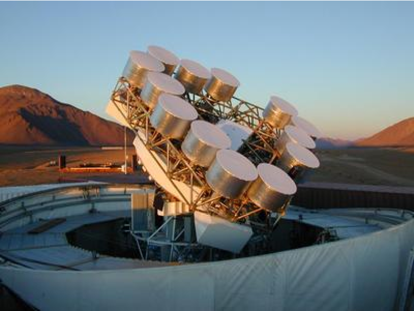
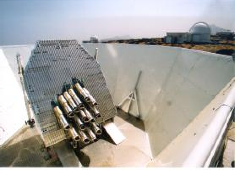
The CBI, shown in Figure 1, was the first of the new generation of CMB interferometers to be brought into operation (Padin et al. 2001), in January 2000. At that time the CBI began routine total intensity observations as well as preliminary polarization observations using a single cross-polarized antenna. We describe the CBI here in some detail since both the DASI and the VSA share most of these characteristics, and we point out the principal features in the VSA and the DASI in which they differ from the CBI. All three instruments operate in the Ka waveguide band (26 – 40 GHz) and use low-noise amplifiers (LNAs) based on high electron mobility transistors (HEMTs), which were designed by Marian Pospieszalski of the National Radio Astronomy Observatory (Pospieszalski et al. 1994, 1995). The specifications of the three instruments are given in Table 1.

As described by Padin et al. (2002), the CBI has 13 90-cm diameter antennas mounted on a 6-m platform. In addition to the usual altazimuth rotation axes, the CBI platform can be rotated about the optical axis. This third axis of rotation enables the array to maintain a constant parallactic angle while tracking a celestial source; it also greatly facilitates polarization observations and calibration, and, in addition, it provides a powerful method of discriminating between sky signals and instrumental cross-talk. For each baseline both the real and imaginary channels are correlated in a complex correlator, and there are 10 1-GHz bandwidth frequency channels spanning the range 26–36 GHz. Thus, the CBI comprises a total of 780 complex interferometers. The fundamental data rate is 0.84 s. For typical total intensity observations the data are averaged over 10 samples, so that on each interferometer the complex visibility is measured every 8.4 s.

Figure 2: The aperture-plane, (u,v), coverage of the CBI for a 6-hour observation. The left-hand panel shows the coverage for a single channel, and the right-hand panel shows the coverage for all 10 channels.

Figure 3: The CBI has made mosaic observations of three regions separated by 6 hr in Right Ascension. Mosaic images from the first year of observations, which cover an area of $\sim 2^{\circ}\times 2^{\circ}$, are shown above. In these images the seeds that gave rise to clusters of galaxies are seen for the first time.

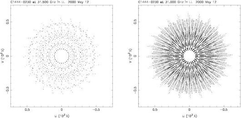
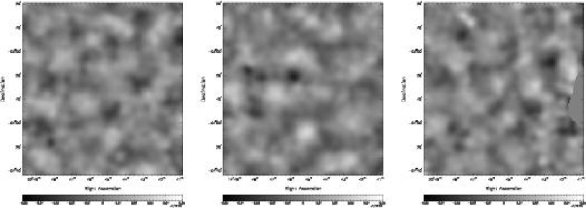
The aperture-plane, or (u,v), coverage of the CBI is shown in Figure 2. In this figure the (u,v) coverage corresponding to a single baseline should be the convolution of two apertures centered on the (u,v) point corresponding to the baseline length and orientation. For clarity we have shrunk the aperture convolution to a single point to make the distribution of the coverage clearer. There is, of course, much overlap in the coverage when the full diameters are used, since the antenna diameter of 90 cm is close to the size of the shortest baselines (100 cm). Mosaic observations of contiguous fields improve the resolution in multipole space. For example, in the CBI, mosaic observations have been used to improve the multipole resolution from $\delta l\approx 500$ to $\delta\approx 140$. CBI mosaic observations of three fields are shown in Figure 3.

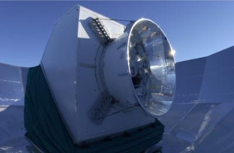
The DASI is shown in Figure 4. The DASI was designed to complement the CBI in multipole coverage, and many of the detailed CBI designs, including those for the correlator, the receiver control cards, and the channelizer, as well as the telescope control and data acquisition software, were shared with the DASI team, who duplicated these components in the DASI. For these reasons, the DASI is in many respects a copy of the CBI, but $\sim$ 4 times smaller. The DASI achromatic polarizers were duplicated by the DASI team for use on the CBI in its upgraded phase for full polarization observations, which commenced in October 2002. The DASI observed in total intensity mode during the austral winter of 2000, and was then outfitted with achromatic polarizers and both a ground screen and a sunscreen, shown in Figure 4, for the austral winter of 2001 when it made polarization observations of two fields, as described by Zaldarriaga (2003).

Figure 4: The Degree Angular Scale Interferometer (DASI), located at 2800 m at the South Pole, was outfitted with a sunscreen for the polarization observations of 2001.

Figure 5: The Very Small Array (VSA) is sited at 2400 m in Tenerife.

The VSA (Figure 5) and the DASI are similar in size, and originally covered similar multipole ranges (and hence very similar angular scales), extending from $l\approx 150$ to $l\approx 900$ with a resolution in multipoles of $\delta l\approx 80$. In 2001 the original VSA horns were replaced with a larger set that extended the VSA range up to $l\approx 1400$.

The CBI covers the range $l\approx 300$ to $l\approx 3500$ with a multipole resolution in mosaicing mode of $\delta l\approx 140$. Apart from this primary difference in multipole range and resolution, the other major difference is in the correlators — the CBI and the DASI each have 10 1-GHz channels, operating between 26 GHz and 36 GHz, while the VSA has a single tunable 1.5-GHz channel, which operates over the same frequency range.

3 The Sky Brightness Distribution of the CMB

We denote the CMB temperature in direction ${\bf\hat{n}}$ (angular coordinates $\theta,\phi$) by $T({\bf\hat{n}})$, and hence the variation in temperature about the mean $\langle T({\bf\hat{n}})\rangle$ by

$$\Delta({\bf\hat{n}})={T({\bf\hat{n}})\over{\langle T({\bf\hat{n}})\rangle}}-1,$$ (1)

which may be expanded into spherical harmonics

$$\Delta({\bf\hat{n}})=\sum_{l=0}^{\infty}\sum_{m=-l}^{l}a_{lm}Y_{lm}({\bf\hat{n}}),$$ (2)

where $a_{lm}$ are the multipole moments

$$a_{lm}=\int Y_{lm}^{*}({\bf\hat{n}})\Delta({\bf\hat{n}})d\Omega\quad.$$ (3)

If the CMB is isotropic it must be rotationally invariant so that the fluctuations can be expressed in terms of a one-dimensional angular spectrum, $C_{l}\equiv\langle a_{lm}^{2}\rangle$, and the variance of $\Delta({\bf\hat{n}})$ can be expressed in terms of this angular power spectrum:

$$\langle\Delta({\bf\hat{n}})^{2}\rangle=\sum_{l=0}^{\infty}{2l+1\over{4\pi}}C_{l}\quad.$$ (4)

For large $l$,

$$\langle\Delta({\bf\hat{n}})^{2}\rangle\approx\int{l(2l+1)\over{4\pi}}C_{l}\;d\,{\rm ln}\,l,$$ (5)

showing that the contribution to the variance from a logarithmic interval of $l$ is proportional to $l(2l+1)C_{l}/4\pi$. It is therefore often convenient to plot this quantity versus log$\,l$, so this convention is adopted by many authors in displaying angular spectra of the CMB. It should be borne in mind, however, that the signal is $C_{l}$, so that, in plotting $l(2l+1)C_{l}/4\pi$ we are artificially boosting the apparent variance at high $l$ by a factor $\propto l^{2}$. Observations at high $l$ therefore require far greater sensitivity than is immediately apparent from this conventional way of plotting the angular power spectrum.

The angular correlation function is defined as

$$C(\theta)=C({\bf\hat{n}_{1}},{\bf\hat{n}_{2}})=\langle\Delta({\bf\hat{n}_{1}})\Delta({\bf\hat{n}_{2}})\rangle,$$ (6)

where by isotropy and homogeneity $C$ is a function only of $\theta$, and $\cos\theta={\bf\hat{n}_{1}}\cdot{\bf\hat{n}_{2}}$. It is easy to show that

$$C(\theta)={1\over{4\pi}}\sum_{l=0}^{\infty}(2l+1)C_{l}P_{l}(\cos\theta),$$ (7)

where $P_{l}(\cos\theta)$ is the Legendre polynomial. The inverse result is

$$C_{l}=2\pi\int_{-1}^{1}C(\theta)P_{l}(\cos\theta)d\,\cos\,\theta\quad.$$ (8)

These two results are the analogs on the sphere of the theorem relating the covariance function to the Fourier transform of the power spectrum.

In interferometric observations of the CMB the fields of view, even for mosaic observations, are small enough that the small-angle approximation may be used. That is, we can assume that

$$\theta\ll 1\;\;{\rm and}\;\;l\gg 1.$$ (9)

In this case

$$P_{l}(\cos\theta)\approx J_{0}\{(l+{1/2})\;\theta\},$$ (10)

so that

$$C_{l} \approx 2\pi\int_{-1}^{1}C(\theta)J_{0}\{(l+{1/2})\;\theta\}d\,\cos\,\theta$$ (11)

$$\approx 2\pi\int_{0}^{\infty}C(\theta)J_{0}\{(l+{1/2})\;\theta\}\,\theta\,d\,\theta\quad.$$

If we set $l+1/2=2\pi v$ then this is a Hankel transform, which is simply the two-dimensional Fourier transform for a circularly symmetric function; i.e., as expected, the angular correlation function and the power spectrum form a Fourier transform pair in the small-angle approximation.

In practice we observe the sky with instruments of finite size, so that what we observe is the convolution of the sky brightness distribution with the instrument response function, corresponding to a product in the Fourier transform (spectral) domain:

$$C(\theta)={1\over{4\pi}}\sum_{l=0}^{\infty}(2l+1)C_{l}W_{l}(\cos\theta),$$ (12)

where $W_{l}(\cos\theta)$ is called the window function of the instrument.

4 Radio Interferometric Observations of the CMB

We do not review here the basic theory of radio interferometry, but refer the reader to the comprehensive text of Thompson, Moran, & Swenson (2001). Useful discussions of the application of standard radio interferometric techniques to observations of the CMB have been given by Hobson, Lasenby, & Jones (1995), White et al. (1999), Hobson & Maisinger (2002), and Myers et al. (2003).

Figure 6: The Multiplying Interferometer subtracts off the constant term in the field under observation, as was first demonstrated by Martin Ryle in 1952 (see text).

5 Interferometer Characteristics

The following properties of interferometers make them particularly well suited to observations of the CMB:

• Automatic subtraction of the mean signal (to high precision)

• Precise knowledge of the beamshape is easy to obtain (and is not as important as it is in single-dish observations)

• Direct measurements of visibilities (which are very nearly the desired Fourier components of the sky brightness distribution)

• Precision radiometry (through observations of planets, supernova remnants, quasars, and radio galaxies)

• Precision polarimetry (and, in the case of the CBI, making use of the third axis of rotation about the optical axis)

• Repeated baselines enable a wide variety of instrumental crosschecks

We discuss each of these interferometer properties separately below, illustrating some of them with examples from the CBI. It should be clear that similar advantages apply, in most cases, to the DASI and the VSA.

1 Automatic Mean Subtraction

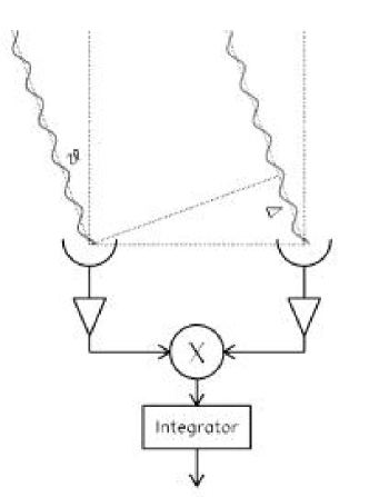
A multiplying interferometer (Fig. 6) has the advantage over adding interferometers and other total-power detection systems in that the mean signal is subtracted automatically to high precision (Ryle 1952). In the adding interferometer the voltages from the two antennas are added and then squared in a square-law detector, so that the power output from the square-law detector is proportional to $(V_{1}+V_{2})^{2}$. Ryle introduced the phase-switched interferometer in which the voltages are alternately summed and differenced by introducing a $\pi/2$ phase offset in one of the signals, and then detected by a phase-synchronous detector, which is in phase with the phase switch. In this system the output power is the time average of $(V_{1}+V_{2})^{2}-(V_{1}-V_{2})^{2}$, and so it is proportional the the product of the voltages from the two antennas. The power output in this system is thus independent of the mean level of the signal, $V_{1}^{2}+V_{2}^{2}$, and it measures the correlation between the two signals, $\langle V_{1}V_{2}\rangle$. Modern interferometers, such as those discussed here, accomplish the same effect by using a correlator. Since, in a multiplying or phase-switching interferometer, the mean signal does not appear, and only the spatially varying signal appears, this eliminates many sources of spurious systematic errors. This approach is particularly advantageous in CMB observations, in which the spatial fluctuations in temperature are over $10^{5}$ times smaller than the mean signal of 2.725 K (Mather et al. 1999). For this reason a number of potential sources of systematic error are reduced to negligible levels by interferometry.

Figure 7: Radial profile of the CBI primary beam in one of the 10 frequency channels; data from all 78 baselines are superimposed. The observations were of Tau A and are shown by the error bars. The curve shows the profile computed by taking the square of the Fourier transform of the aperture illumination pattern, assumed to be circularly symmetric. These observations show that the 13 antennas have very similar beams (see Pearson et al. 2003).

2 Precise Knowledge of Beamshape

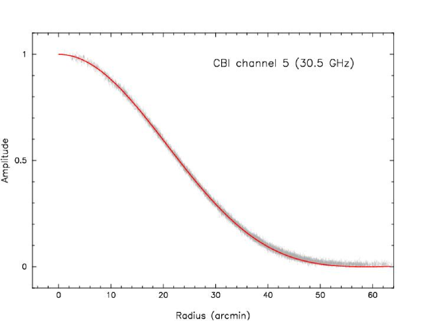
The resolution of an interferometer is set by the baseline length between the antenna pair, rather than by the primary beam of the individual antennas. Thus, in interferometric observations precise knowledge of the primary beamshape is not required in order to measure the power spectrum on small angular scales. Of course, precise knowledge of the primary beamshape is needed in computing the covariance function of the instrument, but this can be determined to the required accuracy of a few percent by measurements of the beamshape on bright unresolved radio sources. The profile of the mean primary beamshape for the CBI is shown in Figure 7.

3 Direct Measurements of Visibilities

An interferometer measures visibility, which is the Fourier transform of the product of the primary antenna beam, $A({\bf x})$, with the sky brightness, $I({\bf x})$. The visibilities, $V({\bf u})=V(u,v)$, measured by an interferometer are related to the sky brightness by

$$V({\bf u})=\int_{-\infty}^{\infty}\int_{-\infty}^{\infty}A({\bf x})I({\bf x})\,e^{-2\pi i{\bf u}\cdot{\bf x}}d{\bf x}\quad.$$ (13)

Figure 8: Panels (a) and (c) illustrate two multipole components of the sky brightness distribution over a $1.5^{\circ}\times 1.5^{\circ}$ field of view, typical for the CBI. An interferometer measures directly these components multiplied by the primary beam, which is fixed by the antenna size and illumination. The product of the primary beam with the multipole component measured by an interferometer, which is set by the baseline length, is shown for the two multipole components above in panels (b) and (d). In the case of the CBI, (a) and (b) represent the one-meter baselines, while (c) and (d) represent the five-meter baselines.

The visibility is thus the convolution of the Fourier transform of the sky brightness, $\tilde{I}({\bf u})$ (i.e., the angular spectrum of the sky brightness distribution), and of the primary beam, $\tilde{A}({\bf u})$,

$$V({\bf u})=\tilde{I}({\bf u})*\tilde{A}({\bf u})\quad.$$ (14)

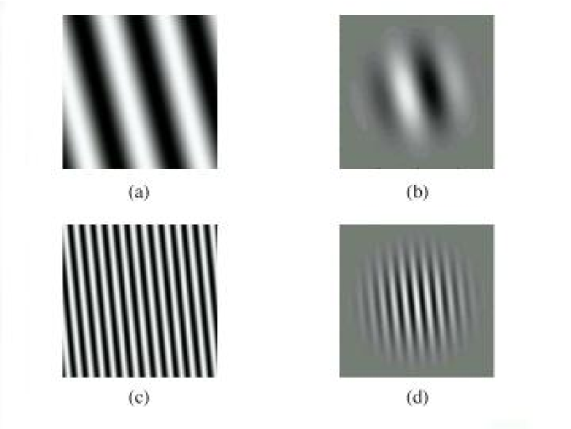
An interferometer therefore measures directly the angular spectrum of the sky brightness distribution, which is the desired result, convolved with the Fourier transform of the primary beam. An example of a single Fourier component on the sky and of this component multiplied by the primary beam is shown in Figure 8.

The matrix of the covariance between all the visibility measurements is the observed covariance matrix, $C_{ij}=\langle V_{i}V_{j}^{*}\rangle$, and this is made up of two parts,

$${\bf C=M+N},$$ (15)

where ${\bf M}$ is the sky covariance matrix and ${\bf N}$ is the noise covariance matrix. Hobson et al. (1995) have shown that the sky covariance matrix is

$$M_{jk} = \langle V({\bf u}_{j},\nu_{j})V^{*}({\bf u}_{k},\nu_{k})\rangle$$ (16)

$$= \int\int d^{2}{\bf v}\tilde{A}({\bf u}_{j}-{\bf v},\nu_{j})\tilde{A}({\bf u}_{k}-{\bf v},\nu_{k})S({\bf v},\nu_{j},\nu_{k}),$$

where $S({\bf v},\nu_{j},\nu_{k})$ is a generalized power spectrum of the intensity fluctuations. Hence, converting to temperature fluctuations, we find that for CMB fluctuations,

$$M_{jk} = \langle V({\bf u}_{j},\nu_{j})V^{*}({\bf u}_{k},\nu_{k})\rangle$$ (17)

$$= \left({2\nu^{2}k_{B}T_{0}g(\nu)\over c^{2}}\right)^{2}\int\int d^{2}{\bf v}\tilde{A}({\bf u}_{j}-{\bf v},\nu_{j})\tilde{A}({\bf u}_{k}-{\bf v},\nu_{k})C(v)$$

$$= \left({2\nu^{2}k_{B}T_{0}g(\nu)\over c^{2}}\right)^{2}\int_{0}^{\infty}W_{jk}(v)C(v)vdv,$$

where $g(\nu)=x^{2}e^{x}/(e^{x}-1)^{2}$, $x=h\nu/k_{B}T_{0}$, and $C(v)=C_{l}$ for $\sqrt{l(l+1)}\approx l+{1\over 2}=2\pi v$, and

$$W_{jk}(v)=\int_{0}^{2\pi}\tilde{A}({\bf u}_{j}-{\bf v},\nu_{j})\tilde{A}({\bf u}_{k}-{\bf v},\nu_{k})d\theta_{v}$$ (18)

is the window function.

4 Precision Radiometry

A great advantage of interferometric measurements is precision radiometry. Provided that there are sufficiently bright unresolved and nonvarying radio sources, the calibration of interferometers is straightforward. In the case of the CBI, for example, the primary calibrators were Jupiter and Tau A, and secondary calibrators were Mars, Saturn, and 3C 274. Of these only Tau A is significantly resolved on the CBI, but it is easily modeled with an elliptical Gaussian brightness profile. The internal calibration consistency on the CBI is considerably better than 1%, and the flux density scale, originally set by our own absolute calibrations at the Owens Valley Radio Observatory with an uncertainty of 3.3% (Mason et al. 1999), has now been improved by comparison with the WMAP temperature measurement of Jupiter (Page et al. 2003) to an uncertainty of 1.3% (Readhead et al. 2003).

5 Precision Polarimetry

The instrumental polarization of radio interferometers is much easier to calibrate than single-dish instruments, because there is an elegant way of distinguishing between the polarization of the instrument and that of the source (Conway & Kronberg 1969). The instrumental polarization can be expressed in terms of leakage factors. In the CBI each antenna observes either left- or right-circular polarization. The voltage output from a left-circularly polarized antenna, $p$, may be written

$$V_{L}(p)=E_{L}(p)+E_{R}(p)\epsilon_{p}e^{j\phi_{p}},$$ (19)

where $E_{L}(p)$ is the electric field that we wish to measure, and $\epsilon_{p}e^{j\phi_{p}}$ represents the instrumental leakage of the unwanted right-circular polarization electric field, $E_{R}(p)$, on antenna $p$. Similarly, the voltage output of a right-circular polarized antenna, $q$, may be written

$$V_{R}(q)=E_{R}(q)+E_{L}(q)\epsilon_{q}e^{j\phi_{q}},$$ (20)

where $\epsilon_{q}e^{j\phi_{q}}$ represents the instrumental leakage of left-circular polarization on antenna $q$.

For a point source with zero circular polarization the correlator output on the LR cross-polarized baselinem which combines antenna $p$ with antenna $q$, can be written

$$V_{L}(p)V_{R}^{*}(q) = {E_{L}(p)E_{R}^{*}(q)e^{2j\eta}+I(\epsilon_{p}e^{j\phi_{p}}+\epsilon_{q}e^{-j\phi_{q}})\over{(1+\epsilon_{p}^{2})^{1/2}(1+\epsilon_{q}^{2})^{1/2}}}$$ (21)

$$= {mIe^{2j\chi}e^{2j\eta}+I(\epsilon_{p}e^{j\phi_{1}}+\epsilon_{q}e^{-j\phi_{2}})\over{(1+\epsilon_{p}^{2})^{1/2}(1+\epsilon_{q}^{2})^{1/2}}},$$

where $m$ is the linear polarization, $I$ is the total intensity, $\chi$ is the polarization angle on the sky, and we have neglected terms of order $\epsilon^{2}$ and higher. The angle $\eta$ is the azimuthal angle of the antennas about the line of sight to the source. In the CBI and the DASI, the antennas are mounted on a rotatable deck, so that, in addition to the usual two (alt-az) axes, the instruments can be rotated about the optical axis, thereby varying $\eta$ for all antennas simultaneously. The expression given above applies for instruments such as the CBI and the DASI in which a single rotation by $\eta$ of the deck upon which the antennas are all mounted leads to a phase advance of $\eta$ in one polarization and a phase retardation of $\eta$ in the other polarization — thereby giving rise to a relative phase shift of $2\eta$ on cross-polarized baselines.

By means of rotation of the deck, it is easy to measure the instrumental polarization on an instrument such as the CBI or the DASI: we simply need to observe a bright unresolved polarized source, for which $m$ and $\chi$ are known, such as 3C 279, and measure $V_{L}(p)V_{R}^{*}(q)$ while varying $\eta$ by rotating the deck. The complex number $V_{L}(p)V_{R}^{*}(q)$ then traces out an ellipse that is closely approximated by a circle of radius

$$mI/(1+\epsilon_{p}^{2})^{1/2}(1+\epsilon_{q}^{2})^{1/2}$$ (22)

centered on the point

$${I(\epsilon_{p}e^{j\phi_{p}}+\epsilon_{q}e^{-j\phi_{q}})\over{(1+\epsilon_{p}^{2})^{1/2}(1+\epsilon_{q}^{2})^{1/2}}}\quad.$$ (23)

By observing a bright source of known polarization on all baselines, it is then possible to solve for the individual antenna leakage factors to high precision. Both the CBI and the DASI use achromatic polarizers with leakage factors $<3\%$ designed by John Kovac (Kovac et al. 2002), so that, after correcting for instrumental polarization, uncertainties in polarization due to instrumental effects are $\ll 1\%$.

The polarization of the CMB can be expressed in terms of a curl-free mode and a curl mode. By analogy with electromagnetic theory these are designated as the $E$-mode and the $B$-mode. The strongest polarized signal in the CMB is due to Thomson scattering by electrons of the anisotropic radiation field due to quadrupole velocity anisotropy, and this is an $E$-mode component. The much weaker $B$-mode components would be caused by gravitational radiation or gravitational lensing (see, e.g., Hu 2003).

It can be shown that for the case of infinitely small antennas the sum of the LR+RL visibilities yields the Fourier transform of the $E$-mode, while the difference LR$-$RL yields the Fourier transform of the $B$-mode (Zaldarriaga 2001). For the realistic case of finite antennas there is also a small amount of mixing of these modes due to the finite aperture. This is a direct analog of the arguments given above showing that the visibility in total intensity is the convolution of the angular spectrum with the Fourier transform of the primary beam.

6 Instrumental Crosschecks

On the CBI there are many duplicated baselines in any given orientation of the deck, and further baseline duplication can be accomplished by deck rotation. This is very useful in tracking down and eliminating various sources of systematic errors (e.g., cross-talk between electronic components). It also provides for crosschecks of visibilities on calibrators measured on different baselines, etc.

6 CMB Spectra from Interferometry Observations

The CBI began CMB observations at the Chilean site in January 2000, and the DASI and the VSA began their observations shortly thereafter. In this section we discuss the details of the spectra revealed by these interferometric observations, and in the following section we discuss the constraints that these place on key cosmological parameters.

Figure 9: The mass of material within a sphere at the last-scattering surface is shown as a function of the angular diameter of the sphere. Here we have assumed a $\Lambda$CDM model in which $\Omega_{\rm matter}\,h^{2}=0.3$ and $\Omega_{\rm total}=1$. The mass scales accessed by various CMB observations are shown. Only the CBI and ACBAR cover masses of galaxy clusters.

Figure 10: The CBI spectrum shown here was obtained with a combination of deep observations of single fields and mosaic observations of $2^{\circ}\times 4^{\circ}$ fields. The results for two alternate binning schemes are shown by the solid error bars and closed circles, and the dashed error bars and open circles. These are not independent points, but there is more information in the data than can be displayed in a single spectrum, and this also shows that there is nothing peculiar about the particular binning scheme being used. The spectrum shows four important features for the first time: (1) anisotropy on multipoles above $l\approx 1000$, corresponding to mass scales typical of clusters of galaxies; (2) the damping tail due to photon viscosity in the scattering region and the finite thickness of this region; (3) the second, third, and fourth acoustic peaks, with strong hints of the first and fifth peaks; and (4) an excess of power in the multipole range $2000<l<3500$, ascribed to the Sunyaev-Zel’dovich effect in either galaxy clusters or the ionized regions produced by Population III stars (see text).

1 The CBI CMB Spectrum

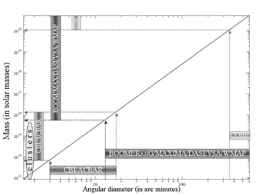
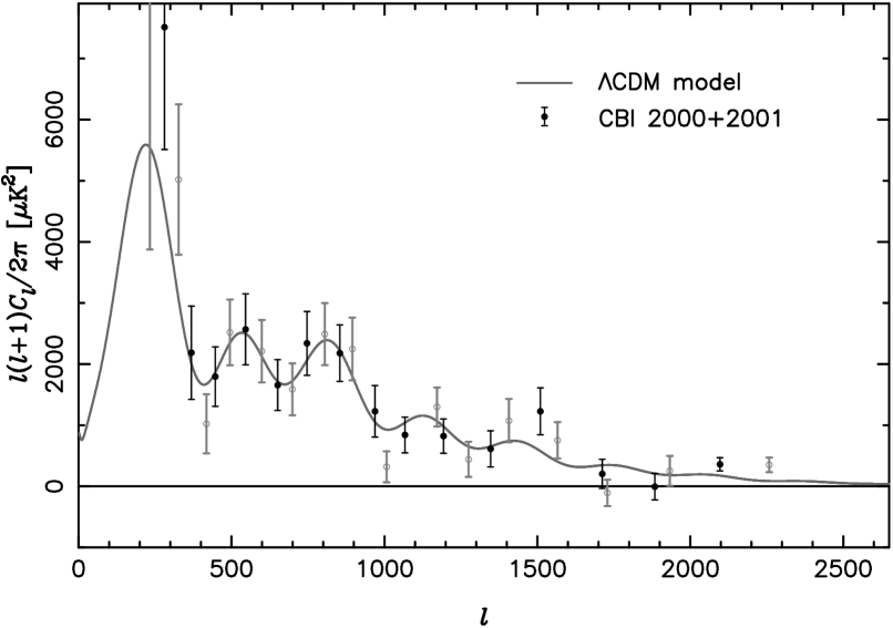
The first results from the new generation of interferometers were published by the CBI group in January 2001. These were the first observations of the CMB with both the sensitivity and the resolution to make images of the mass fluctuations on scales corresponding to clusters of galaxies (Padin et al. 2001; Mason et al. 2003; Pearson et al. 2003), and the images show clearly, and for the first time, the seeds that gave rise to galaxy clusters (Fig. 3). The straight line in Figure 9 shows the mass within a spherical region at the epoch of last scattering as a function of the angular diameter of the sphere, assuming a $\Lambda$CDM cosmology. Also shown are the angular scales and the corresponding mass scales that have been probed by key CMB experiments over the last three years. In addition, these were the first CMB observations to show the reduction in spectral power at high multipole numbers due to the damping tail at small scales caused by photon viscosity and the finite thickness of the last-scattering region. Thus, this major pillar of the standard $\Lambda$CDM cosmology has been confirmed by the CBI observations. The CBI spectrum for observations from January 2000 through November 2001 is shown in Figure 10.

An intriguing feature of the CBI spectrum is the excess of power seen at $l\approx 2500$ (Mason et al. 2003). The reality of this feature and its possible significance are discussed below.

At the frequency of operation of the CBI (26 – 36 GHz), and at multipoles above $l\approx 500$, there is significant foreground contamination due to radio galaxies and quasars. These are dealt with in the CBI data by a constraint matrix approach, such as was first used on interferometry data by the DASI (Leitch et al. 2002a), and which effectively “projects out” the point sources. The application to the CBI is described in detail by Mason et al. (2003). Thus far it has been necessary to use the 1.4 GHz NRAO VLA Sky Survey (NVSS) (Condon et al. 1998) for identifying possible contaminating sources, because there is no higher-frequency radio survey that covers the CBI fields. Only $\sim 20\%$ of the NVSS sources are flat-spectrum objects that are bright enough at the CBI frequencies to cause detectable contamination, and a survey of NVSS sources in the CBI fields at $\sim 30$ GHz would enable us to identify these sources, thus reducing by a factor of 5 the number of sources that must be projected out of the CBI data. This would significantly increase the amount of CBI data that is retained, and it would substantially reduce the uncertainties in the CBI spectrum at multipoles higher than $l\approx 1000$. It is possible to measure the flux densities of the NVSS sources in the CBI frequency range with either the Bonn 100-m telescope or with the Green Bank Telescope.

Figure 11: The DASI spectrum. The symbols are as for the caption to Figure 10.

Figure 12: The VSA spectrum shown above was obtained by combining results from the first and second sets of horns (see text). The symbols are as for the caption to Figure 10.

In 2002 the CBI was upgraded with the DASI-style achromatic polarizers, and the antennas were moved into a close-packed configuration that concentrates the observations into the multipole range $500<l<2000$. Since October 2002 it has been observing in this configuration.

2 The DASI CMB Spectrum and the Detection of Polarized CMB

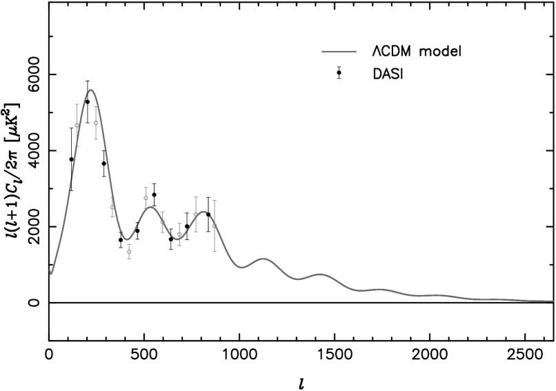
The first DASI results were released in April 2001 (Halverson et al. 2002). The DASI spectrum is shown in Figure 11. We see here a clear detection of the first and second acoustic peaks, and a hint of the third peak. These DASI results were the first interferometry results to show the first acoustic peak, which had first been seen clearly in the TOCO observations and then with very high signal-to-noise ratio in the BOOMERanG results released in April 2000 (de Bernardis et al. 2000).

In the second year of operation (2001) the DASI was outfitted with achromatic polarizers and carried out polarization observations that yielded a detection of polarized emission attributed to the CMB (Kovac et al. 2002; Leitch et al. 2002b). Thus, another key pillar of the standard cosmological model has been confirmed by an interferometer. The DASI polarization results are discussed in the article by Zaldarriaga (2003) in this volume.

3 The VSA CMB Spectrum

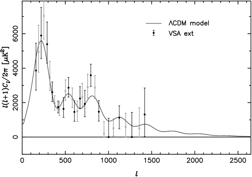
The VSA was deployed in 2000 with a compact array (Scott et al. 2003; Watson et al. 2003), and the following year the horns were replaced with larger ones and the array was extended to longer baselines, thereby permitting the VSA to make observations of the CMB spectrum up to multipoles $l\approx 1400$. The VSA CMB spectrum from the combination of observations with the original and extended arrays is shown in Figure 12 (Grainge et al. 2003; Scott et al. 2003). Here we can see clearly the first, second and third acoustic peaks.

Figure 13: The combined CBI, DASI, and VSA spectra show the excellent agreement between these three experiments in the region of overlap. The combination of these three spectra provides stringent constraints on key cosmological parameters and shows a number of the key spectral features predicted by theory: a large first acoustic peak followed by successively smaller harmonics of this peak, with a strong damping tail. The excess detected by the CBI at $l\approx 2500$ was not predicted and must be confirmed (see text).

Table 2: Cosmological Constraints from CMB Interferometers^†

Parameter	${\rm CBI}$	${\rm DASI}$	${\rm VSA}$	${\rm CBI+DASI+VSA}$
$\Omega_{\rm k}$	$-0.10_{-0.008}^{+0.007}$	$-0.06_{-0.05}^{+0.05}$	$-0.07_{-0.08}^{+0.08}$	$-0.06_{-0.04}^{+0.04}$
$n_{\rm s}$	$1.03_{-0.07}^{+0.10}$	$1.03_{-0.07}^{+0.12}$	$1.07_{-0.08}^{+0.10}$	$0.98_{-0.05}^{+0.08}$
$\Omega_{\rm cdm}\;h^{2}$	$0.11_{-0.03}^{+0.05}$	$0.12_{-0.03}^{+0.04}$	$0.17_{-0.05}^{+0.06}$	$0.12_{-0.02}^{+0.03}$
$\Omega_{\rm b}\;h^{2}$	$0.040_{-0.014}^{+0.013}$	$0.023_{-0.004}^{+0.004}$	$0.034_{-0.007}^{+0.007}$	$0.024_{-0.003}^{0.004}$
$\Omega_{\Lambda}$	$0.62_{-0.23}^{+0.15}$	$0.58_{-0.22}^{+0.16}$	$0.43_{-0.25}^{+0.22}$	$0.58_{-0.17}^{+0.14}$

^†Weak prior.

Table 3: Cosmological Constraints from CMB Interferometers^†

Parameter	${\rm CBI}$	${\rm DASI}$	${\rm VSA}$	${\rm CBI+DASI+VSA}$
$n_{\rm s}$	$0.99_{-0.06}^{+0.08}$	$1.00_{-0.06}^{+0.08}$	$1.05_{-0.07}^{+0.11}$	$0.96_{-0.04}^{+0.05}$
$\Omega_{\rm cdm}\;h^{2}$	$0.15_{-0.04}^{+0.04}$	$0.14_{-0.03}^{+0.03}$	$0.19_{-0.05}^{+0.05}$	$0.13_{-0.02}^{+0.03}$
$\Omega_{\rm b}\;h^{2}$	$0.028_{-0.009}^{+0.010}$	$0.022_{-0.003}^{+0.004}$	$0.031_{-0.006}^{+0.006}$	$0.023_{-0.003}^{+0.003}$
$\Omega_{\Lambda}$	$0.57_{-0.29}^{+0.18}$	$0.59_{-0.26}^{+0.16}$	$0.46_{-0.28}^{+0.22}$	$0.66_{-0.20}^{+0.11}$

^†Flat + weak priors.

7 Cosmological Results

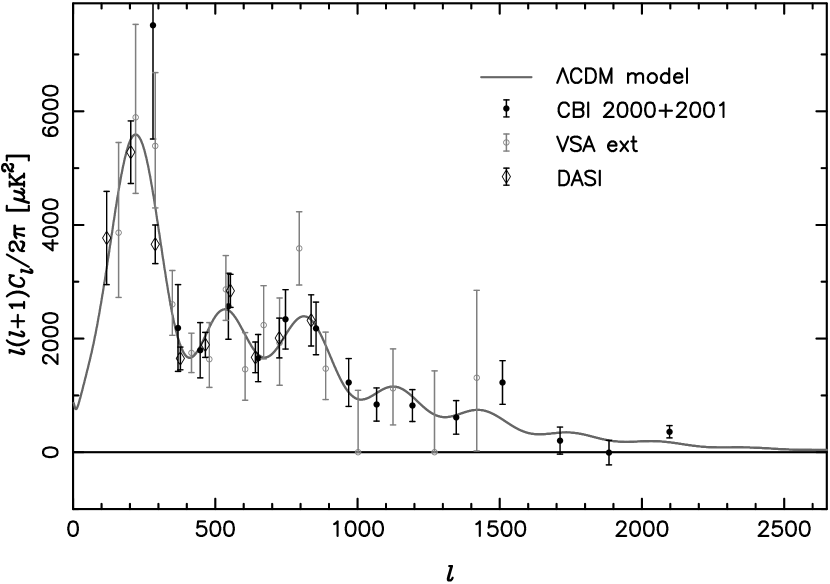
The CBI, DASI, and VSA CMB spectra are shown in Figure 13 (Halverson et al. 2002; Grainge et al. 2003; Pearson et al. 2003; Readhead et al. 2003). Here, in order to avoid confusion, we have plotted only a single binning of the data from each instrument, but the reader should be aware that there is considerably more information than can be displayed in this one-dimensional plot. There is excellent agreement between these three independent experiments in the regions of overlap. Some of the key cosmological results from these three interferometers are given in Table 2. The “weak prior” assumptions used here are that the age of the Universe is greater than 10 billion years, $45{\rm\;km\,s^{-1}\,Mpc^{-1}}\,<H_{0}\,<\,\,90\,\;{\rm km\,s^{-1}\,Mpc^{-1}}$, and $\Omega_{\rm matter}>0.1$. It can be seen that all three interferometers provide strong evidence for a flat geometry ($\Omega_{\rm k}\approx 0$) and a scale-invariant spectrum ($n_{\rm s}\approx 1$), both of which are expected for inflationary universes. Given the strong evidence here for a flat geometry, we have also determined key parameters for the case of a flat Universe, with the results shown in Table 3, where it can again be seen that the results are in excellent agreement, and it is clear that the matter density is only about one-third of the critical density, with the predominant matter component being nonbaryonic. Thus, the remainder of the energy density must be made up of something other than matter, and is here attributed to the cosmological constant. It is interesting to compare the CBI results, which depend almost entirely on high multipoles ($l>600$), and are therefore independent of the first peak, with the DASI and VSA results, which depend entirely on low multipoles, especially on the first peak. We see that the cosmological parameter values derived from both the DASI and the VSA agree very well with those derived from the CBI. This provides strong justification for the assumption of a featureless, primordial density fluctuation spectrum.

This is important because it is conceivable that the structures observed in these angular spectra are not simply acoustic peaks, but contain significant features that are either present in the primordial spectrum or are produced by other, as yet undetermined, physical effects. If this were the case there could be significant errors in the derived cosmological parameters. However, it is almost inconceivable that we would derive the same incorrect cosmological parameters from two different parts of the angular spectrum. This conclusion has been strengthened by the recent ACBAR results (Goldstein et al. 2003), which cover much of the same range of multipoles as the CBI.

We have carried out an analysis of the CBI+WMAP observations in order to determine the additional constraints placed on cosmological parameters by the extension of the spectrum beyond the range covered by WMAP (Bennett et al. 2003; Readhead et al. 2003). The results are shown in Table 4. Comparison of this table with Tables 2 and 3 shows clearly the much tighter cosmological constraints from WMAP. It can be seen here, however, that the extension of the spectral coverage to high $l$ by the CBI yields a significant reduction in many of the parameter uncertainties.

Table 4: Cosmological Constraints from WMAP and from WMAP+CBI

Parameter	WMAP	WMAP+CBI
$\Omega_{\rm k}$	$-0.063_{-0.028}^{+0.050}$	$-0.071_{-0.023}^{+0.064}$
$n_{\rm s}$	$0.975_{-0.020}^{+0.032}$	$0.962_{-0.013}^{+0.022}$
$\Omega_{\rm cdm}\;h^{2}$	$0.125_{-0.0092}^{+0.015}$	$0.120_{-0.0092}^{+0.0072}$
$\Omega_{\rm b}\;h^{2}$	$0.0234_{-0.0008}^{+0.0012}$	$0.0231_{-0.0005}^{+0.0010}$
$\Omega_{\Lambda}$	$0.437_{-0.075}^{+0.243}$	$0.446_{-0.059}^{+0.289}$

1 The Spectrum above $l\approx 2000$

There is excellent agreement between all of the CMB observations in the regions of overlap, and these are well fitted by a $\Lambda$CDM model. At higher multipoles, however, the CBI results are not consistent with the predicted levels of the anisotropies, but show an excess that is significant at the $\sim 3\,\sigma$ level (Bond et al. 2003; Mason et al. 2003).

In the 2001 season the CBI concentrated on mosaic observations in order to increase the resolution in $l$, whereas deep observations of a small number of fields give the best sensitivity to observations at high $l$. Nevertheless, the 2001 observations do contribute to this region. The observations from 2000 alone yield a value of $508_{-149}^{+116}\,\mu{\rm K}^{2}$, which is an excess of 3.1 $\sigma$ over the predicted $\Lambda$CDM model in the multipole range $2000<l<3500$; whereas the observations from 2000 and 2001 combined yield $360_{-95}^{+102}\,\mu{\rm K}^{2}$, which is significantly lower in absolute terms. The resulting significance relative to the $\Lambda$CDM model has therefore dropped to 2.3 $\sigma$. The tantalizing detection of the excess persists, therefore, albeit at lower significance, in the combined 2000+2001 CBI data set (see Readhead et al. 2003), and more observations are required to confirm or disprove this excess.

If real, the excess at high multipoles detected by the CBI could have significant consequences, as has been spelled out in a number of papers (e.g., Bond et al. 2003; Oh, Cooray, & Kamionkowski 2003). Both of these papers ascribe the excess to the Sunyaev-Zel’dovich effect. The paper by Bond et al. attributes the excess to the Sunyaev-Zel’dovich effect in clusters of galaxies, while that of Oh et al. attributes it to the Sunyaev-Zel’dovich effect in hot gas resulting from supernova explosions in the first generation of stars (Population III). The WMAP results (Bennett et al. 2003) have shown that reionization started early, at around a redshift of 20, so it may be that both the CBI and WMAP results provide evidence for Population III stars.

8 Conclusions

The results from the three CMB interferometers show excellent agreement and provide compelling evidence for an approximately flat Universe with an approximately scale-invariant spectrum. The derived baryonic matter density is consistent with big bang nucleosynthesis calculations, and the total matter content is only $\sim$40% of the critical density required for a flat Universe. Therefore, it is clear that the major fraction of the energy density of the Universe is provided by something other than matter. This is generally assumed to be a nonzero cosmological constant.

The high-$l$ excess detected by the CBI, if real, is the most interesting result of the CMB interferometry experimental results. It is unexpected, and would likely be due to secondary anisotropy. Both the suggested explanations, that it is due to the Sunyaev-Zel’dovich effect in clusters of galaxies (Bond et al. 2003) or in the aftermath of Population III stars (Oh et al. 2003), would provide an important new window on the processes of structure formation.

References

- [1] Bennett, C., et al. 2003, ApJ, in press (astro-ph/0302207)
- [2] Bond, J. R., et al. 2003, ApJ, submitted (astro-ph/0205386)
- [3] Condon, J. J., Cotton, W. D., Greisen, E. W., Yin, Q. F., Perley, R. A., Taylor, G. B., & Broderick, J. J. 1998, AJ, 115, 1693
- [4] Conway, R. G., & Kronberg, P. P. 1969, MNRAS, 142, 11
- [5] de Bernardis, P., et al. 2000, Nature, 404, 955
- [6] Goldstein, J. H., et al. 2003, ApJ, submitted (astro-ph/0212517)
- [7] Grainge, K., et al. 2003, MNRAS, 341, L23
- [8] Halverson, N., et al. 2002, ApJ, 568, 38
- [9] Hanany, S., et al. 2000, ApJ, 545, L5
- [10] Hobson, M. P., Lasenby, A. N., & Jones, M. 1995, MNRAS, 275, 863
- [11] Hobson, M. P., & Maisinger, K. 2002, MNRAS, 334, 569
- [12] Hu, W. 2003, Annals of Physics, 303, 203
- [13] Kovac, J., Leitch, E. M., Pryke, C., Carlstrom, J. E., Halverson, N. W. & Holzapfel, W. L. 2002, Nature, 420, 720
- [14] Lee, A., et al. 2001, ApJ, 561, L1
- [15] Leitch, E. M., et al. 2002a, ApJ, 568, 28
- [16] ——. 2002b, Nature, 420, 763
- [17] Mason, B. S., et al. 2003, ApJ, in press (astro-ph/0205384)
- [18] Mason, B. S., Leitch, E. M., Myers, S. T., Cartwright, J. K., & Readhead, A. C. S. 1999, AJ, 118, 2908
- [19] Mather, J. C., Fixsen, D. J., Shafer, R. A., Mosier, C., & Wilkinson, D. T. 1999, ApJ, 512, 511
- [20] Myers, S. T., et al. 2003, ApJ, in press (astro-ph/0205385)
- [21] Netterfield, B., et al. 2002, ApJ, 571, 604
- [22] Oh, S. P., Cooray, A., & Kamionkowski, M. 2003, MNRAS, 342, L20
- [23] Padin, S., et al. 2001, ApJ, 549, L1
- [24] ——. 2002, PASP, 114, 83
- [25] Page, L., et al. 2003, ApJ, in press (astro-ph/0302214)
- [26] Pearson, T. J., et al. 2003, ApJ, in press (astro-ph/0205388)
- [27] Pospieszalski, M. W., et al. 1995, IEEE MTT-S International Symp. Digest, 95.3, 1121
- [28] Pospieszalski, M. W., Nguyen, L.D., Lui, T., Thompson, M. A., & Delaney, M. J. 1994, IEEE MTT-S International Symp. Digest, 94.3, 1345
- [29] Readhead, A. C. S., et al. 2003, in preparation
- [30] Ryle, M. 1952, Proc. Roy. Soc., 211, 351
- [31] Scott, P. F., et al. 2003, MNRAS, 341, 1076
- [32] Scott, P. F., Saunders, R., Pooley, G., O’Sullivan, C., Lasenby, A. N., Jones, M., Hobson, M. P., Duffet-Smith, P. J., & Baker, J. 1996, ApJ, 461, L1
- [33] Thompson, A. R., Moran, J. M. & Swenson G. W. 2001, Interferometry and Synthesis in Radio Astronomy, 2nd ed. (New York: Wiley)
- [34] Watson, R. A., et al. 2003, MNRAS, 341, 1057
- [35] White, M., Carlstrom, J. E., Dragovan, M., & Holzapfel, W. L. 1999, ApJ, 514, 12
- [36] Zaldarriaga, M. 2001, Phys. Rev. D, 64, 103001
- [37] ——. 2003, in Carnegie Observatories Astrophysics Series, Vol. 2: Measuring and Modeling the Universe, ed. W. L. Freedman (Cambridge: Cambridge Univ. Press), in press