Abstract

The Wilkinson Microwave Anisotropy Probe (WMAP) has mapped the full sky in five frequency bands between 23 and 94 GHz. The primary goal of the mission is to produce high-fidelity, all-sky, polarization-sensitive maps that can be used to study the cosmic microwave background. Systematic errors in the maps are constrained to new levels: using all-sky data, aspects of the anisotropy may confidently be probed to sub-$\mu$K levels. We give a brief description of the instrument and an overview of the first results from an analysis of maps made with one year of data. The highlights are (1) the flat $\Lambda$CDM model fits the data remarkably well, whereas an Einstein-de Sitter model does not; (2) we see evidence of the birth of the first generation of stars at $z_{r}\approx 20$; (3) when the WMAP data are combined and compared with other cosmological probes, a cosmic consistency emerges: multiple different lines of inquiry lead to the same results.

Chapter 0 The Wilkinson Microwave
Anisotropy Probe

1 Introduction

We present the first results from the Wilkinson Microwave Anisotropy Probe (WMAP), which completed its first year of observations on August 9, 2002. Dave Wilkinson, for whom the satellite was renamed, was a friend and colleague to many of the conference participants. He was a leader in the development of the cosmic microwave background (CMB) as a potent cosmological probe. He died on September 5, 2002, after battling cancer for 17 years, all the while advancing our understanding of the origin and evolution of the Universe. He saw the data in their full glory and was pleased with what I am able to report to you in the following.

At the time of the conference, the data were not ready to be released. The presentation focused on what WMAP would add to the considerable advances that had been made over the past few years. The emphasis was on the data; a companion talk by Ned Wright showed how the data are interpreted in the context of the currently favored models. Some effort was made to show what we knew firmly, like the position of the first acoustic peak in the CMB, as opposed to quantities that we knew better through the combination of multiple experiments, such as the characteristics of the second acoustic peak and the possible level of foreground contamination.

Since the conference, there have been 17 papers by the WMAP team describing the instrument and data. This contribution draws heavily from those papers. Bennett et al. (2003a) lay out the goals of the mission and give an overview of the instrument. More detailed descriptions of the radiometers, optics, and feed horns are found in Jarosik et al. (2003a), Page et al. (2003a), and Barnes et al. (2002). The inflight characterization of the receivers, optics, and sidelobes are described in Jarosik et al. (2003b), Page et al. (2003b), and Barnes et al. (2003). The data processing and checks for systematic errors are described by Hinshaw et al. (2003a), and Hinshaw et al. (2003b) present the angular power spectrum. Bennett et al. (2003c) present the analysis of the foreground emission. The temperature-polarization correlation is described in Kogut et al. (2003), and Komatsu et al. (2003) show that the fluctuations are Gaussian. Verde et al. (2003) present the details of the analysis of the angular power spectrum and show how the WMAP data can be combined with external data sets such as the 2dFGRS (Colless et al. 2001). Spergel et al. (2003) present the cosmological parameters derived from the WMAP alone, as well as the parameters derived from WMAP in combination with the external data sets. Peiris et al. (2003) confront the data with models of the early Universe, in particular inflation. The features in the power spectrum are interpreted in Page et al. (2003c). The scientific results are summarized in Bennett et al. (2003b).

Table 1: Characteristics of the Instrument

Band	$\nu_{center}$	$\Delta\nu_{noise}$	$N_{chan}$	$\Delta T/pix$	$\theta_{FWHM}$
	(GHz)	(GHz)		($\mu$K)	(deg)
K	23	5	2	20	0.82
Ka	33	7	2	20	0.62
Q	41	7	4	21	0.49
V	61	11	4	24	0.33
W	94	17	8	23	0.21

The $\Delta T/pix$ is the Rayleigh-Jeans sensitivity per $3.2\times 10^{-5}$ sr pixel for
the four-year mission for all channels of one frequency combined.

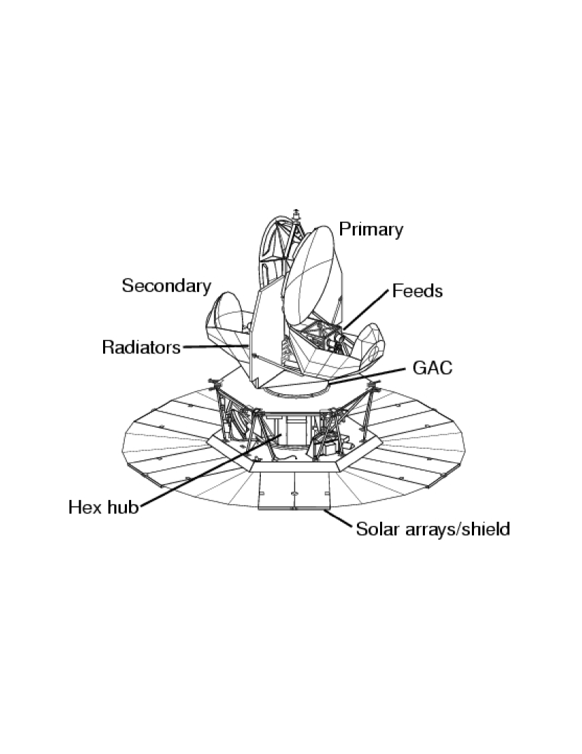
Figure 1: Outline of the WMAP satellite. The overall height is 3.6 m, the mass is 830 kg, and the diameter of the large disk on the bottom is 5.1 m. Six solar arrays on the bottom of this disk supply the 400 W to power the spacecraft and instrument. Thermal blanketing between the hex hub and GAC, and between the GAC and radiators, shield the instrument from thermal radiation from the support electronics and attitude control systems.

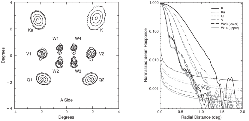
Figure 2: Left: The A-side focal plane obtained from observations of Jupiter. Note that the beam widths are a function of frequency. The farther a beam is from the central focus, the more ellipsoidal it is. In the V and W bands, the beams have substructure. This is due to deformations in the surface of the primary and was anticipated. The scan pattern symmetrizes all the beams. The contour levels correspond to 0.9, 0.6, 0.3, 0.09, etc. of the peak value. Right: The normalized, symmetrized beam response. Except in the K band, the beams are mapped to better than $-30$ dB of their peak value. The lower set of lines shows the noise level in the maps. From Page et al. (2003b).

2 Overview of the Mission and Instrument

The primary goal of WMAP is to produce high-fidelity, polarization-sensitive maps of the microwave sky that may be used for cosmological tests. WMAP was proposed in June 1995, at the height of the “faster, better, cheaper” era; some building began in June 1996, although the major push started in June 1997 after the confirmation review. WMAP was designed to be robust, thermally and mechanically stable, built of components with space heritage, and relatively easy to integrate and test.

There is no single thing on WMAP that sets the mission apart from other experiments. Rather, it is a combination of attributes that are designed to work in concert to take full advantage of the space environment. The mission goal is to measure the microwave sky on angular scales of $180^{\circ}$ as well as on scales of 0.^∘2 with micro-Kelvin accuracy. During the planning, building, and integration of the satellite, the emphasis was on minimizing systematic errors so that the data could be straightforwardly interpreted. There are many levels of redundancy that permit multiple cross-checks of the quality of the data.

WMAP was launched on June 30, 2001 into an orbit that took it to the second Earth-Sun Lagrange point, $L_{2}$, roughly $1.5\times 10^{6}~{}$km from Earth. The $L_{2}$ orbit is oriented so that the instrument is always shielded from the Sun, Earth, and Moon by the solar panels and flexible aluminized mylar/kapton insulation, as shown in Figure 1.1. The satellite has one mode of operation while taking scientific data. It spins and precesses at constant insolation, continuously measuring the microwave sky.

The instrument measures only temperature differences from two regions of the sky separated by roughly $140^{\circ}$. The instrument is composed of 10 symmetric, passively cooled, dual polarization, differential, microwave receivers. As shown in Table 1, there are four receivers in W band, two in V band, two in Q band, one in Ka band, and one in K band. The receivers are fed by two back-to-back Gregorian telescopes.

The instrument is passively cooled. The optics, shielded from Sun and Earth, radiate to free space and cool to 70 K. Two large (5.6 m² net) and symmetric radiators passively cool the front-end microwave electronics to less than 90 K. One can just make out the heat straps that connect the base of the radiators to the microwave components housed below the primary reflectors in Figure 1.1. A hexagonal structure, “hex hub,” between the solar panel array and the 1 m diameter gamma alumina cylinder (GAC) holds the power supplies, instrument electronics, and attitude control systems. The GAC supports a 190 K thermal gradient. There are no cryogens or mechanical refrigerators and thus no onboard source of thermal variations.

1 Optics

The optics comprise two back-to-back shaped Gregorian telescopes (Barnes et al. 2002; Page et al. 2003a). The primary mirrors are 1.4 m $\times$ 1.6 m. The secondaries are roughly a meter across, though most of the surface simply acts as a shield to prevent the feeds from directly viewing the Galaxy. The telescopes illuminate 10 scalar feeds on each side, a few of which are visible in Figure 1. The primary optical axes are separated by $141^{\circ}$ to allow differential measurements over large angles on a fast time scale. The feed centers occupy a 18 cm $\times$ 20 cm region in the focal plane, corresponding to a $4^{\circ}\times 4.5^{\circ}$ array on the sky, as shown in Figure 2

At the base of each feed is an orthomode transducer (OMT) that sends the two polarizations supported by the feed to separate receiver chains. The microwave plumbing is such that a single receiver chain (half of a “differencing assembly”) differences electric fields with two nearly parallel linear polarization vectors, one from each telescope.

Precise knowledge of the beams is essential for accurately computing the CMB angular spectrum. The beams are mapped in flight with the spacecraft in the same observing mode as for CMB observations (Page et al. 2003b). Using Jupiter as a source, we measure the beam to less than $-30~{}$dB of its peak value. Because of the large focal plane the beams are not symmetric, as shown in Figure 2; neither are they Gaussian. In addition, as anticipated, cool-down distortions of the primary mirrors distort the W-band and V-band beam shapes. Fortunately, the scan strategy effectively symmetrizes the beam, greatly facilitating the analysis.

It is as important to understand the sidelobes, as it is to understand the main beams. We use three methods to assess them. (1) With physical optics codes we compute the sidelobe pattern over the full sky and compute the current distributions on the optics. (2) We built a specialized test range to make sure that, by measurement, we could limit the Sun as a source of spurious signal to $<1~{}\mu$K level in all bands. This requires knowing the beam profiles down to roughly $-45$ dB (gain above isotropic) or $-105$ dB from the W-band peak. We find that over much of the sky, the measured profiles differ from the predictions at the $-50$ dB level due to scattering off of the feed horns and the structure that holds them. (d) During the early part of the mission, we used the Moon as a source to verify the ground-based measurements and models.

With a combination of the models and measurements, we assess both the polarized and unpolarized Galactic pickup in the sidelobes (Barnes et al. 2003). In Q, V, and W bands, the rms Galactic pickup through the sidelobes (with the main beams at $|b|>15^{\circ}$) is $2~{}\mu$K, $0.3~{}\mu$K, $0.5~{}\mu$K, respectively, before any modeling. As this adds in quadrature to the CMB signal, the effect on the angular power spectrum is negligible. In K band, because of its low frequency and large sidelobes, the maps are corrected by 4% for the sidelobe contribution. The polarized pickup, which comes mostly from the passband mismatch, is $\ll 1~{}\mu$K, except in K band where it is $\sim 5~{}\mu$K.

2 Receivers

The WMAP mission was made possible by the HEMT-based amplifiers developed by Marian Pospieszalski (1992) at the National Radio Astronomy Observatory (NRAO). These amplifiers achieve noise temperatures of 25–100 K at 80 K physical temperature (Pospieszalski & Wollack 1998). Of equal importance is that the amplifiers can be phase matched over a 20% fractional bandwidth, as is required by the receiver design. WMAP uses a type of correlation receiver to measure the difference in power coming from the outputs of the OMTs at the base of the feeds (Jarosik et al. 2003a). All receiver were fully characterized before flight. The flight sensitivity was within 20% of expectations.

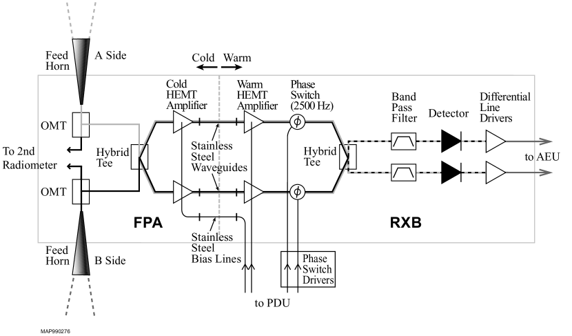
Figure 3: One half of a differencing assembly (DA) for detecting one polarization component. A hybrid Tee (“magic tee”) splits the inputs into two arms, where the signal is amplified and phase modulated before recombining. There are two stages of amplification, one at 90 K and one at 290 K. The recombined signal is then filtered and square law detected. The differential output that goes into the map-making algorithm is derived from the difference of the outputs of the two line drivers. From Jarosik et al. (2003a).

Figure 3 shows the signal path. From the output of the polarization selector (OMT), radiation from the two feeds is combined by a hybrid Tee into $(A+B)/\sqrt{2}$ and $(A-B)/\sqrt{2}$ signals, where A and B refer to the amplitudes of the electric fields from one linear polarization of each feed horn. In one arm of the receiver, both A and B signals are amplified first by cold ($90~{}$K) and then by warm (290 K) HEMT amplifiers. Noise power from the amplifiers, which far exceeds the input power, is added to each signal by the first amplifiers. Ignoring the phase switch for a moment, the two arms are then recombined in a second hybrid and both outputs of the hybrid are detected after a band-defining filter. Thus, for each differencing assembly, there are four detector outputs, two for each polarization. In a perfectly balanced system, one detector continuously measures the power in the A signal plus the average radiometer noise, while the other continuously measures the power in the B signal plus the average radiometer noise.

If the voltage amplification factors for the fields are $G_{1}$ and $G_{2}$ for the two arms, the difference in detector outputs is $G_{1}G_{2}(A^{2}-B^{2})$. Note that the average power signal present in both detectors has canceled so that small gain variations, which have a “$1/f$” spectrum, act on the difference in powers from the two arms, which corresponds to 0–3 K, rather than on the total power, which corresponds to roughly 100 K in the W band. The system is stabilized further by toggling one of the phase switches at 2.5 kHz and coherently demodulating the detector outputs. (The phase switch in the other arm is required to preserve the phase match between arms and is jammed in one state.) The 2.5 kHz modulation places the desired signal at a frequency above the $1/f$ knee of the detectors and audio amplifiers, as well as rejecting any residual effects due to $1/f$ fluctuations in the gain of the HEMT amplifiers. The power output of each detector is averaged for between 51 and 128 ms and telemetered to the Earth. In total, there are 40 signals (two for each radiometer) plus instrument housekeeping data, resulting in a data rate of 110 MBy/day.

It is difficult to overemphasize the importance of understanding the radiometer noise and the stability of the satellite. One of the requirements for producing high-quality maps is stable receivers. One aims to measure the largest and smallest angular scales before the instrument can drift. The main challenge is to design a system that is stable over the spin rate, when the largest angular scales are measured. The drift away from stability is generically termed “$1/f$”; the effects are similar to $1/f$ noise in amplifiers. The WMAP noise power spectrum is nearly white between 0.008 Hz, the spin rate of the satellite, and 2.5 kHz; however, there is a slight amount of $1/f$. With the exception of the W4 DA, the $1/f$ knee is below 9 mHz. For W4 it is 26 and 47 mHz for the two polarizations. To account for this the data are prewhitened in the map-making process. This is the primary correction made to the data and affects only the maps and not the power spectra, as discussed below.

Although WMAP’s differential design was driven by the $1/f$ noise in the amplifiers, it is also very effective at reducing the effects of $1/f$ thermal fluctuations of the spacecraft itself. The thermal stability of deep space combined with the insensitivity to the spacecraft’s slow temperature variations results in an extremely stable instrument. The measured peak-to-peak variation in the temperature of the cold end of the radiometers at the spin rate is $<12~{}\mu$K. Using the measured radiometer gain susceptibilities, this translates to a $<20~{}$nK radiometric signal. If one subtracts the sky signal from the data, the residual peak-to-peak radiometer output is measured to be $<0.17~{}\mu$K at the spin rate. Using the sky-subtracted signal, one can show that the receiver noise is Gaussian over 5 orders of magnitude (Jarosik et al. 2003). It is because of the stability, and our ability to verify it, that we can continuously average data together to probe cosmic signals at the sub-$\mu$K level.

3 Scan Strategy

High-quality maps are characterized by their fidelity to the true sky and their noise properties. Striping, the bane of the map-maker, results from scans of the sky in which the radiometer output departs from the average value for a significant part of the scan. Such departures, which can be produced by a number of mechanisms, are quantified as correlations between pixels.

A highly interlocking scan strategy is essential for producing a map with minimal striping. In any measurement, a baseline instrumental offset, along with its associated drift, must be subtracted. Without cross-hatched scans this subtraction can preferentially correlate pixels in large swaths, resulting in striped maps and substantially more involved analyses. WMAP’s noise matrix is nearly diagonal: the correlations between pixels are small. A typical off-diagonal element of the pixel-pixel covariance matrix is $<0.1$% the diagonal value, except in W4, where it is $\sim 0.5$% at small lag (Hinshaw et al. 2003a).

To achieve the interlocking scan, WMAP spins around its axis with a period of 2 min and precesses around a 22.^∘5 cone every hour so that the beams follow a spirograph pattern, as shown in Figure 4. Consequently, $\sim 30$% of the sky is covered in one hour, before the instrument temperature can change appreciably. The axis of this combined rotation/precession sweeps out approximately a great circle as the Earth orbits the Sun. In six months, the whole sky is mapped. The combination of WMAP’s four observing time scales (2.5 kHz, 2.1 min, 1 hour, 6 months) and the heavily interlocked pattern results in a strong spatial-temporal filter for any signal fixed in the sky.

Systematic effects at the spin period of the satellite are the most difficult to separate from true sky signal. Such effects, driven by the Sun, are minimized because the instrument is always in the shadow of the solar array and the precession axis is fixed with respect to the Sun-WMAP line. Spin-synchronous effects are negligible; there is no correction for them in the data processing.

With this scan, the instrument is continuously calibrated on the CMB dipole. The dominant signal in the timeline, the CMB dipole, averages to zero over the 1 hour precession period, enabling a clean separation between gain and baseline variations. The final absolute calibration is actually based on the component of the dipole due to the Earth’s velocity around the Sun. As a result, WMAP is calibrated to 0.5% (which will improve).

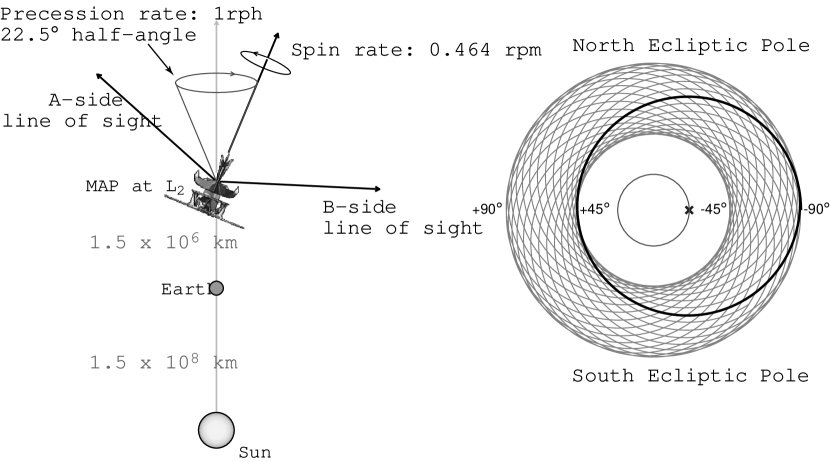
Figure 4: WMAP’s scan pattern from $L_{2}$. The dark circle on the left-hand drawing depicts the path covered by two beams for one rotation; the innermost circle is the path of the spin axis during one precession. The orbit follows a low-maintenance Lissajous pattern with the Sun, Earth, and Moon always behind. Corrections to the orbit are made roughly every three months. The scan motion is accomplished with three spinning momentum wheels so that the net angular momentum of the satellite is near zero. From Bennett et al. (2003a).

3 Basic Results

The primary scientific result from WMAP is a set of maps of the microwave sky of unprecedented precision and accuracy. The maps have a well-defined systematic error budget (Hinshaw et al. 2003a) and may be used to address the most basic cosmological questions, as well as to understand Galactic and extragalactic emission (Bennett et al. 2003).

The process of going from the differential radiometer data to the maps is described in Hinshaw et al. (2003a) and Wright, Hinshaw, & Bennett (1996). Each step of the process is checked with simulations that account for all known effects in the data stream.

There are many components of the map-making process that must be included to produce maps with minimal systematic error. They include masking bright sources when they are in one beam, deleting data around the 21 glitches, and solving for the baseline drift and gain. These effects would be part of any pipeline. In all, 99% of the raw data goes directly into the maps.

There are three systematic errors, all of which were anticipated, for which corrections are made. They are (1) the 4% sidelobe correction in K band that is applied directly to the K-band map, (2) the $\sim 1$% difference in loss between the A and B sides, and (3) the prewhitening described above. The last two are determined with flight data and are applied to the time stream. By any standards, this constitutes a remarkably little amount of correction. Artifacts from the gain, baseline, and pointing solutions are negligible.

Figures 5 and 6 show the maps in K through W bands. All maps have been smoothed to one degree. They are all in thermodynamic units relative to a 2.725 K blackbody, so that the CMB anisotropy has the same contrast in all maps. Emission from the Galactic plane saturates the color scale at all frequencies. At the lowest frequency, Galactic emission extends quite far off the plane. Still, even at 23 GHz, the anisotropy is clearly evident at high Galactic latitude. As one moves to higher frequency, there is less Galactic emission. When averaged over regions of high Galactic latitude, foreground contamination is minimum in V band.

There are a number checks that can be made of the maps. The simplest is shown in Figure 7. The sum of two channels of the same frequency gives a robust signal whereas the difference gives almost no signal. With the manifold instrumental redundancy, a myriad of other internal consistency checks is possible. We can also compare to the COBE/DMR map and see that, to within the limits of the noise, WMAP and DMR are the same. This is a wonderful confirmation of both satellites: they observe from different places, use different techniques, and have different systematic errors.

1 Analysis of Maps

The first step in going from the maps to cosmology is to select a region of sky for analysis. We mask regions that are significantly contaminated by diffuse emission from our Galaxy and by point source emission. Our selection process is described in Bennett et al. (2003c).

The diffuse contribution comes from free-free emission, synchrotron emission, and dust emission. To find the most contaminated sections, one masks regions that are above a threshold in the K-band maps. The nominal cut excludes 15% of the sky in a contiguous region near the Galactic plane.

One of the surprises from WMAP was that a successful model of the foregrounds could be made that did not include a spinning dust component (Draine & Lazarian 1998). Rather, we find that there is a strong correlation between synchrotron emission and dust, and that the synchrotron spectral index varies significantly over the Galactic plane. Surprising to many, the synchrotron emission is better correlated with the Finkbeiner, Davis, & Schlegel (1999) dust map derived from the COBE/DIRBE and IRAS at $\nu>200~{}$GHz than with the Haslam et al. (1982) synchrotron map at $\nu=0.41~{}$GHz.

In addition to diffuse emission, we mask a 0.^∘6 circle around 700 bright sources that might contaminate our results. The sources are selected based on radio catalogs, as discussed in Bennett et al. (2003c). No correlation with infrared sources was found. Contamination by point sources is a potential problem because their angular power spectrum has constant $C_{l}$, and thus rises as $l^{2}$ on the standard plot of the anisotropy. Our approach to identifying sources is three-pronged: (1) we search the data with a matched filter for sources, (2) we marginalize over a point source contribution in the determination of the angular power spectrum, and (3) we use a version of the bispectrum tuned to find point sources to directly

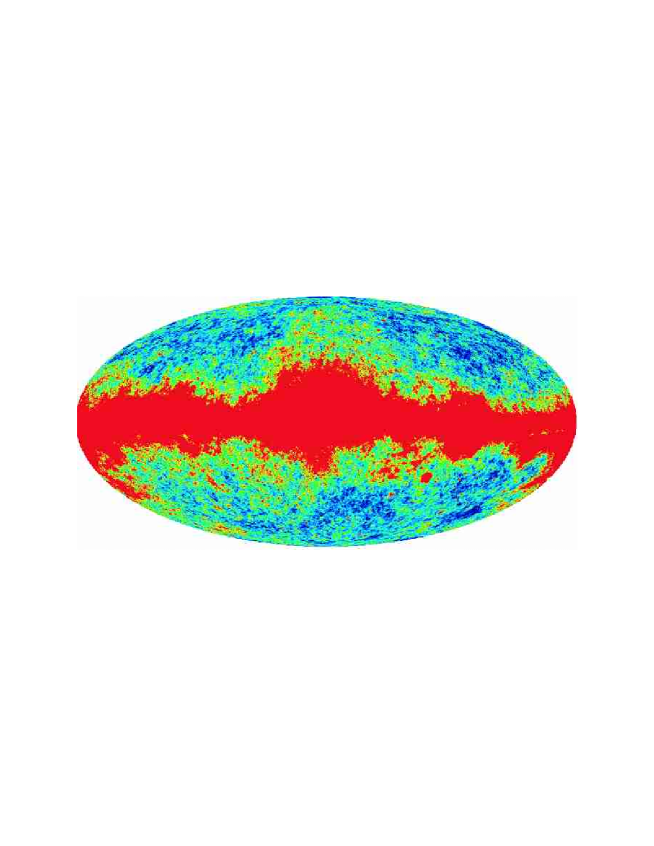
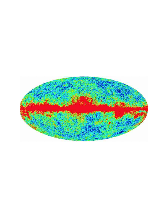
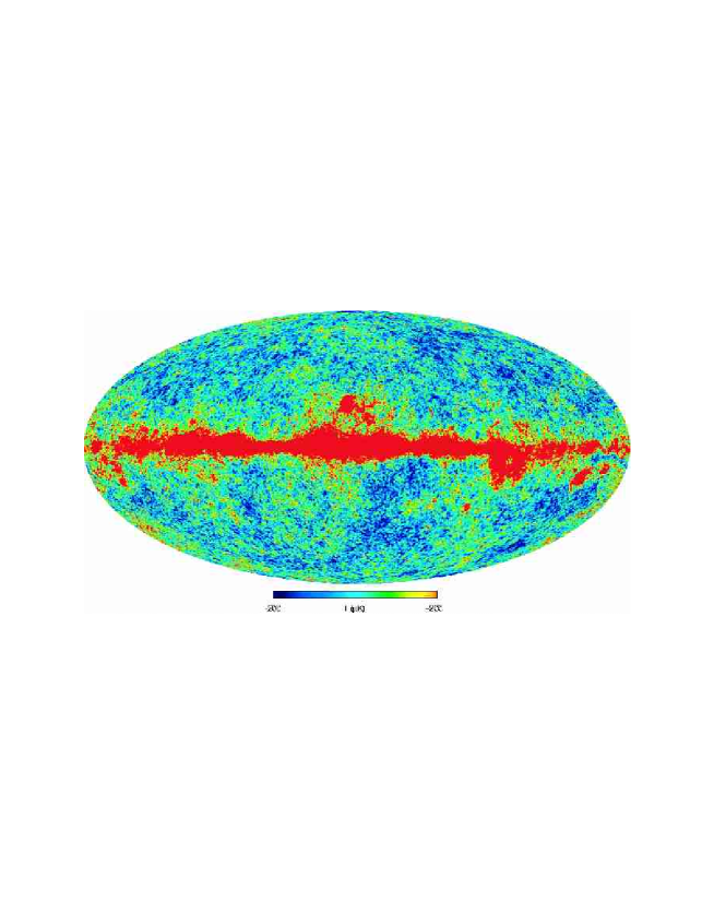
Figure 5: K-band (top), Ka-band (middle), and Q-band (bottom) intensity maps in Galactic coordinates shown in a Mollweide projection. The Galactic Center is in the middle of each map. All maps are in CMB thermodynamic units. From Bennett et al. (2003b).

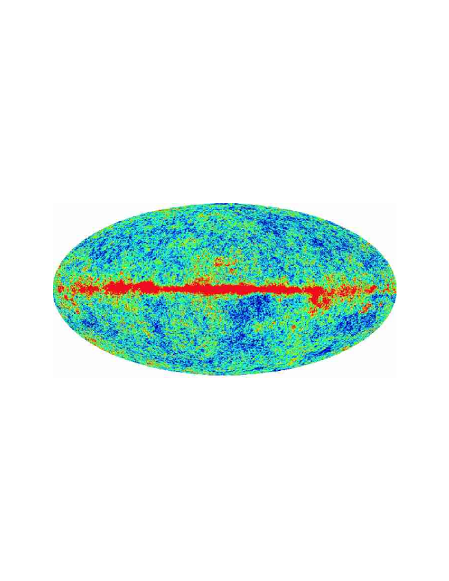
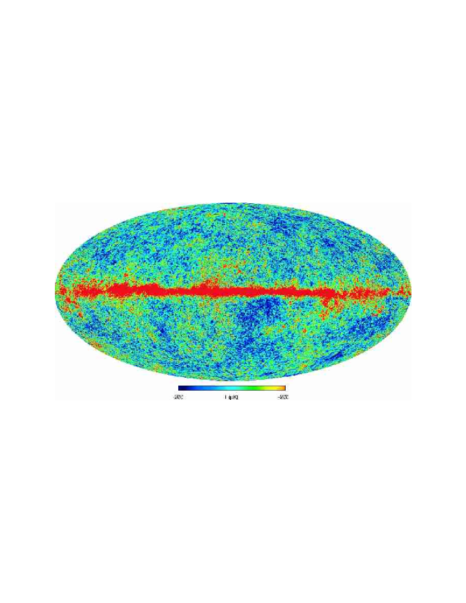
Figure 6: V-band (top) and W-band (bottom) maps in the same coordinates and scale as the previous three maps.

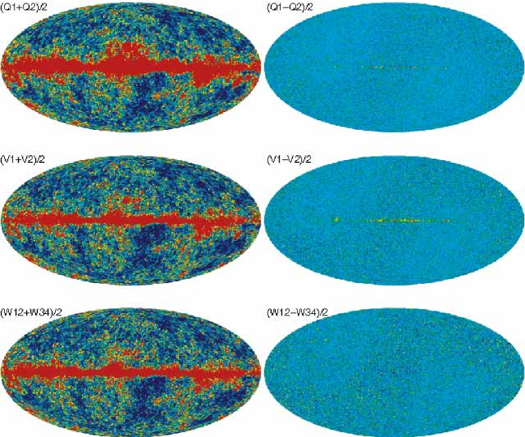
Figure 7: This plot shows the sum (left) and difference (right) maps for Q, V, and W, respectively. A slight bit of contamination is evident in V1–V2. This arises because the finite bandwidth of the passbands. The maps are calibrated with the CMB dipole, which has a different spectrum than the Galactic emission. In the bottom right panel especially, one can see that the noise in the maps is larger in the ecliptic plane. This is because the scan pattern preferentially samples the ecliptic poles. From Hinshaw et al. (2003b).

determine their contribution in a map. All three methods give consistent results when the sources are left in the map (Komatsu et al. 2003). All methods indicate that with our masking the sources do not contribute to the power spectrum.

After applying the diffuse and point source masks, the remaining parts of the maps are simultaneously fit to templates of the Finkbeiner et al. (1999) dust emission, an H$\alpha$ map that has been correct for extinction that traces free-free emission (see Finkbeiner 2003, and references therein), and a synchrotron map extrapolated from the 408 MHz Haslam et al. map.

The template fit removes any remaining residual Galaxy emission, even though the fit coefficients do not correspond to the best Galactic model. Tests are made to ensure that the masking and fitting do not bias the results.

With the maps in hand, we show that the fluctuations in the CMB are Gaussian to the level that can be probed with WMAP (Komatsu et al. 2003). This is a key step in the interpretation of the data. It means that all of the information in the CMB is contained in the angular power spectrum. In the parlance of CMB analyses, it means that if the temperature distribution is expanded in spherical harmonics as

$$T(\theta,\phi)=\sum_{lm}a_{lm}Y_{lm}(\theta,\phi),$$ (1)

that the real and the imaginary parts of the $a_{lm}$ are normally distributed. In other words, the phases between all the harmonics are random. There are no features in the CMB like strings or textures that require some definite relation between the phases. The Gaussanity of the CMB is a triumph for models such as inflation. However, the degree of non-Gaussanity expected from these models is a factor of 1000 or more below where WMAP can probe (Maldacena 2002).

From the masked and cleaned maps, we produce the angular power spectrum, as detailed in Hinshaw et al. (2003). All known effects are taken into account in going from the maps to the spectrum. We account for the uncertainty in the beam profile, foreground masking, and uneven weighting of the sky. Monte Carlo simulations are used to check that the noise is handled correctly. The stability of the instrument permits us to determine the noise contribution to the percent level. In producing the power spectrum we use only the cross correlations between the eight individual Q, V, and W intensity maps that have had the two polarizations combined (Hinshaw et al. 2003). Because the noise in the maps is, for all intents and purposes, independent, there are no effects from prewhitening or from the peculiarities of any one DA in the power spectrum. Of the possible 36 separate measures of the power spectrum, we use 28. The results are shown in the top panel of Figure 8.

We also produce maps of the Stokes $Q$ and $U$ polarization components (Hinshaw et al. 2003a; Kogut et al. 2003). These maps are produced from the difference of the two differential measurements common to one pair of feeds and use lines of constant Galactic longitude as a reference direction. Though the polarization maps pass a series of null tests, there was not enough time to prepare them for the first release. However, the cross correlation between the polarization and temperature maps is much less susceptible to systematic error than the polarization maps alone and may be more easily determined with confidence. At $>10\,\sigma$, we find a correlation between the Stokes $I$ (temperature) and $Q$ maps. This is due to the $E$ mode of the polarization (Kamionkowski, Kosowsky, & Stebbins 1997; Zaldarriaga & Seljak 1997). In Q, V, and W bands, the TE (Stokes $I$ cross $Q$) has a thermal frequency spectrum; it is not due to foregrounds. The correlation between Stokes $I$ and $U$, which is significant for $B$ modes, is consistent with zero.

The TE cross-power spectrum is shown in the bottom panel of Figure 8. We see that there is a model that describes the TT and TE data beautifully. As $E$ modes at $1^{\circ}$ scales are generated only during the transition from an ionized to a neutral Universe, the agreement indicates that we understand the physics of the decoupling process. Insofar as the $\ell>10$ TE correlation is predicted from the TT data, it does not contribute to our understanding of the cosmological parameters.

The TE correlation for $\ell<10$, however, considerably changes our understanding of cosmic history. It was a surprising discovery. The only way to polarize the CMB at these large angular scales is through reionization. In our fiducial model, we assume that the first generation of stars completely reionized the Universe at a fixed redshift, $z_{r}$. The optical depth, $\tau$, is then just the line integral out to $z_{r}$. We find that $\tau=0.17\pm 0.04$. Because quasar spectra show there is neutral hydrogen at $z=6$ (Becker et al. 2001; Djorgovski et al. 2001; Fan et al. 2002), the ionization history may not be as simple as in our model. After accounting for uncertainties in our model, we find $z_{r}=20^{+10}_{-9}$ (Kogut et al. 2003).

The large optical depth changes the way one interprets the TT power spectrum. It means that the intrinsic CMB fluctuations are 30% larger than the TT plot shows. This in turn affects the $\sigma_{8}$ (or overall normalization) one gets for the CMB data.

It is the maps and the power spectra that we derive from them that have the lasting value.

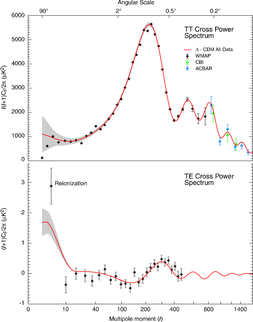
Figure 8: The top panel shows the net temperature-temperature (TT) cross-power spectrum between all channels. The measurement error bars are shown; the grey band shows the cosmic variance limit. WMAP is cosmic variance dominated up to roughly $\ell=350$. Below $\ell=100$, the noise is completely cosmic variance dominated and so we use only the V and W bands. For $\ell>700$ we augment WMAP with the data from CBI (Mason et al. 2003) and ACBAR (Kuo et al. 2003). The bottom panel shows the temperature-polarization (TE) cross-power spectrum. The point labeled “Reionization” is the weighted average of the lowest 8 multipoles. The red line is the best-fit model as discussed in §1. Note that the y-axis of the TE data is scaled to emphasize the low-$\ell$ region of the spectrum. (Hinshaw et al. 2003a)

Producing them is the primary goal of the mission. The maps do not depend on a particular cosmological model, the temperature power spectrum does not depend on a model, and the polarization does not depend on a model. We next focus more on to the cosmological interpretation of the data.

Figure 9: The contribution to the $\chi^{2}$ as a function of $\ell$. The spikes in this plot may be identified with departures from the best-fit model in Figure 8. The binning here is per $\ell$, whereas Figure 8 has values binned together. From Spergel et al. 2003.

2 Cosmic Parameters from Maps

One can deduce the parameters of the cosmological model that fit the data. The procedure is conceptually straightforward, though the devil is in the details. Advances have been made since the first estimates. One now uses numerically friendly combinations of parameters (e.g., Kosowsky, Milosavljević, & Jimenez 2002), customized versions of CMBFAST-like programs (Seljak & Zaldarriaga 1996), and Markov Chain Monte Carlos (Christensen et al. 2001).

For any model fitting, one assumes some prior information. For example, one might limit oneself to only adiabatic $\Lambda$CDM models, or, more restrictively, to models with $h>0.5$, or flat models, or models that agree with large-scale structure data. A goal is to say as much as possible with the minimum number of priors.

For the simplest models of the CMB, there is an intrinsic parameter degeneracy called the “geometric degeneracy” (Bond et al. 1994; Zaldarriaga, Spergel, & Seljak 1997). Using the TT CMB data alone, one cannot separately determine $\Omega_{m}$, $h$, and $\Omega_{\Lambda}$ even with cosmic variance limited data out to $\ell=2000$. One can play these parameters off one another to produce identical spectra. The degeneracy is broken by picking a value of the Hubble constant, assuming a flat geometry, or something similar. With the WMAP data, supernovae data (Riess et al. 1998; Perlmutter et al. 1999), and the HST Key Project value of $h=0.72\pm 3\pm 7$ (Freedman et al. 2001), $\Omega_{T}=1.02\pm 0.02$. With the WMAP data and a prior of $h>0.5$, $0.98<\Omega_{T}<1.08$ (95% confidence). While this does not prove that the Universe is geometrically flat, Occam’s razor and the Dicke arguments that in part inspired inflation lead one to take a flat Universe as the basic model.

Unless otherwise noted, all the parameters quoted have a prior that the Universe is geometrically flat. With this, the values in Table 2 are obtained. We give the values for just power-law models for the index. Values for a variety of models and parameter combinations are given in Spergel et al. (2003).

Table 2: Sample of Best-Fit Cosmological Parameters

Parameter		WMAP only, flat	WMAP+others	Non-CMB estimates
$A$		$0.9\pm 0.1$	$0.75^{+0.08}_{-0.07}$	…
$\tau$		$0.166^{+0.076}_{-0.071}$	$0.117^{+0.057}_{-0.053}$	…
$\Omega_{b}h^{2}$		$0.024\pm 0.001$	$0.0226\pm 0.0008$	$0.021-0.025$
$\Omega_{m}h^{2}$		$0.14\pm 0.02$	$0.133\pm 0.006$	$0.062-0.18$
$h$		$0.72\pm 0.05$	$0.72\pm 0.03$	$h=0.72\pm 3\pm 7$
$n_{s}$		$0.99\pm 0.04$	$0.96\pm 0.02$	…
$\chi^{2}_{eff}/\nu$		$1431/1342=1.066$	…	…

The best-fit parameters for the WMAP data for two of the models tested. The second column is for WMAP alone; the third is for a combination of WMAP+CBI+ACBAR+2dFGRS+Ly$\alpha$. The $\chi^{2}$ is not given because the Ly$\alpha$ data are correlated. The non-CMB estimates are from studies of the Ly$\alpha$ D/H and DLA systems, cluster number counts, galaxy velocities, and the HST Key Project. They come from many studies and are discussed in Spergel et al. (2003).

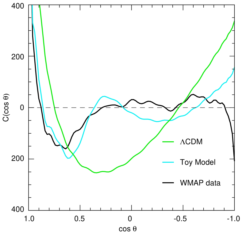
Figure 10: Correlation function of the WMAP data. The green line corresponds to a $\Lambda$CDM model. The black line is the WMAP data. The “Toy” model, described in Spergel et al. (2003), has been tailored to fit the data by putting discrete modes in the matter power spectrum.

It is of interest that the reduced $\chi^{2}$ for the best-fit model has a probability to exceed of $\sim 5$%. The reduced $\chi^{2}$ is slightly large, but on its own does not signal that the model is wrong. In fact, no matter what model we try, $\chi^{2}/\nu$ more or less stays the same. If isocurvature modes are added to fit the low-$\ell$ region of the spectrum, $\chi^{2}/\nu=1468/1378=1.065$ (Peiris et al.  2003); if one adds tensor modes, allows the spectral index $n_{s}$ to run, and the 2dFRGS data are added, $\chi^{2}/\nu=1465/1379=1.062$; if a step is added to the power spectrum that attempts to fit bumps and wiggles in the WMAP angular power spectrum, $\chi^{2}/\nu=1422/1339=1.062$ (Peiris et al.  2003). In other words, the admixture of additional model elements does not substantially improve the fit over the basic model. The contributions to $\chi^{2}/\nu$ are shown in Figure 9. It is likely that, as the sky is covered more thoroughly, as we understand the beams better, and as we account for more detailed astrophysical effects (Spergel et al.  2003), $\chi^{2}$ will decrease.

Though the simple model is a wonderful fit to the WMAP data, the small quadrupole and the related lack of correlation at large angular separations is striking. Though largely obscured by cosmic variance, there appears not even a hint of an upturn at low $\ell$, as expected in $\Lambda$CDM models. (However, COBE also found no evidence for such an upturn). This departure from the model constitutes a small (though possibly important) fraction of the total fluctuation power and does not cast doubt on the interpretation of the $\ell>40$ spectrum. The correlation function is shown in Figure 10. For $\theta>60^{\circ}$ the probability that the WMAP data agree with the best-fit $\Lambda$CDM models at these angular scales is $\sim 1/500$. One must keep in mind that the statistic is a posteriori, but it is still unsettling.

4 Summary and the Future

Before it was widely appreciated that so many of the cosmological parameters could be deduced directly from the CMB (e.g., Jungman et al. 1995), the motivation for studying the anisotropy was that it would tell us the initial conditions for the formation of cosmic structure and would tell us the cosmogony in which to interpret that process. In this vein, we summarize here some of the grander conclusions we have learned from WMAP.

1. A flat $\Lambda$-dominated CDM model with just six parameters ($A$, $\tau$, $\Omega_{m}$, $\Omega_{b}$, $h$, and $n_{s}$) gives an excellent description of the statistical properties of $>10^{6}$ measurements of the anisotropy over 85% of the sky. This does not mean that a simple flat $\Lambda$CDM model is complete, but any other model must look very much like it.

2. An Einstein-de Sitter model, which is flat with $\Omega_{\Lambda}=0$, is ruled out at $>5\,\sigma$. This statement is based on just the CMB, with no prior information (e.g., no prior on $h$). Stated another way, if $h>0.5$ then WMAP requires $\Omega_{\Lambda}\neq 0$ in the angular-diameter distance to the decoupling surface.

3. A closed model with $\Omega_{m}=1.28$ and $\Omega_{\Lambda}=0$ fits the data but requires $h=0.33$, in conflict with HST observations. It also disagrees with cluster abundances, velocity flows, and other cosmic probes.

4. The fluctuations in the metric are superhorizon (Peiris et al. 2003). Turok (1996) showed that in principle one can construct models based on subhorizon processes that can mimic the TT $\Lambda$CDM spectra. However, these models cannot mimic the observed TE anticorrelation at $50<\ell<150$ (Spergel & Zaldarriaga 1997).

By combining WMAP data with other probes we can constrain the mass of the neutrino and constrain the equation of state, $w$. As our knowledge of the large-scale structure matures, in particular of the Ly$\alpha$ forest (McDonald et al.  2000; Zaldarriaga, Hui, & Tegmark 2001; Croft et al.  2002; Gnedin& Hamilton  2002; Seljak, McDonald, & Markarov 2003), we can use the combination of these measurements to probe in detail the spectral index as a function of scale, thereby directly constraining inflation and other related models. No doubt correlations with other measurements will shed light on other cosmic phenomena. With WMAP, physical cosmology has moved from assuming a model and deducing cosmic parameters to detailed testing of a standard model.

The WMAP mission is currently funded to run through October 2005, though as of this writing there is nothing to limit the satellite from operating longer. The quality of the maps will continue to improve as the mission progresses. Not only will the noise integrate down, but our knowledge of the beams will continue to improve, and we will make corrections that were too small to consider for the year one analysis. For example, increased knowledge of the beams will reduce the uncertainties in the power spectrum at high $\ell$ and will permit an even cleaner separation of the CMB and foreground components near the Galactic plane. It is the set of high-fidelity maps of the microwave sky that will be WMAP’s most important legacy.

With four-year maps, the polarization at intermediate and large angular scale should be seen and the epoch of reionization will be much better constrained. It may even be possible to detect the lensing of the CMB by the intervening mass fluctuations.

On the horizon is the Planck satellite, which, with its higher sensitivity, greater resolution, and larger frequency range should, significantly expand upon the picture presented by WMAP. In addition, a host of other measurements that push to yet finer angular scales and a future satellite dedicated to measuring the polarization in the CMB, especially the $B$ modes, promise a rich and exciting future for CMB studies.

More information about WMAP and the data are available through:
http://lambda.gsfc.nasa.gov/

References

- [1] Barnes, C., et al. 2002, ApJS, 143, 567
- [2] ——. 2003, ApJ, submitted (astro-ph/0302215)
- [3] Becker, R. H., et al. 2001, AJ, 122, 2850
- [4] Bennett, C. L., et al. 2003a, ApJ, 583, 1
- [5] ——. 2003b, ApJ, submitted (astro-ph/0302207)
- [6] ——. 2003c, ApJ, submitted (astro-ph/0302208)
- [7] Bond, J. R., Crittenden, R., Davis, R. L., Efstathiou, G., & Steinhardt, P. J. 1994, Phys. Rev. Lett., 72, 13
- [8] Christensen, N., Meyer, R., Knox, L., & Luey, B. 2001, Classical and Quantum Gravity, 18, 2677
- [9] Colless, M., et al. 2001, MNRAS, 328, 1039
- [10] Croft, R. A. C., Weinberg, D. H., Bolte, M., Burles, S., Hernquist, L., Katz, N., Kirkman, D., & Tytler, D. 2002, ApJ, 581, 20
- [11] Djorgovski, S. G., Castro, S., Stern, D., & Mahabal, A. A. 2001, ApJ, 560, L5
- [12] Draine, B. T., & Lazarian, A. 1998, ApJ, 494, L19
- [13] Fan, X., et al. 2002, AJ, 123, 1247
- [14] Finkbeiner, D. P. 2003, ApJS, 146, 407
- [15] Finkbeiner, D. P., Davis, M., & Schlegel, D. J. 1999, ApJ, 524, 867
- [16] Freedman, W. L., et al. 2001, ApJ, 553, 47
- [17] Gnedin, N. Y., & Hamilton, A. J. S. 2002 MNRAS, 334, 107
- [18] Haslam, C. G. T., Stoffel, H., Salter, C. J., & Wilson, W. E. 1982, A&AS, 47, 1
- [19] Hinshaw, G., et al. 2003a, ApJ, submitted (astro-ph/0302222)
- [20] ——. 2003b, ApJ, submitted (astro-ph/0302217)
- [21] Jarosik, N., et al. 2003a, ApJS, 145, 413
- [22] ——. 2003b, ApJ, submitted (astro-ph/0302224)
- [23] Jungman, G., Kamionkowski, M., Kosowsky, A., & Spergel, D. N. 1995, Phys. Rev. D., 54, 1332
- [24] Kamionkowski, M., Kosowsky, A., & Stebbins, A. 1997, Phys. Rev. D, 55, 7368
- [25] Kamionkowski, M., Spergel, D. N., & Sugiyama, N. 1994, ApJ, 426, L57
- [26] Kogut, A., et al. 2003, ApJ, submitted (astro-ph/0302213)
- [27] Komatsu, E., et al. 2003, ApJ, submitted (astro-ph/0302223)
- [28] Kosowsky, A., Milosavljević, M., & Jimenez, R. 2002, Phys. Rev. D, 66, 63007
- [29] Kuo, C. L., et al. 2003, ApJ, submitted (astro-ph/0212289)
- [30] Maldacena, J. 2002, preprint (astro-ph/0210603)
- [31] Mason, B. S., et al. 2003, ApJ, in press (astro-ph/0205384)
- [32] McDonald, P., Miralda-Escudé, J., Rauch, M., Sargent, W. L. W., Barlow, T. A., Cen, R., & Ostriker, J. P. 2000, ApJ, 543, 1
- [33] Page, L. A., et al. 2003a, ApJ, 585, 566
- [34] ——. 2003b, ApJ, submitted (astro-ph/0302214)
- [35] ——. 2003c, ApJ, submitted (astro-ph/0302220)
- [36] Peiris, H., et al. 2003, ApJ, submitted (astro-ph/0302225)
- [37] Perlmutter, S., et al. 1999, ApJ, 517, 565
- [38] Pospieszalski, M. W. 1992, Proc. IEEE Microwave Theory Tech., MTT-S 1369
- [39] ——. 1997, Microwave Background Anisotropies, ed. F. R. Bouchet (Gif-sur-Yvette: Editions Frontièrs), 23
- [40] Pospieszalski, M. W., & Wollack, E. W. 1998, IEEE Microwave Theory Tech., MTT-S Digest, Baltimore, MD 669
- [41] Riess, A. G., et al. 1998, AJ, 116, 1009
- [42] Seljak, U., McDonald, P., & Markarov, A. 2003, MNRAS, in press (astro-ph/0302571)
- [43] Seljak, U., & Zaldarriaga, M. 1996, ApJ, 469, 437
- [44] Spergel, D. N., et al. 2003, ApJ, submitted (astro-ph/0302209)
- [45] Spergel, D. N., & Zaldarriaga, M. 1997, Phys. Rev. Lett., 79, 2180
- [46] Turok, N. 1996, Phys. Rev. D, 54, 3686
- [47] Verde, L., et al. 2003, ApJ, submitted (astro-ph/0302218)
- [48] Wright, E. L., Hinshaw, G., & Bennett, C. L. 1996, ApJ, 458, L53
- [49] Zaldarriaga, M., Hui, L., & Tegmark, M. 2001, ApJ, 557, 519
- [50] Zaldarriaga, M., & Seljak, U. 1997, Phys. Rev. D, 55, 1830
- [51] Zaldarriaga, M., Spergel, D. N., & Seljak, U. 1997, ApJ, 488, 1