The Coronae of AR Lac
Abstract
We observed the coronally active eclipsing binary AR Lac with the High Energy Transmission Grating on Chandra for a total of 97 ks, spaced over five orbits, at quadratures and conjunctions. Contemporaneous and simultaneous EUV spectra and photometry were also obtained with the Extreme Ultraviolet Explorer. Significant variability in both X-ray and EUV fluxes were observed, dominated by at least one X-ray flare and one EUV flare. We saw no evidence of primary or secondary eclipses, but exposures at these phases were short and intrinsic variability compromised detection of any geometric modulation. X-ray flux modulation was largest at high temperature, indicative of flare heating of coronal plasma rather than changes in emitting volume or global emission measure. Analysis of spectral line widths interpreted in terms of Doppler broadening suggests that both binary stellar components are active. Based on line fluxes obtained from total integrated spectra, we have modeled the emission measure and abundance distributions. The EUV spectral line fluxes were particularly useful for constraining the parameters of the “cool” ( K) plasma. A strong maximum was found in the differential emission measure, characterized by two apparent peaks at and , together with a weak but significant cooler maximum near , and a moderately strong hot tail from . Coronal abundances have a broad distribution and show no simple correlation with first ionization potential. While the resulting model spectrum generally agrees very well with the observed spectrum, there are some significant discrepancies, especially among the many Fe L-lines. Both the emission measure and abundance distributions are qualitatively similar to prior determinations from other X-ray and ultraviolet spectra, indicating some long-term stability in the overall coronal structure.
1 Introduction
AR Lac (HD 210334, HR 8448) is one of the brightest totally eclipsing RS CVn binaries. Since eclipses can help constrain active region geometry, it has been a key system for studying the structure of photospheric spots from visible light modulation, the chromosphere from emission of magnesium, calcium and hydrogen, the transition region through ultraviolet emission lines, and the coronae via emission at extreme ultraviolet (EUV), X-ray, and radio wavelengths. There is as yet no comprehensive predictive theory that explains in detail all the aspects of coronal emission based only on fundamental stellar parameters. Observational attack is then aimed at increasing the quantity and quality of spectral and photometric data to provide insights and to help constrain the dependence of coronal activity on stellar evolutionary parameters, other magnetic activity indicators or as yet unidentified parameters. With the High Energy Transmission Grating Spectrometer (HETGS) on the Chandra X-Ray Observatory, we are able to greatly improve the quality of X-ray spectra by resolving a multitude of coronal emission lines due to iron and the hydrogen-like and helium-like lines of a number of abundant elements. These spectra provide both line and continuum fluxes and their time variability. The aim of this study is to model the lines and continuum with the latest atomic data in order to determine the coronal temperature structure, density and absolute elemental abundances.
AR Lac is comprised of G- and K-type subgiants in a 1.98 day orbit. The components are each of slightly greater than one Solar mass ( and , respectively) and have radii of and . They reach a maximum radial velocity separation of and have rotational velocities of 39 and 70 . At a distance of 42 pc, AR Lac is relatively bright. Gehren, Ottmann & Reetz (1999) summarized these and other fundamental properties of AR Lac.
AR Lac was detected in X-rays by HEAO 1 at a luminosity of (Walter et al., 1980); Walter, Gibson & Basri (1983) present an early analysis of the X-ray coronae in which it was inferred that emission arose from both stellar components in compact and extended structures. Subsequent X-ray studies were undertaken by Ottmann, Schmitt & Kuerster (1993) (ROSAT), White et al. (1990) (EXOSAT), Rodonò et al. (1999) (Beppo-SAX), and White et al. (1994) (ASCA).
Observations with ROSAT and ASCA detected a deep primary eclipse and a smaller secondary eclipse (Ottmann & Schmitt, 1994; White et al., 1994), while EXOSAT and EUVE observations could only confirm the primary eclipse due to flares or instrumental limitations (White et al., 1990; Christian et al., 1996; Brickhouse et al., 1999; Pease et al., 2002). Some extended chromospheric material was also detected by Montes et al. (1997) and Frasca et al. (2000). Analysis of high resolution EUVE data (Griffiths & Jordan, 1998; Brickhouse et al., 1999; Sanz-Forcada, Brickhouse & Dupree, 2003) showed a corona dominated by material at K, and a substantial amount of material at hotter temperatures of K.
2 Observations and Data Processing
2.1 Chandra/HETGS
We observed AR Lac six times (observation identifiers (OID), 6–11) with the Chandra X-Ray Observatory’s HETG/ACIS-S instrument (HETGS) (Weisskopf et al., 2002) in standard timed-event mode. Two longer exposures (35 ks) were at the same orbital quadrature. Four shorter observations ( ks) were paired at the two eclipses.111Caveat: due to an 0.5 day ephemeris error, comments on the phase in the standard data product headers are wrong. In an attempt to minimize uncertainties from any long term trends in activity, all the data were taken within five orbits of this two day period binary. We applied the ephemeris of Perryman et al. (1997), which differs from the more recent determination by Marino et al. (1998) by less than 0.01 in phase at the epoch of observation. Observational details are given in Table 1.
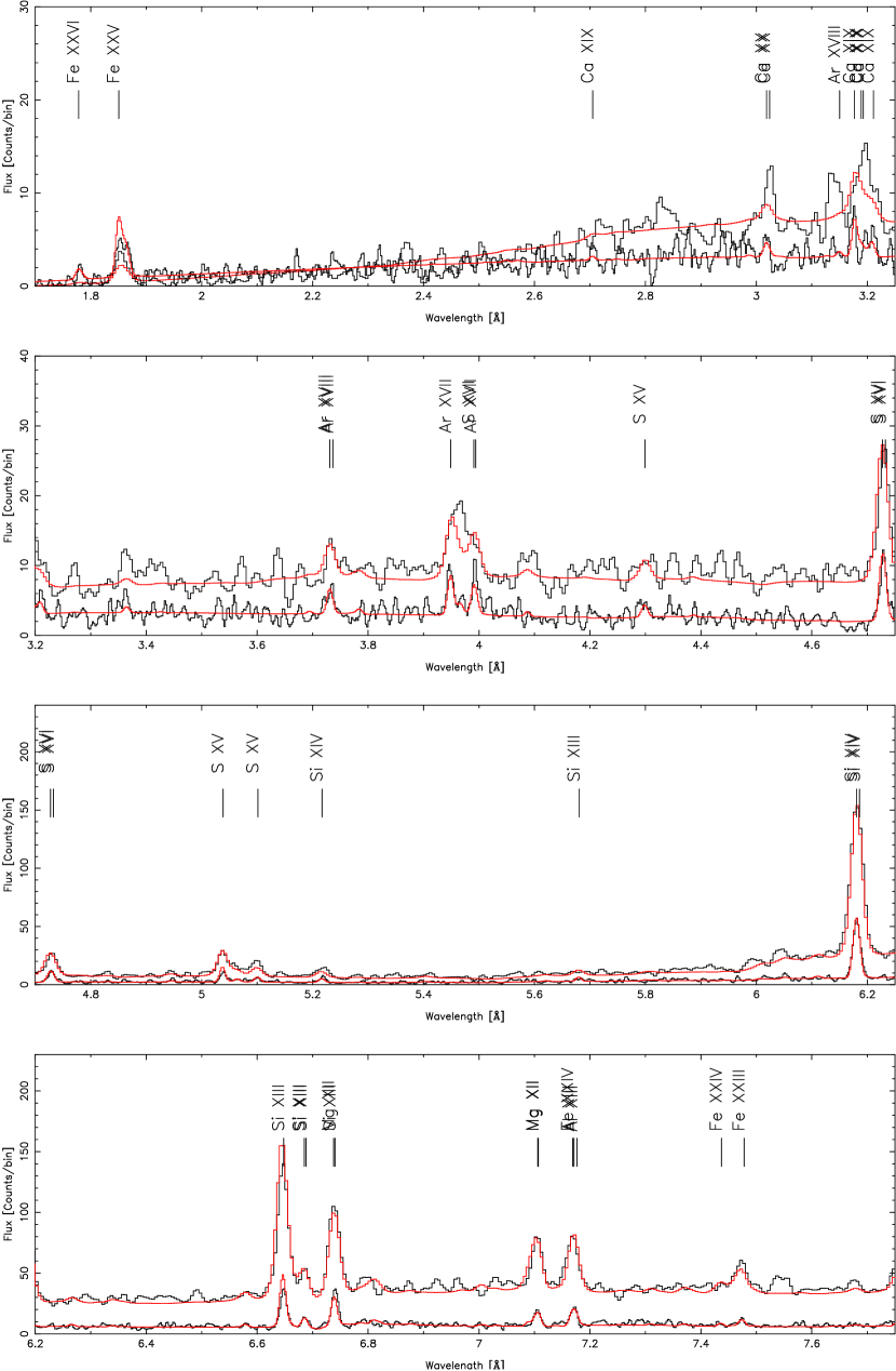
The event files were re-processed to apply updated calibration files (namely, CCD gain and bad-pixel filters; we used ASCDSVER CIAO 2.1 Wednesday, February 28, 2001 and CALDBVER 2.3). Data were also “de-streaked” to filter out the instrumental artifact on CCD-8 and then processed to grating coordinates. These event lists were then binned onto the standard CIAO222http:cxc.harvard.edu HETGS spectral grids. Effective area tables (auxiliary response files, or ARFs) were made with CIAO software (mkgarf) for each of the HEG and MEG gratings, and for and orders. We show a summary flux spectrum in Figure 1.
2.2 EUVE
EUVE spectrographs cover the spectral range 70–180 Å, 170–370 Å and 300–750 Å for the short-wavelength (SW), medium-wavelength (MW) and long-wavelength (LW) spectrometers respectively, with corresponding spectral dispersion of , , and Å/pixel, and an effective spectral resolution of –. The Deep (DS) Survey Imager has a band pass of 80–180 Å (Haisch, Bowyer & Malina, 1993). Standard data products from the EUVE observations of AR Lac were obtained through the Multimission Archive at Space Telescope (MAST), corresponding to three observational campaigns starting in 1993 October 12 (96 ks), 1997 July 3 (74 ks) and 2000 September 14 (63 ks).
3 Photometric Analysis
3.1 Lightcurves
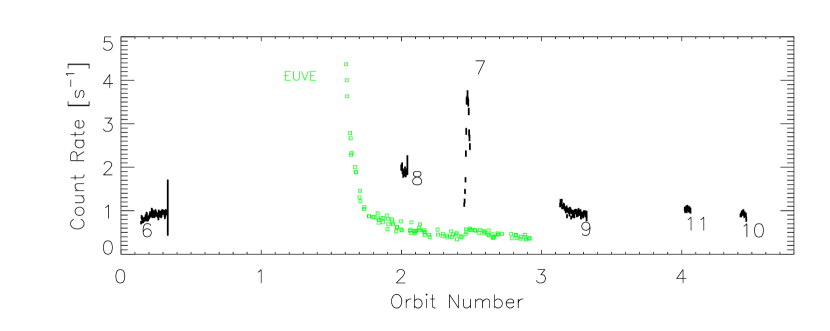
We made light curves of the Chandra data using the CIAO program lightcurve, and filtered the input events so that to orders (excluding zero, which is piled333“Pileup” refers to coincidence of photons in the same spatial and temporal bins. It makes the response non-linear, and also, if severe, censors counts via on-board filtering.), and MEG and HEG photons within 1–25 Å were all binned into one curve for each OID. We also made light curves in some stronger line and continuum bands by filtering on narrow wavelength regions. We show some of the light curves in Figure 2.
EUVE light curves (small open squares in Figure 2) were built from the DS image by taking a circle centered on the source, and subtracting the sky background within an annulus around the center. Standard procedures were used in the IRAF package EUV v. 1.9, with a time binning of 600 s. In the following discussion and analysis, the observations in 1993 and 1997 are referred to as “quiescent” states; despite of the presence of some minor flares the apparently quiescent component dominates the integrated flux (Sanz-Forcada, Brickhouse & Dupree, 2003). The observations in 2000 are instead referred to as a “flare” state. Only the observations of the 2000 campaign, contemporaneous with the Chandra observations, are employed here.
3.2 Variability
From the X-ray light curve in Figure 2 we see that AR Lac was highly variable during the observations. There is one obvious flare near phase 0.5 (orbit 2.5, OID 7) when the count rate increased by nearly a factor of four, and then rapidly decayed. A little more than half an orbit later (orbit 3, phase 0.13-0.33, OID 9), the count rate was decreasing. It is tempting to associate this with the tail of the larger flare, but it could just as well be an independent event. For the two consecutive segments to connect smoothly, the decay rate would have to be variable in a complicated way; the estimated decay rate of OID 9 is too short to connect with the previous flare. Given that OID 8 is somewhat elevated in count rate and fairly steady, this would be consistent with the high flare frequency and broad range of decay rates that AR Lac typically exhibits, as revealed by the extensive EUVE and Chandra lightcurves analysed by Pease et al. (2002).
We can use the EUVE light curve (Figure 2) to provide a context for the disjoint X-ray observations. The Chandra OID 7 flare was simultaneously observed with the EUVE, which showed a small step up in count rate. A large EUV flare occurred between OID 6 and 8. Assuming that the high X-ray to EUV enhancement ratio seen in OID 7 always holds, which would be more indicative of further heating of an existing volume of hot plasma rather than evaporation of cold chromospheric material, the EUV flare must have started after OID 6. The baseline trend from OID 8-7-9 is probably indicative of the decay of the large flare. There is no obvious quiescent state; the nearest hint of one is from phase 0.25-0.30. One observation (OID 9) is decreasing to this level, but the other (OID 6) is actually increasing from a lower flux state.
There are no obvious X-ray eclipses, but exposures were short at these phases. The dotted curve in Figure 2 is a simple occultation model with uniform disks of equal surface brightness and with relative radii in proportion to the AR Lac components, scaled arbitrarily. The lower X-ray flux state during primary eclipse egress (OID 11; phase 0.0-0.1) is constant. This implies that the emerging, smaller G-star is X-ray dark, is dark on the portion being exposed, or that emission structures are large and polar so they are not occulted. We will rule out the former case later, based on line-profile information (see 4.4).
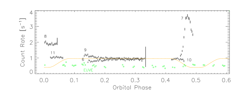
To investigate qualitative temperature changes, we binned light curves in narrow bands, for both continuum and strong line regions. Continuua near lines were used to derive net line rates, and some features with similar temperatures of maximum emissivity were summed to improve statistics. An example is shown in Figure 2 for Si xiv (6.18 Å, ), which follows the overall integrated light curve, and Si xiii (6.6-6.8 Å, ), whose net rate shows little variation. As a qualitative temperature diagnostic, we computed the modulation in the count rate, , for each feature, defined as , which is 1.0 for maximum modulation (, to 0.0 for constant count rate (). In Figure 3 we show the modulation as a function of temperature of formation. For lines, the temperature of formation is defined as the temperature of maximum emissivity.
The trend in modulation is clear from these light curves: higher temperature emission is more modulated. The cutoff is quite sharp for the lines at about . The ion temperature, though, is not a unique diagnostic. For example, the difference in modulation between Mg xii and Si xiii is not contradictory, since Mg xii is hydrogen-like and has a long emissivity tail extending to higher temperatures. The continuum modulation showed a similar trend, in that the continuum flux at shorter wavelengths, which is formed by higher temperature plasma, is also more strongly modulated.
As another qualitative diagnostic of temperature changes, we looked at band light curve ratios to see if the decrease in OID 9 is a flare decay (after the EUVE observation, on the extreme tail of the EUV flare), and whether the slight rise in OID 6 in the same phase interval (but before the EUV flare) could be due to rotational modulation of asymmetrically distributed X-ray emitting structures. We used the strongly modulated 1.9-2.9 Å band light curve for the high temperature diagnostic, the relatively unmodulated Fe xvii regions’ continuum bands (14.7-14.9, 16.4-16.6, and 17.2-17.5 Å) as well as Ne x to sample the cooler plasma. The ratios clearly showed the flares near phases 0 and 0.5, but no significant differences at the quadrature phases. We cannot say whether either the slow rise or fall are due to flares or rotational modulation. But given the large EUV flare, the OID 9 decrease is probably due to flare decay, and temperature changes are below the sensitivity of the observations.
4 Spectroscopic Analysis
4.1 Spectral Line Fluxes
4.1.1 Chandra Spectra
Obtaining line fluxes from coronal X-ray spectra such as that of AR Lac is complicated by the presence of continuum flux. This continuum has a shape which is dependent primarily on the plasma temperature. In order to extract line fluxes, we therefore adopted an iterative approach, whereby temperature information from spectral lines was used to calculate a model continuum, which was then used to refine measurements of the line fluxes.
We summed orders and fit line fluxes with the CXC software suite, ISIS (Houck & Denicola, 2000).444http://space.mit.edu/CXC/ISIS Emission lines were fit by convolving intrinsic source line profiles (Gaussians) plus a model plasma continuum by the instrumental response or line spread function (LSF). The free parameters were the Gaussian centroids and areas of each line, and, if necessary, the Gaussian dispersion. Typically, the lines are unresolved, so the Gaussian dispersion was frozen at a value well below the instrumental resolution. For some cases, either due to blends or to orbital velocity separation, we fit the line width (line widths are discussed in 4.4). The redistribution component of the response for grating spectra is the line spread function (LSF), which is stored in grating redistribution matrix files (RMF) in the CIAO calibration database. HEG and MEG spectra were kept separate, but fit simultaneously. The continuum model was obtained iteratively, first by fitting relatively line-free regions with a single temperature plasma model, and subsequently by using the result of differential emission measure models to improve the predicted continuum. The continuum normalization was not allowed to vary in the fitting since the apparent continuum is often significantly above the true continuum due to line blending. For the continuum model, we use the summed true continuum and pseudo-continuum components in the Astrophysical Plasma Emission Database (APED; Smith et al., 2001).
To be explicit, if the model line contribution, , to a region is expressed as a sum of normalized Gaussians, , enumerated by component , as
| (1) |
then the iteration predicted counts spectrum in the region of interest can be defined as
| (2) |
Here, is the detected channel, the wavelength, the continuum source model, the redistribution function (LSF; or response matrix, RMF), and the effective area. The values are the line fluxes, and and are the line centroid and dispersion, respectively. The line fluxes determined by minimizing this against the counts are listed in Table 2.
4.1.2 EUVE Spectra
Spectra of AR Lac, binned over the total observation, were used to provide fluxes of lines in the range 90–400 Å as listed in Table 2. To correct the observed fluxes for interstellar hydrogen and helium continuum absorption, we used a ratio He i/H i=0.09 (Kimble et al., 1993), and a value of , calculated from the Fe xvi line ratio. Lines of Fe ix–Fe xxiv (except Fe xvii) are formed in this spectral range, providing good coverage in temperature from only one element over the range K, avoiding the introduction of further uncertainties from the calculation of abundances.
4.2 Temperature Distribution
A more quantitative description of plasma temperatures is given by the emission measure distribution. This is a one-dimensional characterization of an emitting plasma describing the emitting power as a function of temperature. It does not tell us how the material is arranged geometrically. This must be derived from other information, such as eclipse or rotational modulation, or inferred through (hopefully realistic) assumptions of parametric or semi-empirical models such as hydrostatic, magnetically confined loops. Nonetheless, the emission measure distribution remains a useful quantity for visualization and comparative study of coronal temperature structure. Bowyer, Drake & Vennes (2000) present a good review of emission measure modeling in the context of cool stars and extreme ultraviolet spectroscopy.
There are many pitfalls in inverting the emission integral (Craig & Brown, 1976; Hubeny & Judge, 1995; McIntosh, Brown & Judge, 1998; Judge, Hubeny & Brown, 1997). Inversion is limited by the emissivity functions of real atoms, which do not form an orthogonal set of basis functions; some kind of regularization is necessary. Kashyap & Drake (1998) also discuss problems of spurious structure caused by errors in atomic data, and describe an approach to the problem based on a monte carlo technique converged by a Markov chain which includes atomic data as well as line measurement uncertainties.
In this analysis, we fit the differential emission measure (DEM) and abundances simultaneously by minimizing the integrated line flux residuals using the emissivities from the APED and the ionization balance of Mazzotta et al. (1998). Our basic method is described by Huenemoerder, Canizares & Schulz (2001). We minimize a statistic,
| (3) |
Here, is a spectral feature index, and is the temperature index. The measured quantities are the line fluxes, , with uncertainties . The a priori given information are the emissivities, , and the source distance, . The minimization provides a solution for the differential emission measure, and abundances of elements , . The exponentiation of is simply a trick which forces to be non-negative, and is a smoothing operator which imposes some implicit regularization on the solution; we use a Gaussian convolution with a dispersion of 0.15 dex. We omit spectral features which are line blends of different elements and of comparable strengths. We use a temperature grid of 60 points spaced by 0.05 in , from to 8.5. The emissivities, , are as defined by Raymond & Brickhouse (1996). We further improve upon the method by implementing a Monte Carlo loop in which we performed the fit 100 times, each time perturbing the observed line fluxes by their measurement uncertainties, assuming a Gaussian distribution. In this way we are able to obtain a variance on the DEM at each temperature as well as on each elemental abundance according to the quality of the line measurements (systematic uncertainties in the calibration or the atomic database are, however, still present). After a DEM was obtained, we re-fit the lines using the plasma continuum predicted by that DEM. This iteration was done three times. We also used the synthetic spectrum to adjust the abundance and DEM scale factor to match the observed line to continuum ratio, and hence the absolute abundance scale relative to the Solar values of Anders & Grevesse (1989). During the iterations, we compared the model and observed spectra in detail to examine various line series and were able to identify and include weaker features, and reject some features as probable blends or mis-identifications.
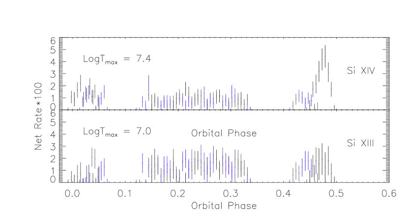
We show the observed and synthetic counts spectra in Figures 4a-4d, the DEM in Figure 5, and list the abundances in Table 3. The line measurements and predicted fluxes are listed in Table 2.
Our method imposes some implicit regularization by smoothing the DEM over a few temperature grid points. In fitting all elements simultaneously, we can couple the DEM over broader temperature ranges and simultaneously derive self consistent relative abundances and DEM. This is necessary to fit the low temperature regions which are not covered by the temperature ranges of the emissivities of the iron ions available with HETGS. By including fluxes from EUV lines (e.g., Fe ix– xvi), we are able to constrain the low temperature portion of the DEM (), which N vii and O vii sample in the HETGS spectrum. We tested consistency by fitting elements independently or in small groups. While fits were of lower quality and limited in temperature range, they were consistent, so we performed the final fit over all elements, ignoring the density-sensitive He-like forbidden and intersystem lines, some strong blends (e.g., Ne ixFe xix 13.4 Å), and some obviously discrepant features which are likely to be either mis-identifications, compromised by blends, or lines for which emissivities are not accurately known.
Since there are poorly quantified systematic uncertainties in the atomic data (and thus emissivities), we repeated the DEM fits with a lower limit to the flux uncertainty of 25% (regardless of the counts) to globally approximate the atomic data systematic errors. The resulting DEM structure was the same, but with appropriately larger uncertainties. This lends confidence that the DEM structure is real and not due to deficiencies in atomic data.
At no point do we formally minimize a binned spectrum against a binned synthetic spectrum. This had been the only option and the norm for low-resolution X-ray spectral modeling with previous missions such as ASCA and ROSAT. There are many ways for such “global” fitting to fail for high-resolution spectra: inaccurate model wavelengths can lead to a mis-match between predicted and observed lines; any spectral region may have features missing from the emissivity database; emissivities may be inaccurate; or continuum bins can dominate , to list a few pitfalls. For these reasons, we prefer a strictly line-based analysis because we can more finely manipulate the features to be fit according to their ionic sequences, density sensitivity, blending, temperature of formation, or any other parameter available in the atomic database. These techniques have long been in use for UV and EUV emission line spectroscopy of coronal plasmas.
The DEM we obtain is dominated by two large peaks, at and . There is a hot tail imposed by the presence of Fe xxv, Fe xxvi, Ca xx, and Ar xviii (within large uncertainty, since the lines are of low signal to noise ratio) and the short wavelength continuum. At , there is a weak peak required by the EUV lines from lower ionization states of iron (ix-xvi) which provide a much better constraint than does the relatively low signal-to-noise detection of N vii (24.8 Å). The overlapping temperature distributions of N and the EUV Fe lines serve to better constrain the abundance of N. We note that the derived DEM is similar to that obtained for the RS CVn system HR 1099 by Drake et al. (2001) based on Chandra HETG spectra, while the double-peaked structure at high temperatures is also reminiscent of the emission measure distributions for AR Lac, HR 1099, II Peg, and other stars derived from EUVE spectra by Griffiths & Jordan (1998) and Sanz-Forcada, Brickhouse & Dupree (2002); the cool bump is also seen in some of the emission measures derived by the latter authors. It is tempting to conclude that the detailed structure in the DEM derived in this study and others does indeed reflect the true source temperature structure. We caution, however, that such apparent structure can also arise as a result of errors in the underlying atomic data (see, e.g., Kashyap & Drake, 1998). In particular, errors in ionization equilibria could plausibly induce spurious structure since such errors would be highly correlated with temperature. We therefore emphasize that detailed interpretation of the DEM structure should proceed with caution.
The very hot portion of the DEM appears to be predominantly due to the flares, since the modulations from Fe xxv and the nearby continuum are nearly 90%. Much of the large peak (–) is contributed by flares, having a modulation greater than 50%. Below 7.0 there is little modulation. This greater variability in the hottest plasma component has been seen in other active stellar coronae (Bowyer, Drake & Vennes, 2000), such as II Peg (Huenemoerder, Canizares & Schulz, 2001) during flaring, in Capella (Brickhouse et al., 2000) in widely separated observations, and in the RS CVn stars studied with EUVE by Sanz-Forcada, Brickhouse & Dupree (2002).
4.3 Abundances
Relative abundances are determined by the DEM fitting procedure, and are strongly correlated with the DEM solution. An element which is isolated in temperature from other ions will be degenerate in the DEM normalization and abundance, since the flux is determined by their product. By fitting all ions simultaneously we remove some of the degeneracy since a series of intermediary strongly overlapping emissivities can couple ions which only overlap slightly. By performing a Monte Carlo iteration we derive an estimate of the range of solutions allowed by measurement uncertainties.
The abundances we derived are listed in Table 3, and we plot them against the first ionization potential (FIP) in Figure 6. The abundances range from about half to about double the Solar photospheric values, with no simple trend with FIP. Neon is about 1.7 times the accepted Solar value and three times the iron abundance. This neon to iron ratio is a fairly reliable determination since the lines form in overlapping temperature ranges and so are relatively independent of the DEM (assuming they form from ions within the same volume). If we average Al and Ca at the lowest FIP, we find them near Solar, and significantly different from the average of Fe, Mg, and Si. Al and Ca form in the same temperature range as Si, so this difference is also relatively independent of the details of the DEM.
The photospheric abundances of AR Lac (Gehren, Ottmann & Reetz, 1999) of iron, silicon, and magnesium (all low FIP elements) are systematically higher than the coronal values. Taking the error-weighted means, we find the relative abundance to be in the coronae, as compared to in the photosphere. The average of the lowest FIP elements, Al and Ca, is , which is comparable to the photospheric value.
Kaastra et al. (1996) and Singh, White & Drake (1996) analyzed the same ROSAT and ASCA data with different methods, but obtained statistically identical results for everything but neon. Their values were about half of ours: (again averaging over Fe, Si, Ca, and Mg). The latter authors gave a good synopsis of the systematic uncertainties in low resolution spectral fits and do show how changes of 50% can arise from fitting different spectral regions. Both studies also obtained values systematically lower than ours for all other elements fit (S, O, N, Ar, Ne). Global fits to low-resolution Beppo-SAX spectra of AR Lac by Rodonò et al. (1999) obtained an average metal abundance of 0.66, similar to our values for Fe, Si, S, Mg, and O.
In comparison to previous measurements from low resolution data, we are most discrepant with Singh, White & Drake (1996) in the sulfur abundance, which they claimed was robust even for low resolution data, and also differ greatly in Al and Ca. We provide a more robust nitrogen abundance, for which they suspected large calibration systematics. The high FIP element abundances are near (N, Ar) to above (Ne) Solar photospheric values; while there are no photospheric measurements for these elements for AR Lac, it seems likely that they follow the approximately solar values for the elements studied by Gehren, Ottmann & Reetz (1999).
4.4 Line Shapes
Both stellar components of AR Lac have been seen to be X-ray active (Walter, Gibson & Basri, 1983; Siarkowski et al., 1996). We have not been able to detect eclipses with our limited phase coverage, but the spectral resolution and phase coverage do permit us to search for line profile variations. At quadrature, the radial velocity separation of the binary components is (see Gehren, Ottmann & Reetz, 1999, for a collation of system parameters). The instrumental full-width, half-maximum (FWHM) of 0.02 Å for MEG and 0.01 Å for HEG yields at O viii (19 Å) and for HEG at Fe xvii (15 Å). We fit the summed quadrature spectra (OID 6 and 9) with one or two instrumental profiles (no thermal or turbulent components included), and with a single broadened Gaussian convolved with the instrumental response. The lines were not well fit by single instrumental profiles. Equally good fits could be obtained with either a single Gaussian with a dispersion of about 0.005–0.01 Å, or by two Gaussians. The O viii two-Gaussian fit is close to the separation expected if both stars are active and the activity is localized near their respective photospheres: the 90% velocity limits are at about the instrumental resolution and overlap the orbital velocities, for the G star, and for the K star (numbers in parenthesis are 90% confidence limits). These values are in reasonable agreement with the orbital velocities of and , respectively, with a range within the observation.
To test for broadening in a way which does not depend on the calibration of the instrumental profile, we compared line profiles between the quadrature and conjunction phases. Both the MEG O viii and HEG Ne-Fe 12Å blend were broader than the instrumental profile at quadrature, and were consistent with the instrumental profile at eclipses. We show the profiles and differences in Figure 7.
4.5 Density
The helium-like triplet lines are well known density diagnostics (Gabriel & Jordan, 1969, 1973; Pradhan & Shull, 1981; Porquet & Dubau, 2000). The critical densities increase with atomic number and are sensitive over the ranges in of about 10–12 for O vii (, 21.8, 22.1, ), 11–13 for Ne ix (, 13.55, 13.70, ), and 12–14 for Mg xi (, 9.23, 9.31, ), which span ranges of interest for coronal plasmas (wavelengths refer to the resonance, intersystem, and forbidden lines, respectively). The density determination depends upon flux ratios including the weak intersystem lines. Positive detection requires high signal, accurate continuum, and resolution of blends. If we examine the spectra (Figure 4a), we see that the continuum is fairly well modeled, so this is not the limiting factor in our measurements. The model significantly underestimates the Ne ix (Figure 4b) and marginally overestimates O vii (Figure 4d) forbidden lines. The Mg xi resonance and forbidden lines match well (Figure 4b).
None of our ratios give a good density constraint: O vii is weak, Ne ix is seriously blended with Fe and is listed here only for completeness, and the Mg xi intersystem line is weak and possibly blended with high- Ne x H-like transitions. The formal ratios indicate logarithmic densities () of about 10.8 from oxygen, but with 90% uncertainties which span the range from 9–12; for neon, 11 with 90% uncertainties up to 11.5; for magnesium, 12.2 with a 90% upper limit of about 12.8. Neon and magnesium can be considered to define upper limits, but the lower limits are unconstrained. The neon intersystem line could be up to about 30% iron blends (Ness, 2002, Ness et al., 2003, in preparation), which would lower the upper limit somewhat.
Hence, we tentatively conclude that we have detected densities on the order of , high enough to affect O vii and Ne ix ratios, but not Mg xi. There is no reason, however, for the values to be identical for different ions, since they form at different temperatures. Without better measurements of the intersystem lines, we do not have data to constrain more rigorously.
5 Discussion
The high resolution X-ray spectrum of AR Lac provides a wealth of new information about the system. While we have derived more detailed emission measure models and abundances than possible from low resolution data, there are still inadequacies in the models and significant problems to be solved. We must remember that there are two stars’ coronae involved, and that they are highly variable, making comparison with other epochs difficult. The composite nature is not a problem for derivation of emission measures since that quantity does not assume any geometric structure. Interpretation of the emission measure, however, does require information or assumptions about the geometrical distribution of plasma.
The line widths, being barely resolved by HETGS, show that both stars are active, as has long been known from the first X-ray observations (Walter, Gibson & Basri, 1983) as well as from spectroscopy in the ultraviolet (Neff et al., 1989; Pagano et al., 2001) and optical (Frasca et al., 2000). Spatial structure can be derived from line velocities or occultations. The only conclusive modulation is from flares, which have high enough frequency and duration (also noted by Pagano et al., 2001, for Mg ii) to make it very difficult to infer spatial structure. Prior studies suggested the G-star to have a compact and uniform chromosphere, and compact but highly structured corona (Pagano et al., 2001, eg). The current lack of modulation during primary eclipse egress coupled with line broadening at quadrature is consistent with this view. The modulation seen by Siarkowski et al. (1996) seems to be ruled out; their ASCA light curves showed a deep and long primary minimum, which they modeled as extended emitting structures between the two stars. Whether such extended material is indeed present will require better phase coverage at different epochs as well as comparison to coronal models in stars which should not have binary interaction. The high frequency and amplitude of flare variability, however, may mean that image reconstruction of the corona is not feasible (Pease et al., 2002, Drake et al., 2003 (in preparation)).
The DEM and abundance model does predict the spectrum reasonably well (see Figure 4a), but there are still some very large discrepancies for individual lines. Some iron line intensities are well modeled, but others exhibit significant discrepancies. For example: Fe xviii is significantly stronger in the model, while the neighboring blend of Fe xviii , Fe xx is well modeled in the predicted two-to-one ratio. The Fe xvii lines, as a series, are also poorly fit: pair model is slightly weak, model is slightly strong, while the model is nearly twice as strong as the data. This latter discrepancy was also noted for II Peg (Huenemoerder, Canizares & Schulz, 2001). Instead of interpreting the apparent weakness of the line as opacity, we suspect that the emissivities may need revision. The new Fe L-shell calculations of Gu (2002) and by Doron & Behar (2002) indicate that some ratios may differ from earlier calculations by about a factor of 1.5. We are working to include updated emissivities into the synthetic spectrum.
There could also be deficiencies in the DEM and abundance model. We could increase the model strength of Fe xvii by increasing the DEM on the low-temperature side of its emissivity distribution (–), so as to minimize the affect on Fe xviii. This, however, would have a ripple of side affects: the abundance of Mg and Ne would have to be reduced, but enhancing the cool DEM would also change the ratios of H-like Mg xii and Ne x to their He-like states, since the H-like emissivities span the hot peak of the DEM. The emissivities of neon, in turn, overlap significantly with those of oxygen, and so forth. We have already implicitly optimized the balance of abundances in the minimization. However, there may be local minima, or our solution may be skewed by erroneous iron emissivities, or may be too smooth to find very sharp temperature structure. Line blending is also a significant problem, and will require a non-local approach in which isolated lines of a blending species are used to predict the contribution of that species to blended features. We have also assumed that each stellar binary component has the same composition, which might be reasonable but is unverified. Future efforts will address these issues.
The normalized line flux residuals () are plotted in Figure 8. The scatter is quite large, with . The Fe xvii lines form near –, and we can see that we have lines both stronger and weaker than the model, as well as a number which are well fit. In addition to the significance of deviations, the bottom panel of the figure shows the flux ratio to the model, which indicates the percentage deviations. We note that the reduced of the spectral energy distribution itself is about 1.0; this is misleading, because it is dominated by a large number of well modeled continuum bins with relatively low signal-to-noise ratios. This illustrates the problem that minimization of a model against a binned spectrum instead of against just the extracted line fluxes places less statistical weight on spectral lines thought to be useful diagnostics, and so devalues the line flux information.
There is at least one other potential source of error in the DEM modeling. We have assumed collisional ionization equilibrium (CIE), in which collisional excitation and ionization from the ground state, followed by radiative decay, recombination, and di-electronic recombination are the dominant processes. We have previously argued (Huenemoerder, Canizares & Schulz, 2001) that this is acceptable even if there is a large flare contribution to the flux, since most lines are expected to thermalize quickly (Golub, Hartquist & Quillen, 1989; Mewe et al., 1985; Doschek et al., 1980). That CIE is valid in all regions of the plasma, though, is an assumption. If flaring is very frequent, or if the apparently quiescent emission were to arise as a result of a superposition of many unresolved, weaker flares, then the plasma might be driven out of CIE. In this regard, improving the model is not a trivial proposition, requiring a detailed attention to each ion series in conjunction with quality assessment of model emissivities and more rigorous incorporation of atomic data uncertainties (including uncertainties in the ion populations) to determine whether or not the data are indeed well-described by the standard optically-thin plasma in thermal equilibrium. We will accept the current DEM and model parameters as the best available, given these caveats.
The abundance trends found in other systems show that low FIP species are sub-Solar, while high FIP elements (neon) which have enhanced abundance (Huenemoerder, Canizares & Schulz, 2001; Drake et al., 2001; Audard, Güdel & Mewe, 2001; Brinkman et al., 2001; Güdel et al., 2001a, b). However, we find that the lowest FIP elements have intermediate abundances, as does the high FIP element Ar, relative to the other elements. AR Lac seems to be more moderate in terms of abundance anomalies compared to other active stars like II Peg or HR 1099, being less deficient in iron, and having a lower neon abundance ratio to iron (see Kastner et al., 2002; Huenemoerder, 2002, for collections of HETGS spectra qualitatively ordered by iron to neon abundance ratio).
The trend of increasing abundance with FIP is opposite what has been seen in the Solar corona (see, e.g., Feldman & Laming, 2000; Feldman, 1992; Feldman, Widing & Lund, 1990, for reviews). FIP-based fractionation is believed to occur in the stellar chromosphere where low FIP species are predominantly ionized while high FIP species remain neutral. However, there is as yet no widely accepted quantitative explanation of the solar FIP effect. The new generation of stellar observations from Chandra and XMM-Newton have provided new challenges for future models. The abundances derived here for AR Lac further complicate the picture with enhanced abundances for elements with both low and high FIP, relative to intermediate FIP elements.
The integrated emission measure we obtain for the range, –, of , is similar to previous determinations. About one third of the emission measure is in the peak at , about half in the peak at 7.4, 15% in the hot tail, and about 2% in the cool bump at 6.2 (note that Figure 5 plots the DEM integrated over intervals of ). Griffiths & Jordan (1998) derived emission measures from UV, EUV, and X-ray data, and Rodonò et al. (1999), who analyzed SAX data, found temperature components similar to our peak DEM temperatures, and integrated emission measures of about half our value. Singh, White & Drake (1996) also derived similar temperature components and emission measures from ROSAT and ASCA spectra, with an integrated emission value more similar to ours. These diverse observations and analyses over several epochs are remarkably similar, and indicate that the mean activity level of the AR Lac coronae is relatively stable.
If we interpret the emission with a very simple geometric model of a semi-toroidal loop of constant cross section, we can derive a loop height as
| (4) |
in which is the number of identical loops divided by 100, is the ratio of loop radius to length divided by 0.1, is the volume emission measure, is the electron density, and is the stellar radius (see Huenemoerder, Canizares & Schulz, 2001, for a derivation). If we attribute half the emission to each star and use a density of , then the loop heights are 0.08 and 0.04 (in stellar radii, relative to the G- and K-star components, respectively). In other words, the loops are compact; even if there are only 10 loops instead of 100, they only double in height, but if density were also ten times lower, then the extent becomes significant. If we attribute the hot part of the DEM to a single flare loop (since “hot” flux is highly modulated), then that loop height is about 0.2–0.9 times the radius of the G-star, for density values of –; this is significant compared to the size of the binary system (2–15% of the semi-major axis). The simple assumptions of semi-toroidal loop intersecting a planar atmosphere are not valid if loops are large relative to the stellar radius, but this heuristic argument supports the existence of extended coronal structures as has been suggested by several authors (Walter, Gibson & Basri, 1983; Siarkowski et al., 1996; Frasca et al., 2000; Pagano et al., 2001; Trigilio et al., 2001). From radio interferometry, Trigilio et al. (2001) derived a scale for the “core” component of the radio corona of about 0.4 G-star radii, similar to our low-density, few-loop case. Their “halo” component was somewhat more extended, to several stellar radii. It is, however, difficult to make a meaningful comparison between the X-ray and radio extents due to the very different model assumptions and the very uncertain X-ray plasma density determination, and because the radio and X-ray emission to not necessarily originate from the same plasma.
In contrast to the spectral behavior, the light curves at various epochs can be quite different. The SAX light curve (Rodonò et al., 1999) showed much structure, with a rotational modulation, a short eclipse, and frequent and short flares. In contrast, the ASCA light curve (Siarkowski et al., 1996) was relatively smooth and showed broad and deep primary eclipse and broad, shallow secondary eclipse. Rodonò et al. (1999) summarize and compare many of the X-ray observations. Some aspects of the data are quite confusing and challenging to explain. For example, the SAX data show a narrow dip during primary eclipse, beginning after second contact (G-star photosphere fully eclipsed), and returning to the higher level before third contact (G-star photosphere fully egressed). This is not consistent with their interpretation that the G-star corona is compact, since the feature would have to be trailing the G-star to make ingress constant in flux, yet leading on egress. Instead, there must be other emerging or erupting structures which could be on either star. Our highly non-repeatable light curves show the extreme difficulty of interpreting variability as rotational modulation or eclipses of stable structures, as was also noted by Pease et al. (2002) for EUV variability.
The flux of AR Lac integrated from – Å is . For a distance of 42 pc, the band luminosity is . This also represents the time-averaged value over the observation, which is strongly biased to the longer quadrature integrations at lower count rate. For short times, the luminosity can be several times higher; the flare of OID 7 emitted about . This is a typical size for RS CVn binaries (e.g. Maggio et al., 2000; Huenemoerder, Canizares & Schulz, 2001) but there have been flares two orders of magnitude larger (Ottmann & Schmitt, 1994; Kuerster & Schmitt, 1996). Perhaps the flare we missed in X-rays was of such a magnitude, given the large X-ray to EUV enhancement ratio we see near orbit 2.4 (see Figure 2, top panel).
Detailed independent modeling of flare and non-flare states, while scientifically interesting in terms of temperature and abundance structure, unfortunately requires better statistics than we have in these data. The larger X-ray flare of OID 7, while significant in the light curve, is relatively short for DEM analysis — much of the count-rate change is from the continuum. The EUVE data, even binned over the entire observation, serve primarily to constrain the low temperature emission since the signal is so much weaker than the HETGS data where lines overlap in formation temperature. We also looked for spectral differences near phase 0.15 between OID 6 and 9, but signal was not adequate, even for summed line fluxes. The line modulation shown in Figure 3 is our low-signal proxy for the detailed model. Time-dependent DEM and abundance modeling of flares will have to await larger events.
We might expect large flares to result in line shifts or excess broadening due to velocity fields. In Figure 7 we show quadrature and conjunction profiles for two lines, O viii and Ne x, which are near the highest resolutions obtained with HETGS. These features, however, form at relatively low temperatures and are relatively un-modulated by the flares (see Figure 3). We have attributed the broadening in O viii to orbital effects. Ne x is interesting because the conjunction profile shows a marginal blueshift, and these phases were most affected by flares. Ayres et al. (2001) tentatively detected a transient blueshift in Ne x in HR 1099, coincident with a UV flare; there was no corresponding X-ray flare detected. We likewise find the effect inconclusive due to conflicting information and marginal data quality. However, the tentative result is intriguing and should foster further observations and more sophisticated analyses.
6 Conclusions
We have presented an analysis of high resolution X-ray and EUV spectra and photometry of the bright eclipsing RS CVn system AR Lac. While our results are qualitatively similar to those of earlier studies, the high resolution X-ray line spectra have allowed us to obtain a significantly more detailed glimpse of the coronal temperature structure and abundances.
The X-ray and EUV spectra show that the coronae of this system are characterized by complicated structure and variability. The overall activity level is similar to that determined from previous observations. The hot portion of the DEM is strongly modulated by flares, whereas the cooler portion appears relatively quiescent. The flare modulation is either frequent and large enough to hide eclipses, or the dominant coronal structures are of polar origin and are not rotationally modulated. The steadily emitting structures could be compact if the density estimate of is accurate, whereas if the emission from the X-ray flare is from a single loop at this density, then it would be significantly extended. This ambiguity in interpretation illustrates the importance of reliable plasma density estimates and underscores the difficulty in obtaining such estimates, even from high-quality Chandra HETG observations. Given the high resolution of the HETGS, we have determined that both stellar components of the system contribute significantly to the X-ray emission. The quadrature line profiles are consistent with the K- and G-stars being equally bright.
Coronal abundances show some similarities with those found for other RS CVn stars but differ substantially in detail: the highest and lowest FIP species both appear to have higher abundances relative to intermediate FIP ions. For AR Lac, the intermediate FIP abundances are below measured photospheric values.
References
- Anders & Grevesse (1989) Anders, E., & Grevesse, N., 1989, Geochim. Cosmochim. Acta, 53, 197
- Audard, Güdel & Mewe (2001) Audard, M., Güdel, M., & Mewe, R., 2001, A&A, 365, L318
- Ayres et al. (2001) Ayres, T. R., Brown, A., Osten, R. A., Huenemoerder, D. P., Drake, J. J., Brickhouse, N. S., & Linsky, J. L., 2001, ApJ, 549, 554
- Bowyer, Drake & Vennes (2000) Bowyer, S., Drake, J. J., & Vennes, S., 2000, ARA&A, 38, 231
- Brickhouse et al. (2000) Brickhouse, N. S., Dupree, A. K., Edgar, R. J., Liedahl, D. A., Drake, S. A., White, N. E., & Singh, K. P., 2000, ApJ, 530, 387
- Brickhouse et al. (1999) Brickhouse, N. S., Dupree, A. K., Sanz-Forcada, J., Drake, S. A., White, N. E., & Singh, K. P., 1999, Bulletin of the American Astronomical Society, 31, 706
- Brinkman et al. (2001) Brinkman, A. C., et al., 2001, A&A, 365, L324
- Christian et al. (1996) Christian, D. J., Drake, J. J., Patterer, R. J., Vedder, P. W., & Bowyer, S., 1996, AJ, 112, 751
- Craig & Brown (1976) Craig, I. J. D., & Brown, J. C., 1976, A&A, 49, 239
- Doron & Behar (2002) Doron, R., & Behar, E., 2002, ApJ, 574, 518
- Doschek et al. (1980) Doschek, G. A., Feldman, U., Kreplin, R. W., & Cohen, L., 1980, ApJ, 239, 725
- Drake et al. (2001) Drake, J. J., Brickhouse, N. S., Kashyap, V., Laming, J. M., Huenemoerder, D. P., Smith, R., & Wargelin, B. J., 2001, ApJ, 548, L81
- Feldman (1992) Feldman, U., 1992, Phys. Scr, 46, 202
- Feldman & Laming (2000) Feldman, U., & Laming, J., 2000, Phys. Scr, 61, 222
- Feldman, Widing & Lund (1990) Feldman, U., Widing, K. G., & Lund, P. A., 1990, ApJ, 364, L21
- Frasca et al. (2000) Frasca, A., Marino, G., Catalano, S., & Marilli, E., 2000, A&A, 358, 1007
- Güdel et al. (2001a) Güdel, M., et al., 2001a, A&A, 365, L336
- Güdel et al. (2001b) Güdel, M., Audard, M., Magee, H., Franciosini, E., Grosso, N., Cordova, F. A., Pallavicini, R., & Mewe, R., 2001b, A&A, 365, L344
- Gabriel & Jordan (1969) Gabriel, A. H., & Jordan, C., 1969, MNRAS, 145, 241
- Gabriel & Jordan (1973) Gabriel, A. H., & Jordan, C., 1973, ApJ, 186, 327
- Gehren, Ottmann & Reetz (1999) Gehren, T., Ottmann, R., & Reetz, J., 1999, A&A, 344, 221
- Golub, Hartquist & Quillen (1989) Golub, L., Hartquist, T. W., & Quillen, A. C., 1989, Sol. Phys., 122, 245
- Griffiths & Jordan (1998) Griffiths, N. W., & Jordan, C., 1998, ApJ, 497, 883
- Gu (2002) Gu, M. F., 2002, ApJ, 579, L103
- Haisch, Bowyer & Malina (1993) Haisch, B., Bowyer, S., & Malina, R. F., 1993, Journal of the British Interplanetary Society, 46, 331
- Houck & Denicola (2000) Houck, J. C., & Denicola, L. A., 2000, in ASP Conf. Ser. 216: Astronomical Data Analysis Software and Systems IX, Vol. 9, 591
- Hubeny & Judge (1995) Hubeny, V., & Judge, P. G., 1995, ApJ, 448, L61
- Huenemoerder (2002) Huenemoerder, D. P., 2002, in High Resolution X-ray Spectroscopy with XMM-Newton and Chandra (http://www.mssl.ucl.ac.uk/gbr/rgs_workshop)
- Huenemoerder, Canizares & Schulz (2001) Huenemoerder, D. P., Canizares, C. R., & Schulz, N. S., 2001, ApJ, 559, 1135
- Judge, Hubeny & Brown (1997) Judge, P. G., Hubeny, V., & Brown, J. C., 1997, ApJ, 475, 275
- Kaastra et al. (1996) Kaastra, J. S., Mewe, R., Liedahl, D. A., Singh, K. P., White, N. E., & Drake, S. A., 1996, A&A, 314, 547
- Kashyap & Drake (1998) Kashyap, V., & Drake, J. J., 1998, ApJ, 503, 450
- Kastner et al. (2002) Kastner, J. H., Huenemoerder, D. P., Schulz, N. S., Canizares, C. R., & Weintraub, D. A., 2002, ApJ, 567, 434
- Kimble et al. (1993) Kimble, R. A., Davidsen, A. F., Long, K. S., & Feldman, P. D., 1993, ApJ, 408, L41
- Kuerster & Schmitt (1996) Kuerster, M., & Schmitt, J. H. M. M., 1996, A&A, 311, 211
- Maggio et al. (2000) Maggio, A., Pallavicini, R., Reale, F., & Tagliaferri, G., 2000, A&A, 356, 627
- Marino et al. (1998) Marino, G., Catalano, S., Frasca, A., & Marilli, E., 1998, Informational Bulletin on Variable Stars, 4599, 1
- Mazzotta et al. (1998) Mazzotta, P., Mazzitelli, G., Colafrancesco, S., & Vittorio, N., 1998, A&AS, 133, 403
- McIntosh, Brown & Judge (1998) McIntosh, S. W., Brown, J. C., & Judge, P. G., 1998, A&A, 333, 333
- Mewe et al. (1985) Mewe, R., Lemen, J. R., Peres, G., Schrijver, J., & Serio, S., 1985, A&A, 152, 229
- Montes et al. (1997) Montes, D., Fernandez-Figueroa, M. J., de Castro, E., & Sanz-Forcada, J., 1997, A&AS, 125, 263
- Neff et al. (1989) Neff, J. E., Walter, F. M., Rodono, M., & Linsky, J. L., 1989, A&A, 215, 79
- Ness (2002) Ness, J., 2002, in High Resolution X-ray Spectroscopy with XMM-Newton and Chandra (http://www.mssl.ucl.ac.uk/gbr/rgs_workshop)
- Ottmann & Schmitt (1994) Ottmann, R., & Schmitt, J. H. M. M., 1994, A&A, 283, 871
- Ottmann, Schmitt & Kuerster (1993) Ottmann, R., Schmitt, J. H. M. M., & Kuerster, M., 1993, ApJ, 413, 710
- Pagano et al. (2001) Pagano, I., Rodonò, M., Linsky, J. L., Neff, J. E., Walter, F. M., Kovári, Z., & Matthews, L. D., 2001, A&A, 365, 128
- Pease et al. (2002) Pease, D., et al., 2002, in ASP Conf. Ser. 277: Stellar Coronae in the Chandra and XMM-Newton Era, Vol. 277, 547
- Perryman et al. (1997) Perryman, M. A. C., et al., 1997, A&A, 323, L49
- Porquet & Dubau (2000) Porquet, D., & Dubau, J., 2000, A&AS, 143, 495
- Pradhan & Shull (1981) Pradhan, A. K., & Shull, J. M., 1981, ApJ, 249, 821
- Raymond & Brickhouse (1996) Raymond, J. C., & Brickhouse, N. C., 1996, Ap&SS, 237, 321
- Rodonò et al. (1999) Rodonò, M., Pagano, I., Leto, G., Walter, F., Catalano, S., Cutispoto, G., & Umana, G., 1999, A&A, 346, 811
- Sanz-Forcada, Brickhouse & Dupree (2002) Sanz-Forcada, J., Brickhouse, N. S., & Dupree, A. K., 2002, ApJ, 570, 799
- Sanz-Forcada, Brickhouse & Dupree (2003) Sanz-Forcada, J., Brickhouse, N. S., & Dupree, A. K., 2003, ApJS, 145, in press
- Siarkowski et al. (1996) Siarkowski, M., Pres, P., Drake, S. A., White, N. E., & Singh, K. P., 1996, ApJ, 473, 470
- Singh, White & Drake (1996) Singh, K. P., White, N. E., & Drake, S. A., 1996, ApJ, 456, 766
- Smith et al. (2001) Smith, R. K., Brickhouse, N. S., Liedahl, D. A., & Raymond, J. C., 2001, ApJ, 556, L91
- Trigilio et al. (2001) Trigilio, C., Buemi, C. S., Umana, G., Rodonò, M., Leto, P., Beasley, A. J., & Pagano, I., 2001, A&A, 373, 181
- Walter et al. (1980) Walter, F. M., Cash, W., Charles, P. A., & Bowyer, C. S., 1980, ApJ, 236, 212
- Walter, Gibson & Basri (1983) Walter, F. M., Gibson, D. M., & Basri, G. S., 1983, ApJ, 267, 665
- Weisskopf et al. (2002) Weisskopf, M. C., Brinkman, B., Canizares, C., Garmire, G., Murray, S., & Van Speybroeck, L. P., 2002, PASP, 114, 1
- White et al. (1994) White, N. E., et al., 1994, PASJ, 46, L97
- White et al. (1990) White, N. E., Shafer, R. A., Parmar, A. N., Horne, K., & Culhane, J. L., 1990, ApJ, 350, 776
| OID | Start Date & Time | ExposureaaExposure time is in ks. | PhasebbPhase is computed for the exposure start and stop times using the ephemeris of Perryman et al. (1997). At phase 0.0, the G-star is totally eclipsed. |
|---|---|---|---|
| 6 | 2000-09-11T22:05:13 | 32.7 | 0.14–0.34 |
| 7 | 2000-09-16T11:48:03 | 7.7 | 0.48–0.52 |
| 8 | 2000-09-15T14:18:04 | 9.5 | 0.98–0.02 |
| 9 | 2000-09-17T20:02:12 | 32.5 | 0.15–0.35 |
| 10 | 2000-09-20T09:28:11 | 7.5 | 0.42–0.46 |
| 11 | 2000-09-19T14:31:14 | 7.5 | 0.02–0.06 |
| MnemonicaaThe mnemonic is a convenience for uniquely naming each feature. It is comprised of the element and ion (in Arabic numerals) followed by a string indicating a wavelength and the wavelength (e.g., w16.78), or a code for the hydrogen-like (“H”) and helium-like “He” series, “L” for Lyman transition, one of “a”, “b”, “g”, “d”, or “e” for series lines , and “r”, “i”, or “f” for resonance, intersystem, or forbidden lines. | Ion | bbAverage logarithmic temperature [Kelvins] of formation, defined as the first moment of the emissivity distribution. | ccTheoretical wavelengths of identification (from APED), in Å. If the line is a multiplet, we give the wavelength of the strongest component. | ddMeasured wavelength, in Å (uncertainty is in mÅ). | eeEmitted source line flux is times the tabulated value in . | ffModel line flux is times the tabulated value in . | ggLine flux residual, . | hh. |
|---|---|---|---|---|---|---|---|---|
| Fe26HLa | Fe XXVI | 8.1 | 1.781 | 1.782 (156.2) | 3.48 (4.43) | 4.40 | -0.92 | -0.2 |
| Fe25HeLa | Fe XXV | 7.8 | 1.861 | 1.859 ( 1.9) | 23.70 (7.14) | 25.95 | -2.25 | -0.3 |
| Ca20HLa | Ca XX | 7.8 | 3.021 | 3.020 (110.5) | 1.97 (1.19) | 1.90 | 0.06 | 0.1 |
| Ca19HeLaB | Ca XIX | 7.5 | 3.198 | 3.192 ( 18.1) | 8.10 (2.74) | 8.37 | -0.27 | -0.1 |
| Ar17HeLb | Ar XVII | 7.4 | 3.365 | 3.365 ( 4.3) | 3.63 (1.89) | 1.16 | 2.47 | 1.3 |
| Ar18HLa | Ar XVIII | 7.7 | 3.734 | 3.732 ( 4.9) | 4.44 (2.08) | 5.57 | -1.13 | -0.5 |
| Ar17HeLar | Ar XVII | 7.4 | 3.949 | 3.950 ( 2.4) | 9.32 (2.49) | 8.91 | 0.41 | 0.2 |
| Ar17HeLai | Ar XVII | 7.3 | 3.968 | 3.969 ( 5.6) | 5.49 (2.36) | 2.32 | 3.17 | 1.3 |
| S16HLb,Ar17HeLafiiS xvi 3.991 Å is blended with Ar xvii 3.994 Å in about equal strengths for the model DEM. | Ar XVII | 7.5 | 3.992 | 3.994 ( 3.5) | 6.10 (2.19) | 6.12 | -0.02 | -0.0 |
| S16HLa | S XVI | 7.6 | 4.730 | 4.730 ( 0.9) | 23.60 (3.42) | 26.05 | -2.45 | -0.7 |
| S15HeLar | S XV | 7.2 | 5.039 | 5.039 ( 1.0) | 24.85 (3.56) | 26.65 | -1.80 | -0.5 |
| S15HeLai | S XV | 7.2 | 5.065 | 5.065 ( 13.8) | 6.45 (2.80) | 5.83 | 0.61 | 0.2 |
| S15HeLaf | S XV | 7.2 | 5.102 | 5.100 ( 2.4) | 13.59 (3.13) | 8.78 | 4.81 | 1.5 |
| Si14HLb | Si XIV | 7.4 | 5.217 | 5.219 ( 2.2) | 12.83 (3.30) | 8.81 | 4.02 | 1.2 |
| Si14HLa | Si XIV | 7.4 | 6.183 | 6.181 ( 0.4) | 68.89 (2.94) | 62.34 | 6.55 | 2.2 |
| Si13HeLar | Si XIII | 7.0 | 6.648 | 6.648 ( 0.5) | 44.03 (2.28) | 51.71 | -7.68 | -3.4 |
| Si13HeLai | Si XIII | 7.0 | 6.687 | 6.686 ( 1.5) | 8.49 (1.53) | 9.54 | -1.05 | -0.7 |
| Si13HeLaf | Si XIII | 7.0 | 6.740 | 6.740 ( 0.3) | 30.20 (1.99) | 20.64 | 9.56 | 4.8 |
| Mg12HLb | Mg XII | 7.2 | 7.106 | 7.105 ( 0.7) | 13.47 (1.47) | 14.14 | -0.67 | -0.5 |
| Fe24w7.17 | Fe XXIV | 7.4 | 7.169 | 7.170 ( 0.7) | 13.84 (1.45) | 4.33 | 9.51 | 6.6 |
| Al13HLajjAl xiii 1.172 is blended with Fe xxiv 7.169. We have adjusted the Al flux to account for a 25% contribution of Fe for the assumed DEM. | Al XIII | 7.3 | 7.172 | 7.170 ( 0.5) | 11.03 (0.94) | 12.00 | -0.97 | -1.0 |
| Al12HeLar | Al XII | 7.0 | 7.757 | 7.758 ( 1.9) | 7.84 ( 1.35) | 5.51 | 2.33 | 1.7 |
| Mg11HeLb | Mg XI | 6.9 | 7.850 | 7.849 ( 2.6) | 6.00 ( 1.36) | 7.66 | -1.67 | -1.2 |
| Al12HeLaf | Al XII | 6.9 | 7.872 | 7.869 ( 4.5) | 4.71 ( 1.35) | 4.53 | 0.18 | 0.1 |
| Fe24w7.99 | Fe XXIV | 7.4 | 7.991 | 7.989 ( 1.6) | 9.48 ( 1.31) | 13.82 | -4.34 | -3.3 |
| Fe24w8.23 | Fe XXIV | 7.4 | 8.233 | 8.283 ( 4.2) | 3.24 ( 1.32) | 4.96 | -1.71 | -1.3 |
| Fe24w8.28 | Fe XXIV | 7.4 | 8.285 | 8.304 ( 2.5) | 6.57 ( 1.74) | 1.85 | 4.72 | 2.7 |
| Fe23w8.30 | Fe XXIII | 7.2 | 8.304 | 8.318 ( 6.5) | 8.12 ( 1.95) | 8.36 | -0.24 | -0.1 |
| Fe24w8.32 | Fe XXIV | 7.4 | 8.316 | 8.237 ( 1.8) | 5.41 ( 1.30) | 10.09 | -4.68 | -3.6 |
| Mg12HLa | Mg XII | 7.2 | 8.422 | 8.420 ( 0.3) | 98.76 ( 3.20) | 102.70 | -3.94 | -1.2 |
| Fe23w8.81 | Fe XXIII | 7.2 | 8.815 | 8.814 ( 1.7) | 8.34 ( 1.47) | 8.38 | -0.04 | -0.0 |
| Fe22w8.97 | Fe XXII | 7.1 | 8.975 | 8.975 ( 1.3) | 9.95 ( 1.64) | 7.57 | 2.38 | 1.4 |
| Mg11HeLar | Mg XI | 6.8 | 9.169 | 9.168 ( 0.5) | 57.25 ( 3.01) | 59.28 | -2.03 | -0.7 |
| Mg11HeLai | Mg XI | 6.8 | 9.230 | 9.231 ( 2.1) | 14.32 ( 2.06) | 8.99 | 5.33 | 2.6 |
| Mg11HeLaf | Mg XI | 6.8 | 9.314 | 9.313 ( 0.7) | 28.47 ( 2.07) | 26.81 | 1.66 | 0.8 |
| Ne10HLg | Ne X | 7.0 | 9.708 | 9.710 ( 1.2) | 45.64 ( 6.46) | 28.24 | 17.40 | 2.7 |
| Ne10HLb | Ne X | 7.0 | 10.239 | 10.238 ( 0.4) | 85.51 ( 3.80) | 89.03 | -3.52 | -0.9 |
| Fe24w10.62 | Fe XXIV | 7.4 | 10.619 | 10.620 ( 0.9) | 61.70 ( 4.27) | 65.97 | -4.27 | -1.0 |
| Fe24w10.66 | Fe XXIV | 7.4 | 10.663 | 10.661 ( 1.9) | 34.56 ( 3.54) | 34.61 | -0.05 | -0.0 |
| Fe17w10.77 | Fe XVII | 6.8 | 10.770 | 10.768 ( 2.5) | 10.41 ( 2.09) | 9.08 | 1.32 | 0.6 |
| Fe19w10.82 | Fe XIX | 6.9 | 10.816 | 10.814 ( 2.5) | 11.44 ( 2.16) | 11.96 | -0.52 | -0.2 |
| Fe23w10.98 | Fe XXIII | 7.2 | 10.981 | 10.983 ( 1.2) | 44.19 ( 7.54) | 44.10 | 0.09 | 0.0 |
| Fe23w11.02 | Fe XXIII | 7.2 | 11.019 | 11.015 ( 3.8) | 24.62 ( 7.90) | 28.89 | -4.27 | -0.5 |
| Fe24w11.03 | Fe XXIV | 7.4 | 11.029 | 11.031 ( 7.8) | 54.16 ( 9.48) | 42.19 | 11.97 | 1.3 |
| Fe24w11.18 | Fe XXIV | 7.4 | 11.176 | 11.173 ( 0.6) | 72.06 ( 4.36) | 76.20 | -4.14 | -1.0 |
| Fe18w11.33 | Fe XVIII | 6.8 | 11.326 | 11.330 ( 0.9) | 18.26 ( 2.64) | 18.61 | -0.35 | -0.1 |
| Fe18w11.53 | Fe XVIII | 6.8 | 11.527 | 11.529 ( 2.2) | 19.78 ( 3.11) | 12.78 | 7.00 | 2.3 |
| Ne9HeLb | Ne IX | 6.6 | 11.544 | 11.549 ( 1.2) | 28.16 ( 3.37) | 20.24 | 7.92 | 2.3 |
| Fe23w11.74 | Fe XXIII | 7.2 | 11.736 | 11.738 ( 1.1) | 91.55 ( 4.78) | 91.19 | 0.36 | 0.1 |
| Fe22w11.77 | Fe XXII | 7.1 | 11.770 | 11.771 ( 1.1) | 74.99 ( 4.45) | 70.06 | 4.93 | 1.1 |
| Fe17w12.12kkNe x 12.132 Å is blended with Fe xvii 12.124 Å; in the HEG spectrum, the lines are barely resolved, and expected to be about 10% as strong. Their sum has . | Fe XVII | 6.7 | 12.124 | 12.130 ( 0.9) | 251.30 ( 33.48) | 50.17 | 201.13 | 6.0 |
| Ne10HLakkNe x 12.132 Å is blended with Fe xvii 12.124 Å; in the HEG spectrum, the lines are barely resolved, and expected to be about 10% as strong. Their sum has . | Ne X | 6.9 | 12.135 | 12.139 ( 3.8) | 383.89 ( 33.00) | 633.70 | -249.81 | -7.6 |
| Fe23w12.16 | Fe XXIII | 7.2 | 12.161 | 12.155 ( 1.9) | 56.61 ( 10.70) | 50.26 | 6.35 | 0.6 |
| Fe17w12.27 | Fe XVII | 6.7 | 12.266 | 12.261 ( 3.4) | 27.94 ( 9.27) | 45.09 | -17.16 | -1.9 |
| Fe21w12.28 | Fe XXI | 7.1 | 12.284 | 12.285 ( 0.6) | 137.49 ( 15.15) | 135.90 | 1.59 | 0.1 |
| Fe20w12.58 | Fe XX | 7.0 | 12.576 | 12.574 ( 0.0) | 21.54 ( 3.34) | 22.67 | -1.13 | -0.3 |
| Fe22w12.75 | Fe XXII | 7.1 | 12.754 | 12.751 ( 1.9) | 23.90 ( 3.63) | 25.34 | -1.44 | -0.4 |
| Ne9HeLar | Ne IX | 6.6 | 13.447 | 13.445 ( 0.6) | 132.67 ( 11.30) | 144.90 | -12.23 | -1.1 |
| Fe19w13.50 | Fe XIX | 6.9 | 13.497 | 13.504 ( 0.9) | 69.49 ( 7.51) | 44.98 | 24.50 | 3.3 |
| Fe19w13.52 | Fe XIX | 6.9 | 13.518 | 13.520 ( 0.6) | 81.26 ( 7.61) | 99.15 | -17.89 | -2.4 |
| Ne9HeLai | Ne IX | 6.6 | 13.552 | 13.554 ( 1.9) | 36.59 ( 4.81) | 19.55 | 17.04 | 3.5 |
| Ne9HeLaf | Ne IX | 6.6 | 13.699 | 13.699 ( 0.6) | 110.30 ( 7.00) | 65.60 | 44.70 | 6.4 |
| Fe18w14.26 | Fe XVIII | 6.8 | 14.256 | 14.205 ( 0.3) | 119.10 ( 8.24) | 40.82 | 78.28 | 9.5 |
| Fe20w14.27 | Fe XX | 7.0 | 14.267 | 14.259 ( 1.6) | 48.42 ( 6.15) | 26.94 | 21.48 | 3.5 |
| Fe18w14.53 | Fe XVIII | 6.8 | 14.534 | 14.540 ( 1.3) | 52.72 ( 5.78) | 41.11 | 11.61 | 2.0 |
| O8HLd | O VIII | 6.7 | 14.821 | 14.820 ( 0.0) | 21.59 ( 4.95) | 17.90 | 3.69 | 0.7 |
| Fe17w15.01 | Fe XVII | 6.7 | 15.014 | 15.012 ( 0.6) | 271.60 ( 12.64) | 441.60 | -170.00 | -13.4 |
| Fe19w15.08 | Fe XIX | 6.9 | 15.079 | 15.079 ( 1.3) | 44.58 ( 6.18) | 33.30 | 11.28 | 1.8 |
| O8HLgllO viii 15.18 Å is blended with Fe xix in about equal strengths. | O VIII | 6.7 | 15.176 | 15.180 ( 2.2) | 82.16 ( 8.92) | 40.88 | 41.28 | 4.6 |
| Fe17w15.26 | Fe XVII | 6.7 | 15.261 | 15.261 ( 1.2) | 116.33 ( 9.19) | 124.40 | -8.07 | -0.9 |
| Fe18w15.62 | Fe XVIII | 6.8 | 15.625 | 15.625 ( 1.9) | 42.85 ( 6.16) | 55.81 | -12.96 | -2.1 |
| Fe18w15.82 | Fe XVIII | 6.8 | 15.824 | 15.826 ( 2.2) | 32.92 ( 5.94) | 33.99 | -1.06 | -0.2 |
| Fe18w15.87 | Fe XVIII | 6.8 | 15.870 | 15.869 ( 1.9) | 33.99 ( 6.10) | 18.03 | 15.96 | 2.6 |
| O8HLbmmO viii 16.01 Å is blended with Fe xviii; Fe xviii 15.62 Å has a similar theoretical emissivity distribution to Fe xviii 16.01, so we have subtracted the latter’s flux from the measured O viii to approximate the net O viii flux. | O VIII | 6.7 | 16.006 | 16.005 ( 0.9) | 130.71 ( 26.12) | 127.10 | 3.61 | 0.1 |
| Fe18w16.07 | Fe XVIII | 6.8 | 16.071 | 16.072 ( 0.9) | 99.86 ( 9.51) | 77.00 | 22.86 | 2.4 |
| Fe19w16.11 | Fe XIX | 6.9 | 16.110 | 16.106 ( 3.4) | 25.85 ( 6.84) | 43.53 | -17.68 | -2.6 |
| Fe18w16.16 | Fe XVIII | 6.8 | 16.159 | 16.168 ( 3.7) | 21.99 ( 6.20) | 31.16 | -9.17 | -1.5 |
| Fe17w16.78 | Fe XVII | 6.7 | 16.780 | 16.773 ( 1.2) | 168.16 ( 12.85) | 193.60 | -25.44 | -2.0 |
| Fe17w17.05 | Fe XVII | 6.7 | 17.051 | 17.049 ( 0.6) | 236.37 ( 14.89) | 232.30 | 4.07 | 0.3 |
| Fe17w17.10 | Fe XVII | 6.7 | 17.096 | 17.094 ( 0.6) | 222.20 ( 14.59) | 210.10 | 12.10 | 0.8 |
| Fe18w17.62 | Fe XVIII | 6.8 | 17.623 | 17.619 ( 2.5) | 37.17 ( 8.06) | 55.56 | -18.39 | -2.3 |
| O7HeLb | O VII | 6.4 | 18.627 | 18.625 ( 7.5) | 25.34 ( 8.67) | 15.36 | 9.98 | 1.2 |
| O8HLa | O VIII | 6.7 | 18.970 | 18.968 ( 2.0) | 810.96 ( 87.37) | 858.80 | -47.84 | -0.5 |
| O7HeLar | O VII | 6.3 | 21.602 | 21.601 ( 1.9) | 125.43 ( 22.71) | 128.90 | -3.47 | -0.2 |
| O7HeLai | O VII | 6.3 | 21.802 | 21.804 (156.2) | 23.69 ( 15.62) | 18.70 | 5.00 | 0.3 |
| O7HeLaf | O VII | 6.3 | 22.098 | 22.095 ( 11.3) | 43.55 ( 19.63) | 76.97 | -33.42 | -1.7 |
| N7HLa | N VII | 6.5 | 24.782 | 24.780 ( 3.1) | 132.88 ( 25.49) | 137.20 | -4.32 | -0.2 |
| Fe18w93.92 | Fe XVIII | 6.8 | 93.923 | 93.920 ( 3.0) | 661.91 ( 118.20) | 711.70 | -49.79 | -0.4 |
| Fe19w101.55 | Fe XIX | 6.9 | 101.550 | 101.510 ( 40.0) | 259.18 ( 78.54) | 235.00 | 24.18 | 0.3 |
| Fe18w103.94 | Fe XVIII | 6.8 | 103.937 | 103.940 ( -3.0) | 250.63 ( 86.43) | 260.50 | -9.87 | -0.1 |
| Fe19w108.37 | Fe XIX | 6.9 | 108.370 | 108.230 (140.0) | 796.49 ( 124.45) | 900.40 | -103.91 | -0.8 |
| Fe19w109.97 | Fe XIX | 6.9 | 109.970 | 109.790 (180.0) | 217.01 ( 74.83) | 120.20 | 96.81 | 1.3 |
| Fe20w110.63 | Fe XX | 7.0 | 110.630 | 110.830 (-200.0) | 181.00 ( 78.69) | 42.81 | 138.19 | 1.8 |
| Fe22w114.41 | Fe XXII | 7.1 | 114.410 | 114.430 (-20.0) | 339.81 ( 94.39) | 358.90 | -19.09 | -0.2 |
| Fe20w118.66 | Fe XX | 7.0 | 118.660 | 118.520 (140.0) | 284.33 ( 98.05) | 528.10 | -243.77 | -2.5 |
| Fe19w120.00 | Fe XIX | 6.9 | 120.000 | 119.810 (190.0) | 177.00 ( 93.16) | 243.60 | -66.60 | -0.7 |
| Fe20w121.83 | Fe XX | 7.0 | 121.830 | 121.750 ( 80.0) | 553.19 ( 134.93) | 1029.00 | -475.81 | -3.5 |
| Fe21w128.73 | Fe XXI | 7.0 | 128.730 | 128.560 (170.0) | 1445.10 ( 190.13) | 1520.00 | -74.90 | -0.4 |
| Fe22w135.78 | Fe XXII | 7.1 | 135.780 | 135.590 (190.0) | 1168.80 ( 201.53) | 799.30 | 369.50 | 1.8 |
| Fe21w142.16 | Fe XXI | 7.0 | 142.215 | 142.380 (-165.0) | 437.97 ( 199.07) | 139.70 | 298.27 | 1.5 |
| Fe9w171.07 | Fe IX | 5.8 | 171.073 | 170.950 (123.0) | 1240.10 ( 539.18) | 1377.00 | -136.90 | -0.3 |
| Fe24w192.04 | Fe XXIV | 7.3 | 192.017 | 192.560 (-543.0) | 7453.50 ( 837.47) | 3120.00 | 4333.50 | 5.2 |
| Fe12w195.12 | Fe XII | 6.1 | 195.118 | 195.920 (-802.0) | 1964.50 ( 577.78) | 1759.00 | 205.50 | 0.4 |
| Fe24w255.10 | Fe XXIV | 7.3 | 255.090 | 254.730 (360.0) | 3737.00 (1038.03) | 1655.00 | 2082.00 | 2.0 |
| Fe15w284.15 | Fe XV | 6.4 | 284.160 | 284.110 ( 50.0) | 1945.40 ( 926.38) | 3024.00 | -1078.60 | -1.2 |
| Fe16w335.41 | Fe XVI | 6.5 | 335.410 | 334.210 (1200.0) | 8023.00 (1573.00) | 3892.00 | 4131.00 | 2.6 |
| Fe16w360.80 | Fe XVI | 6.5 | 360.761 | 358.690 (2071.0) | 3941.00 (1115.90) | 2004.00 | 1937.00 | 1.7 |
Note. — Values given in parentheses are the one standard deviation uncertainties on the preceding quantity. Lines with wavelength greater than 30 Å are EUVE data.
| Element | FIPaaFIP is the first ionization potential in eV. | CoronabbCoronal abundances are fractional relative to the Solar abundances of Anders & Grevesse (1989). Numbers in parentheses are one standard deviation uncertainties determined from Monte Carlo fitting. | PhotosphereccPhotospheric abundances from Gehren, Ottmann & Reetz (1999). |
|---|---|---|---|
| N | 14.53 | 1.2 (0.3) | |
| O | 13.62 | 0.6 (0.1) | |
| Ne | 21.56 | 1.6 (0.3) | |
| Mg | 7.65 | 0.7 (0.1) | 1.0 (0.2) |
| Al | 5.99 | 1.3 (0.3) | |
| Si | 8.15 | 0.6 (0.1) | 1.3 (0.9) |
| S | 10.36 | 0.6 (0.1) | |
| Ar | 15.75 | 1.0 (0.2) | |
| Ca | 6.11 | 1.0 (0.3) | 1.3 (0.4) |
| Fe | 7.87 | 0.5 (0.1) | 1.0 (0.2) |
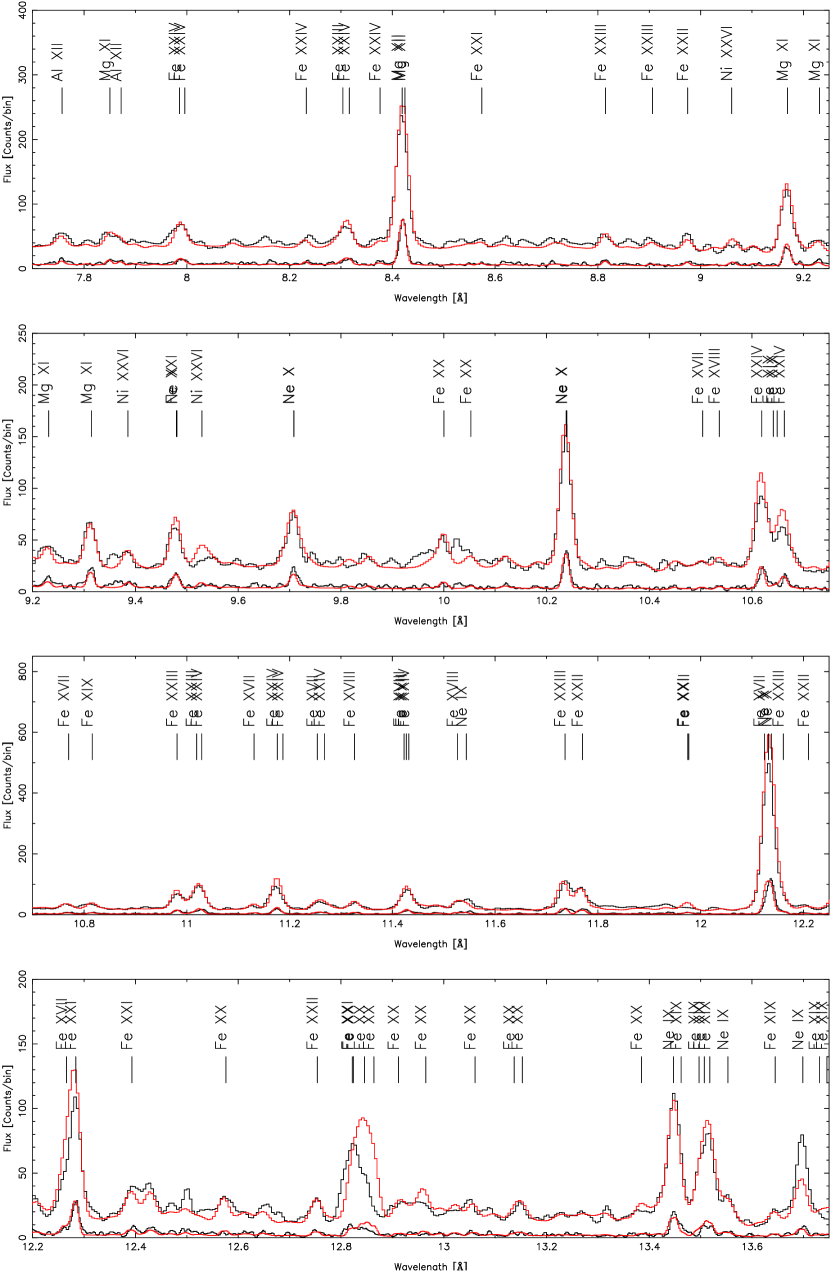
This is the energy flux density spectrum for the summed HEG and MEG first orders for all observations, totalling 97 ks. The spectrum has been smoothed by convolving it with a Gaussian kernel of dispersion 0.005Å. Significant lines have been marked. The strength of the short-wavelength continuum ( Å) and the number of high-excitation iron lines are indicative of the presence of very hot plasma up to about , while presence of N vii, O vii, O viii, and Ne ix indicates cooler plasma, near .
We show the light curve over the six observations in several forms. The top panel shows the count rate against a binary system orbit number, with zero defined as a primary conjunction (HJD 2448501.1232). Given the orbital period of 1.98318 days, an orbit is 171 ks. Both MEG and HEG orders to (excluding the zero order, which is saturated) were summed into 0.5 ks bins over the wavelength range of 1.7–25 Å. Data are labeled by their OID. The EUVE light curve is plotted with small open squares (colored green in the electronic edition), and runs from about orbit 1.6 to 3.0, and is in 0.6 ks bins. The EUVE data’s error bars, which have been omitted for clarity, are all less than 15%. Note the small EUV flux enhancement during the flare in OID 7. The next panel shows the same data, but phase-folded, and only over the phase interval observed by Chandra. The dotted curve (solid orange in the electronic edition) is a simple occultation model for uniform disks of equal surface brightness to show where photospheric eclipses occur, arbitrarily scaled to exaggerate the eclipses. The primary eclipse () is total, and the secondary is annular. The EUVE data are the sparse set of squares running along the bottom (colored green in the electronic edition). The bottom pair of graphs show the light curves for narrow bands around Si xiv (6.16–6.22 Å), which is strongly modulated (upper pane), and Si xiii (6.62–6.78 Å), which is only weakly modulated (bottom pane). Each has had a nearby continuum band rate scaled and subtracted. Different orbits at the same phase are distinguished by the error-bar line style (solid blue in the electronic edition).
We computed the modulation of features from their count-rate, defined as the . Lines are labeled by element and ion (in Arabic notation). These are plotted against their temperature of maximum emissivity. The hotter plasma is more strongly modulated, which is consistent with variations being due to flares, rather than a change in volume which would affect all lines equally.
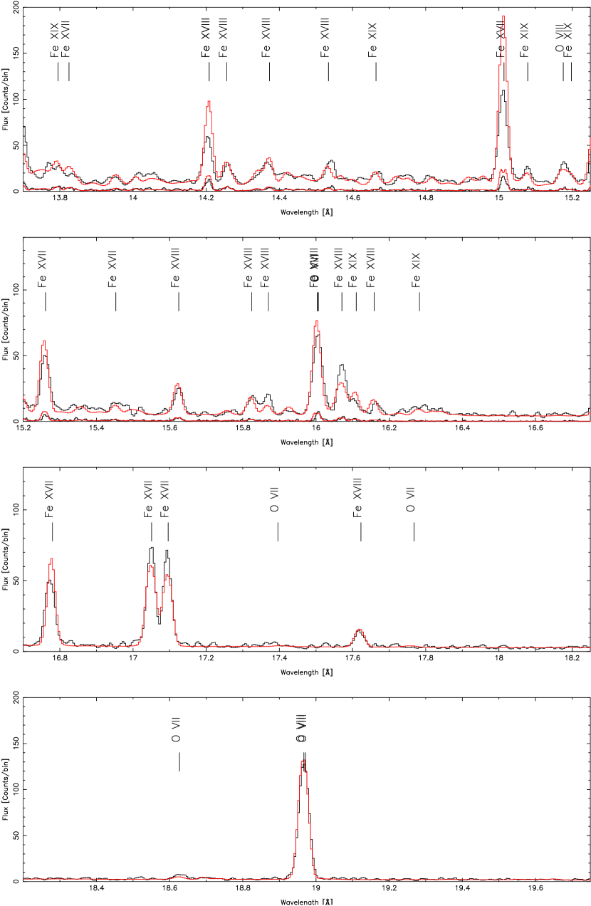
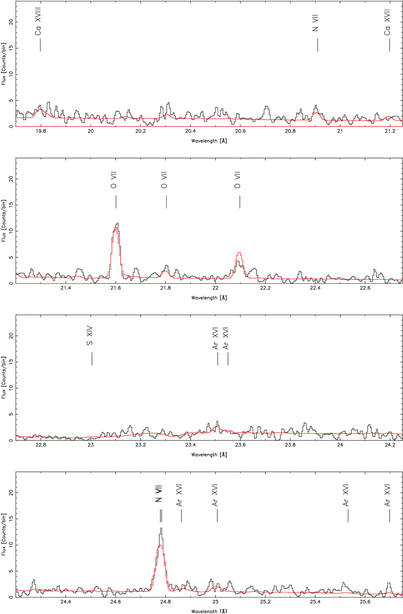
These are the MEG and HEG counts spectra and the folded DEM and abundance model for the summed and orders. Both data and model have been smoothed by a Gaussian convolution with dispersions of 0.005 Å (MEG) and 0.0025 Å (HEG). The model is plotted with a dashed line (solid red in the electronic edition). The MEG spectrum is usually the upper trace, except near Fe xxv, 1.85 Å, where the HEG has more effective area. HEG has about twice the resolution of MEG. Some model lines expected in each region have been labeled. Some regions of the spectrum are well matched by the model. In others, large mismatches are obvious. The spectra are shown in four parts, a-d, each of which has four panels covering about 1.5 Å. Part a spans 1.7–7.7 Å, part b 7.7–13.7 Å, part c 13.7–19.7, and part d 19.7–25.7 Å.
See 4a
See 4a
See 4a
We show the differential emission measure integrated in bins of size for the DEM fit to combined observations. The solid line is the mean of the 100 Monte-Carlo fits, and the dashed lines are the one standard deviation boundaries. The tail above about was manually adjusted (within the one sigma limits) so that the synthetic spectrum’s short wavelength continuum better matched the data, since this wasn’t well constrained by the fit. The peak at 6.2 is constrained by contemporaneous EUVE data. The range including the hot peak at 7.3 and hotter tail is strongly modulated by flares. The integral over the plotted temperature range yields a volume emission measure of .
The abundances relative to Solar are plotted against their first ionization potential. Results from the current work are marked with squares, and the uncertainties are one standard deviation from the Monte Carlo fit. Results from low-resolution X-ray determinations are also plotted (diamonds and asterisks, with dotted error-bars) as well as the AR Lac photospheric values (triangles) and scaled Solar coronal abundances (dashed line); the symbol legend indicates the first author.
In this figure we compare the normalized flux profiles at quadrature and conjunction phases. Normalization is done within the wavelength band by subtracting the minimum and then dividing by the maximum. The solid line profile is from the conjunction phases when the stars’ line-of-sight velocity difference is zero, the dashed quadrature, and the lowest dash-dot line is the difference. The left panel is from MEG and the right is HEG (at the same wavelength, HEG has twice the resolution of the MEG). Both broadening and shifts are apparent.
In this figure we plot the line flux residuals normalized by their measurement uncertainty (upper graph) and the ratio of measured line flux to model flux (bottom graph). The abscissa is the first moment of the line’s emissivity distribution, rather than the temperature of maximum emissivity. This is a conservative bias for the hydrogen-like ions, since they have a long tail on the high-temperature side they move to slightly higher values than their peak. In the both plots, each ion is denoted by the first character in its element abbreviation with some use of lower-case for duplicate characters (see the legend). While many features lie within of zero, many lie outside two and 3, in excess of what would be expected statistically for Gaussian measurement errors alone. Hence, there is a deficiency in the DEM and abundance model, errors in the atomic data, mis-identified and blended lines, or likely, some combination of these.


.