The Evolution of Inverse Power Law Quintessence at Low Redshift

Abstract

Quintessence models based on a scalar field, $\phi$, with an inverse power law potential display simple tracking behavior at early times, when the quintessence energy density, $\rho_{\phi}$, is sub-dominant. At late times, when $\rho_{\phi}$ becomes comparable to the matter density, $\rho_{m}$, the evolution of $\phi$ diverges from its scaling behavior. We calculate the first order departure of $\phi$ from its tracker solution at low redshift. Our results for the evolution of $\phi$, $\rho_{\phi}$, $\Omega_{\phi}$, and $w$ are surprisingly accurate even down to $z=0$. We find that $w$ and $\Omega_{\phi}$ are related linearly to first order, and derive a semi-analytic expression for $w(z)$ which is accurate to within a few percent. Our analytic techniques are potentially applicable to any quintessence model in which the quintessence component comes to dominate at late times.

I Introduction

A host of observations suggest that the universe is currently dominated by some form of energy with negative pressure flat ; WMAP ; lowM ; SN . Recent observations of Type Ia supernovae SN , which appear fainter than they would if the expansion were decelerating due to matter alone, provide the most direct evidence for a dominant negative pressure component (and the accelerating expansion that accompanies it). In addition, cosmic microwave background observations from WMAP, for example, suggest that the universe is nearly flat ($\Omega_{0}\approx 1$) but contains a sub-critical density of matter $\Omega_{m0}=0.27\pm 0.04$ WMAP . Taken together these findings imply the presence of a large fraction of unclustered “dark energy”.

The most straightforward source of dark energy is a cosmological constant, but the level of fine-tuning necessary to make it a viable candidate is disconcerting. An alternative, dubbed quintessence, is a model of time-varying dark energy based on the behavior of a dynamical, classical scalar field $\phi$. In the simplest quintessence models, $\phi$ is taken to be a minimally-coupled field with potential $V(\phi)$, and pressure, energy density, and equation of state

$$p_{\phi}={1\over 2}\dot{\phi}^{2}-V(\phi),$$ (1)

$$\rho_{\phi}={1\over 2}\dot{\phi}^{2}+V(\phi),$$ (2)

and

$$w=p_{\phi}/\rho_{\phi}.$$ (3)

The behavior of the quintessence field will depend, of course, on the particular choice of $V(\phi)$. One widely-investigated case is the inverse power law potential IPL

$$V(\phi)=\kappa\phi^{-\alpha},$$ (4)

where $\kappa$ is a constant with units of $m^{4+\alpha}$.

These potentials are particularly simple and have several desirable properties. They exhibit tracking behavior, ${\it i.e.},~{}$ a wide range of initial conditions converge to a common solution at late times Tracker ; lowIPL . In addition, inverse power law quintessence remains sufficiently subdominant energetically so that it does not disastrously interfere with known epochs of standard big bang cosmology. Finally, because a fundamental understanding of the nature of dark energy must eventually come from particle physics, it is worth noting that inverse power law potentials can arise naturally from extensions to the standard model (e.g., SUSY QCD SUSYQCD ).

The inverse power law tracker solutions are characterized by an equation of state parameter, $w$, which is approximately constant when the universe is dominated by a background fluid. During the matter-dominated era, for example, when the contribution of the quintessence energy density to the expansion is neglected, $w$ is given by IPL ; Tracker ; lowIPL :

$$w=-{2\over 2+\alpha},$$ (5)

and $\phi$ evolves as

$$\phi\propto t^{2/(2+\alpha)},$$ (6)

corresponding to a density which evolves as

$$\rho_{\phi}\propto t^{-2\alpha/(2+\alpha)}.$$ (7)

These expressions provide an excellent approximation to the behavior of the quintessence field as long as $\rho_{\phi}/\rho_{m}\ll 1$.

At late times, however, when the scalar field itself contributes significantly to the expansion of the universe, the value of $w$ begins to diverge from its tracker value, as do $\phi(t)$ and $\rho_{\phi}(t)$. In this paper, we examine analytically the behavior of the scalar field during the transition from matter to scalar-field domination. It is this late-time evolution which is relevant to supernova Ia observations and other tests of dark energy (see, e.g., Ref. multiObs and references therein). A good analytic approximation to the behavior of $\Omega_{\phi}$ and $w$ at late times would be useful in such calculations. Furthermore, our treatment provides insight into the behavior of the scalar field once it begins to dominate.

A number of observations provide stringent upper limits on $w$. For example, the WMAP results, combined with supernovae observations, HST data, 2dFGRS observations of large scale structure, and Lyman alpha forest data give $w\lesssim-0.78$ at 2 $\sigma$ WMAP , assuming constant $w$, which implies a low value for $\alpha$. Nonetheless, we have attempted to keep our approach as general as possible, treating all values of $\alpha$ in the discussion below.

In the following section, we rederive the inverse power law model solutions for $\phi$, $\rho_{\phi}$, and $w$ during the matter-dominated era. In Section III, we use the first-order perturbations to these background solutions to describe the deviation of the scalar field away from tracking behavior as the universe enters the scalar-field dominated era. In Section IV, we compare our analytical results to those of the numerically-integrated evolution equations. We find that the first-order corrections to the background solutions for $\phi$, $\rho_{\phi}$, $\Omega_{\phi}$, and $w$ characterize their behavior surprisingly well even to the present. In Section V, we discuss some consequences of these results.

II Inverse Power Law Quintessence Evolution in the matter-dominated era

The equation of motion for $\phi$ is

$$\ddot{\phi}+3H\dot{\phi}+{dV(\phi)\over d\phi}=0,$$ (8)

where $H=\dot{a}/a$ is the Hubble parameter and $a=a(t)$ is the scale factor which describes the expansion of the universe as a function of time.

We confine our analysis to $z<30$, so that the contribution of radiation to the expansion can be neglected. Assuming a flat universe containing only matter and quintessence, the Friedmann equation is

$$3H^{2}=\rho_{m}+\rho_{\phi},$$ (9)

in units where $8\pi G=1$, which we will use throughout the paper.

When $\rho_{\phi}$ is neglected in equations (8) and (9), it is easy to integrate these equations directly to derive $\phi(t)$, as was done in Refs. IPL ; Tracker ; lowIPL . However, in deriving a perturbative expansion when $\rho_{\phi}/\rho_{m}$ is small but nonzero, it turns out to be easier to use $a$ as the independent variable, rather than $t$. Further, we would like to express observable quantities such as $w$ and $\Omega_{\phi}$ at late times as functions of redshift, rather than time, which is straightforward when the independent variable is taken to be $a$.

Appealing to equation (2) and equation (9), ${1\over 2}\dot{\phi}^{2}$ can be rewritten as

$${1\over 2}\dot{\phi}^{2}={x\over 1-x}(\rho_{m}+V),$$ (10)

where $V$ implicitly means $V(\phi)$ and

$$x={\rho_{\phi}+p_{\phi}\over 2(\rho_{m}+\rho_{\phi})}={{1\over 2}\dot{\phi}^{2}\over 3H^{2}}={1\over 6}{\Big{(}a{d\phi\over da}\Big{)}}^{2}.$$ (11)

Substituting equation (10) into Eqs. (1), (2), (3), and (9), we can rewrite $\rho_{\phi}$, $w$, and the Friedmann equation as follows:

$$\rho_{\phi}={{x\rho_{m}+V}\over 1-x},$$ (12)

$$w={{x\rho_{m}-V(1-2x)}\over{x\rho_{m}+V}},$$ (13)

and

$$3H^{2}={{\rho_{m}+V}\over 1-x}.$$ (14)

Using the above expressions, equation (8) becomes

$$a^{2}{\phi}^{\prime\prime}+{a{\phi}^{\prime}\over 2}(5-3x)+{3(1-x)\over\rho_{m}+V}\Big{(}{a{\phi}^{\prime}V\over 2}+{dV\over d\phi}\Big{)}=0,$$ (15)

where the prime denotes $d/da$. During the matter-dominated epoch, when $x\ll 1$, equation (15) reduces to

$$a^{2}{\phi}^{\prime\prime}_{(0)}+{5a{\phi}^{\prime}_{(0)}\over 2}+{3\over\rho_{m}}{dV\over d\phi}=0,$$ (16)

where the zero subscript in parentheses denotes the zeroth-order solution, neglecting the contribution of quintessence to the expansion rate. (We use the subscript $``(0)"$ throughout to denote such zeroth-order terms, while the subscript $``0"$ without parentheses is reserved for quantities evaluated at the present day).

For quintessence with an inverse power law potential (equation 4), the solution to equation (16) is

$$\phi_{(0)}=C(\alpha){a}^{{3/(2+\alpha)}}.$$ (17)

In equation (17), the constant C($\alpha$) depends on the value of $\alpha$ and is related to $\kappa$ and the present matter density, $\rho_{m0}$, in the following way

$$\kappa=\rho_{m0}{3(4+\alpha)\over 2\alpha(2+\alpha)^{2}}{C(\alpha)}^{2+\alpha}.$$ (18)

The corresponding zeroth-order solution for $\rho_{\phi}$ is

$$\rho_{\phi(0)}=3\rho_{m0}{{C(\alpha)^{2}}\over{\alpha(2+\alpha)}}{a}^{-{3\alpha/(2+\alpha)}}.$$ (19)

The zeroth-order behavior of the quintessence density parameter is then given by $\Omega_{\phi(0)}=\rho_{\phi(0)}/(\rho_{\phi(0)}+\rho_{m})$. Finally, the equation of state is just a constant in the tracking regime:

$$w_{(0)}=-{2\over 2+\alpha}.$$ (20)

These expressions for $\phi_{(0)}(a)$, $w_{(0)}(a)$, and $\rho_{\phi(0)}(a)$ are, of course, equivalent to the previously-derived time-dependent quantities given in Section I.

III First-Order Perturbation to Inverse Power Law Quintessence Evolution

We define the first-order perturbation to the zeroth-order background field $\phi_{(0)}$ (equation 17) to be $\phi_{(1)}$, where

$$\phi_{(1)}/\phi_{(0)}\sim O(\rho_{\phi(0)}/\rho_{m}).$$ (21)

Then the perturbed field, $\phi$, is, to first order,

$$\widetilde{\phi}=\phi_{(0)}+\phi_{(1)},$$ (22)

where we use a tilde throughout to denote quantities expanded to first order in $\rho_{\phi(0)}/\rho_{m}$. Substituting equation (22) into equation (15) and keeping all terms of order ${\rho_{\phi(0)}/\rho_{m}}$ (note, in particular, that $x\sim O(\rho_{\phi(0)}/\rho_{m})$), we find that $\phi_{(1)}$ obeys

$$a^{2}{\phi_{(1)}^{\prime\prime}}+{a\over 2}(5\phi_{(1)}^{\prime}-3x_{(0)}\phi_{(0)}^{\prime})+{3a\phi_{(0)}^{\prime}V\over 2\rho_{m}}$$

$$-{3\rho_{\phi(0)}\over{(\rho_{m})}^{2}}{dV\over d\phi}+{3\over\rho_{m}}{d^{2}V\over d\phi^{2}}\phi_{(1)}=0,$$ (23)

where $x_{(0)}=(a\phi^{\prime}_{(0)})^{2}/6$.

For our particular choice of potential, equation (23) becomes

$$a^{2}{\phi_{(1)}^{\prime\prime}} + {a\over 2}(5\phi_{(1)}^{\prime}-3x_{(0)}\phi_{(0)}^{\prime})+{27\kappa a^{3}\over 2(2+\alpha)\rho_{m0}{(\phi_{(0)})^{(-1+\alpha)}}}$$ (24)

$$+ {3\alpha(1+\alpha)\kappa a^{3}\phi_{(1)}\over\rho_{m0}{(\phi_{(0)})^{(2+\alpha)}}}=0.$$

The solution to equation (24) is

$$\phi_{(1)}=-{3(6+\alpha)\phi_{(0)}^{3}\over\alpha(2+\alpha)(28+8\alpha+{\alpha}^{2})}.$$ (25)

The corresponding corrections to $\rho_{\phi(0)}$ and $w_{(0)}$ are

$$\rho_{\phi(1)}=x_{(0)}\rho_{\phi(0)}+x_{(1)}\rho_{m}-\alpha{\phi_{(1)}\over\phi_{(0)}}V,$$ (26)

and

$$w_{(1)}=(1-w_{(0)})\Big{(}{\rho_{\phi(1)}\over\rho_{\phi(0)}}+\alpha{\phi_{(1)}\over\phi_{(0)}}\Big{)},$$ (27)

where $x_{(1)}=2x_{(0)}{\phi_{(1)}^{\prime}/\phi_{(0)}^{\prime}}$ is defined via $\widetilde{x}=x_{(0)}+x_{(1)}=a^{2}(\phi^{\prime 2}_{(0)}+2\phi^{\prime}_{(0)}\phi^{\prime}_{(1)})/6$.

In terms of $\phi_{(0)}$ and $\phi_{(1)}$, the first-order perturbations to $\rho_{\phi(0)}$ and $w_{(0)}$ are

$$\rho_{\phi(1)}=-\frac{\alpha(4+\alpha)}{6+\alpha}\Big{(}{\phi_{(1)}\over\phi_{(0)}}\Big{)}\rho_{\phi(0)},$$ (28)

and

$$w_{(1)}=-\frac{\alpha(4+\alpha)}{6+\alpha}\Big{(}{\phi_{(1)}\over\phi_{(0)}}\Big{)}w_{(0)}.$$ (29)

Because $\phi_{(1)}$ is negative, equation (28) and equation (29) predict that $\rho_{\phi(1)}$ is positive and $w_{(1)}$ is negative, as expected. Note also that $w_{(1)}/w_{(0)}=\rho_{\phi(1)}/\rho_{\phi(0)}=p_{\phi(1)}/2p_{\phi(0)}$.

Combining the zeroth-order and first-order solutions for $\phi$, $\rho_{\phi}$, and $w$, we get

$$\widetilde{\phi} = \phi_{(0)}+\phi_{(1)},$$

$$= \phi_{(0)}-{3(6+\alpha)\over\alpha(2+\alpha)(28+8\alpha+\alpha^{2})}\phi_{(0)}^{3},$$

$$= \phi_{(0)}\Big{(}1-{3(6+\alpha)\over\alpha(2+\alpha)(28+8\alpha+\alpha^{2})}C(\alpha)^{2}a^{6/(2+\alpha)}\Big{)},$$

$$\widetilde{\rho}_{\phi} = \rho_{\phi(0)}+\rho_{\phi(1)},$$

$$= \rho_{\phi(0)}\Big{(}1-\frac{\alpha(4+\alpha)}{6+\alpha}\Big{(}{\phi_{(1)}\over\phi_{(0)}}\Big{)}\Big{)},$$

$$= \rho_{\phi(0)}\Big{(}1+{3(4+\alpha)\over(2+\alpha)(28+8\alpha+\alpha^{2})}C(\alpha)^{2}a^{6/(2+\alpha)}\Big{)},$$

and

$$\widetilde{w} = w_{(0)}+w_{(1)},$$

$$= w_{(0)}\Big{(}1-\frac{\alpha(4+\alpha)}{6+\alpha}\Big{(}{\phi_{(1)}\over\phi_{(0)}}\Big{)}\Big{)},$$

$$= w_{(0)}\Big{(}1+{3(4+\alpha)\over(2+\alpha)(28+8\alpha+\alpha^{2})}C(\alpha)^{2}a^{6/(2+\alpha)}\Big{)}.$$

We also define $\widetilde{\Omega}_{\phi}=\widetilde{\rho}_{\phi}/(\widetilde{\rho}_{\phi}+\rho_{m})$.

IV A comparison of Analytic and Numerical Results

To test the accuracy of our analytical predictions, we numerically integrate equation (8) for the cases $\alpha=1$, $\alpha=2$, and $\alpha=4$. In order to compare analytic and numerical results for a specific case, we adjust $\kappa$ to give $\Omega_{m0}=0.3$ and $\Omega_{\phi 0}=0.7$. In figures $1-4$ below, the zeroth-order (tracker) and first-order analytic solutions for $\phi$, $\rho_{\phi}$, $\Omega_{\phi}$, and $w$ are compared to their numerical counterparts.

In Fig. 1, we present the ratios of the tracker and first-order quintessence fields to the true (numerical) field: $\phi_{(0)}/\phi$, and $\widetilde{\phi}/\phi$, respectively. As expected, $\widetilde{\phi}$ agrees exceptionally well with the true evolution at early times, when the quintessence density is sub-dominant; the error for all three cases is less than 2% for $z\geq 1$. The analytic expression begins to break down at later times, becoming significantly less accurate at $z=0$, but it is still much more representative of the true behavior than the tracker solution $\phi_{(0)}$.

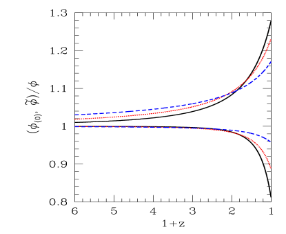
Figure 1: The ratios $\phi_{(0)}/\phi$ (upper three curves) and $\widetilde{\phi}/\phi$ (lower three curves) for $\alpha=1$ (black, solid), $\alpha=2$ (red, dotted), and $\alpha=4$ (blue, dashed).

In Fig. 2, we present $\rho_{\phi(0)}/\rho_{\phi}$, and $\widetilde{\rho}_{\phi}/\rho_{\phi}$.

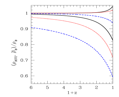
Figure 2: The ratios $\rho_{\phi(0)}/\rho_{\phi}$ (lower three curves) and $\widetilde{\rho}_{\phi}/\rho_{\phi}$ (upper three curves) for $\alpha=1$ (black, solid), $\alpha=2$ (red, dotted), and $\alpha=4$ (blue, dashed).

Here the power of the first-order approach is evident. The first-order solutions in these cases are accurate to within 6% all of the way down to $z=0$. In contrast, the tracker expression for $\rho_{\phi}$ grossly underestimates the quintessence density at low redshift.

In Fig. 3, we give the ratios $\Omega_{\phi(0)}/\Omega_{\phi}$ and $\widetilde{\Omega}_{\phi}/\Omega_{\phi}$.

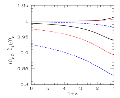
Figure 3: The ratios $\Omega_{\phi(0)}/\Omega_{\phi}$ (lower three curves) and $\widetilde{\Omega}_{\phi}/\Omega_{\phi}$ (upper three curves) for $\alpha=1$ (black, solid), $\alpha=2$ (red, dotted), and $\alpha=4$ (blue, dashed).

The agreement between $\widetilde{\Omega}_{\phi}$ and the true $\Omega_{\phi}$ is quite remarkable. Down to $z=1$, the error in the first-order expression is less than 1% for all three cases we have examined, and even at $z=0$, the error is less than 2%.

Finally, we consider the equation of state parameter, $w$. In Fig. 4, we show the ratio of the tracker value $w_{(0)}$ (which is, of course, constant) to the true $w$ and $\widetilde{w}/w$.

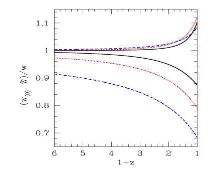
Figure 4: The ratios $w_{(0)}/w$ (lower three curves) and $\widetilde{w}/w$ (upper three curves) for $\alpha=1$ (black, solid), $\alpha=2$ (red, dotted), and $\alpha=4$ (blue, dashed).

Agreement between $\widetilde{w}$ and $w$ is quite good at early times, with an error of less than 2% for $z\geq 1$, increasing to 4% at $z=0.5$ and 10% at $z=0$.

V Discussion

Our first-order corrections to the pure matter-dominated solutions for $\phi$, $\rho_{\phi}$, $\Omega_{\phi}$, and $w$ characterize the evolution of these quantities extremely well at $1+z>2$. Although, unsurprisingly, the first-order solutions begin to break down for $1+z<2$, when the quintessence component dominates the expansion, they are suprisingly accurate even to the present.

We can draw some simple qualititative conclusions from these results. It is instructive to use equations (19) and (III) to express ${w}$ as a function of $\Omega_{\phi}$, since these are the two directly-observable quantities of interest. We find, to first order in $\rho_{\phi(0)}/\rho_{m}$:

$${w}=-{2\over 2+\alpha}-{2\alpha(4+\alpha)\over(2+\alpha)(28+8\alpha+\alpha^{2})}\Omega_{\phi}.$$ (33)

The first term in this equation is just $w_{(0)}$, while the second term shows how ${w}$ diverges from the tracker value at early times, when the quintessence field is just starting to contribute to the expansion of the universe. We see that the deviation of ${w}$ from $w_{(0)}$ depends linearly on $\Omega_{\phi}$. Further, the constant of proportionality is a slowly-varying function of $\alpha$, ranging from 0.09 for $\alpha=1$ to 0.14 for $\alpha=4$. Hence, the rate at which $w$ deviates from $w_{(0)}$ at early times is almost independent of $\alpha$. Equation (33) is an excellent fit for small $\Omega_{\phi}$, but it works suprisingly well even up to the present. For $\alpha=1-4$, the error in the prediction for $w$ is less than 10%, with smaller errors for smaller (and more physically relevant) values of $\alpha$.

A number of approximations have been proposed to simulate the evolution of $w$ at late times. For arbitrary quintessence models, a common approximation is a Taylor expansion in $z$ astier ; goliath ; maor ; huterer ; weller :

$$w_{\rm lin}=w_{0}+w_{1}z+...,$$ (34)

while more complex parametrizations have been examined by Bassett et al.bassett and by Corasaniti and Copeland corasaniti .

For the specific case of inverse power-law models, Efstathiou GE showed that a good empirical fit to the time-evolution of $w$ is:

$$w_{\rm Efst}=w_{0}+w_{1}\ln(1+z).$$ (35)

Our results suggest an alternative parametrization. We can write equation (III) in the form

$$w_{\rm fit}=w_{(0)}+(w_{0}-w_{(0)})(1+z)^{-6/(2+\alpha)},$$ (36)

Since $w_{(0)}$ is given by equation (20), equation (36) has only one undetermined parameter, the present value of the equation of state, $w_{0}$, which can be determined numerically and used to derive a fit to $w$. As shown in Fig. 5, the error introduced by this

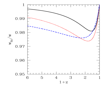
Figure 5: The ratio $w_{\rm fit}/w$, where $w_{\rm fit}$ is given by equation (36), for $\alpha=1$ (black, solid), $\alpha=2$ (red, dotted), and $\alpha=4$ (blue, dashed).

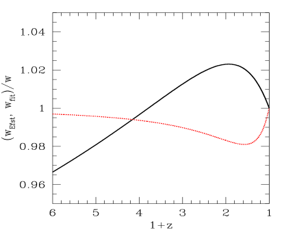
Figure 6: The ratios $w_{\rm Efst}/w$ (black, solid), and $w_{\rm fit}/w$ (red, dotted) for the $\alpha=1$ case.

approximation is less than 3% for $\alpha$ in the range $1-4$.

To show how our fit (equation 36) compares to the empirical fit of equation (35), we have plotted their behavior for the $\alpha=1$ case in Fig. 6. A $\chi^{2}$ minimization routine was used to determine the best-fit value of $w_{1}$ over the plotted redshift range for $w_{\rm Efst}$. (In both approximations, we set $w_{0}$ equal to the present-day value of the equation of state that is found numerically for $\alpha=1$). Despite the fact that $w_{\rm Efst}$ contains one more fitted parameter than $w_{\rm fit}$, it is clear from Fig. 6 that $w_{\rm fit}$ agrees better with the numerical behavior of $w$ at high redshift and shows comparable accuracy at low redshift. Note, however, that if we restrict the redshift range to much lower $z$ (e.g., $0<z<1$), and recalculate $w_{1}$ to give the best fit for $w_{\rm Efst}$ only within this redshift range, then $w_{\rm Efst}$ gives better agreement than $w_{\rm fit}$, although both expressions are accurate to within 2% over this redshift interval.

Neither of these results is unexpected. The expression for $w_{\rm fit}$ in equation (36) is derived by perturbing the high-redshift evolution of $\phi$, so we expect it to be more accurate at higher redshifts than $w_{\rm Efst}$. On the other hand, the expression for $w_{\rm Efst}$ was derived from an empirical fit at low $z$, and so it is no surprise that this expression can be made to work better at low redshifts.

While we have tested our results against a fiducial flat model with $\Omega_{m0}=0.3$, nothing in our analysis depends on this assumption. For obvious reasons, the agreement between our analytic results and the true evolution of $\rho_{\phi}$ and $w$ will be better than the ones presented here if $\Omega_{m0}>0.3$, and worse if $\Omega_{m0}<0.3$.

Although we have concentrated specifically on the inverse power-law potentials in this paper, it is obvious that the techniques exploited here can be applied to any quintessence model in which the quintessence energy density is subdominant at early times and dominates at low redshift.

VI Acknowledgments

R.J.S. was supported in part by the Department of Energy (DE-FG02-91ER40690).

References

- (1) M. Kamionkowski, et al., Astrophys. J. 426, L57 (1994)
- (2) D. N. Spergel et al., Astrophys. J. , in press, astro-ph/0302207.
- (3) N. A. Bahcall, J. P. Ostriker, S. Perlmutter and P. J. Steinhardt, Science 284, 1481 (1999); L. Verde et al. Mon. Not. R. Astron. Soc. 335, 432 (2002).
- (4) A. G. Riess, et al., AJ 116, 1009 (1998); S. Perlmutter, et al., ApJ 517, 565 (1999).
- (5) P. J. E. Peebles and B. Ratra, Astrophys. J. 325, L17 (1988); B. Ratra and P. J. E. Peebles, Phys. Rev. D 37, 3406 (1988).
- (6) I. Zlatev, L. Wang, and P. J. Steinhardt, Phys. Rev. Lett. 82, 896 (1999); P. J. Steinhardt, L. Wang, and I. Zlatev, Phys. Rev. D 59, 123504 (1999).
- (7) A. R. Liddle and R. J. Scherrer, Phys. Rev. D 59, 023509 (1999).
- (8) P. Binétruy, Phys. Rev. D 60, 063502 (1999); A. Masiero, M. Pietroni and F. Rosati, Phys. Rev. D 61, 023504 (2000).
- (9) J. Kujat, A. Linn, R. J. Scherrer, D. Weinberg, Astrophys. J. 572, 1 (2002)
- (10) P. Astier, Phys. Lett. B 500, 8 (2001).
- (11) M. Goliath, R. Amanullah, P. Astier, A. Goobar, and R. Pain, Astron. Astrophys. 380, 6 (2001).
- (12) I. Maor, R. Brustein, and P.J. Steinhardt, Phys. Rev. Lett. 86, 6 (2001).
- (13) D. Huterer and M.S. Turner, Phys. Rev. D. 64, 123527 (2001).
- (14) J. Weller and A. Albrecht, Phys. Rev. Lett. 86, 1939 (2001).
- (15) B.A. Bassett, M. Kunz, J. Silk, and C. Ungarelli, Mon. Not. R. Astron. Soc. 336, 1217 (2002).
- (16) P.S. Corasaniti and E.J. Copeland, Phys. Rev. D 67, 063521 (2003).
- (17) G. Efstathiou, Mon. Not. R. Astron. Soc. 310, 842 (1999).