Ballooning Modes in Thin Accretion Disks:
Limits for their Excitation

Abstract

The conditions that limit the possible excitation of ideal MHD axisymmetric ballooning modes in thin accretion disks are discussed. As shown earlier by Coppi & Coppi (2001a), these modes are well-localized in the vertical direction but have characteristic oscillatory and non-localized profiles in the radial direction. A necessary condition for their excitation is that the magnetic energy be considerably lower than the thermal energy. Even when this is satisfied, there remains the problem of identifying the possible physical factors which can make the considered modes radially localized. The general solution of the normal mode equation describing the modes is given, showing that it is characterized by a discrete spectrum of eigensolutions. The growth rates are reduced and have a different scaling relative to those of the “long-cylinder” modes, commonly known as the Magneto Rotational Instability, that have been previously studied.

1 Introduction

The problem of identifying the processes which can produce significant transport of angular momentum outward in accretion disks has led to consider the plasma collective modes that can be excited in rotating plasmas where a magnetic field is present. In these plasmas the angular momentum is assumed to increase with the distance from the axis of rotation as in the case of Keplerian accretion disks. The most immediate approach to this problem is that of considering modes that are axisymmetric and are of the same type as those found originally for a long cylindrical plasma (Velikhov, 1959; Chandrasekhar, 1960; Balbus & Hawley, 1991).

Coppi & Coppi (2001a, b) pointed out that these axisymmetric modes when applied to a thin disk configuration become of the ballooning type (Coppi, 1977) in the vertical direction, i.e. they cannot be represented by a single Fourier harmonic, and acquire a characteristic oscillation in the radial direction. The radial wavelength is related to the distance over which the mode is localized vertically. Thus the problem of finding a localizing factor in the radial direction for the axisymmetric modes was left unresolved. As pointed out by Coppi & Coppi (2001c) the scaling of the growth rates of these ballooning modes is different from that of the original modes, which are appropriate for a long cylinder rather than for a thin disk, and are reduced by the condition of vertical localization.

In the present paper we discuss the general solution of the two-dimensional equation that describes the axisymmetric modes in thin plasma disks where the magnetic energy density is much smaller than the thermal energy density. Two categories of modes are identified: the localized ballooning modes that have a discrete spectrum and the quasi-localized modes that have a continuous spectrum of growth rates and related radial wavelenths. These quasi-localized modes can be considered to be physically significant (i.e. to be sufficiently well-localized vertically) only for very large values of $\beta^{t}_{s}\equiv c_{s}^{2}/v_{\scriptscriptstyle A}^{2}$ where $c_{s}$ is the sound velocity and $v_{\scriptscriptstyle A}$ the Alfvén velocity. As is well known, the ratio $H/R$ is of the order of $c_{s}/v_{\scriptscriptstyle\phi}$ where $v_{\scriptscriptstyle\phi}=\Omega R$ and $\Omega=\Omega(R)$ is the local rotation frequency.

When all the limitations are considered, even if a factor providing a radial localization for this kind of mode has not been identified yet, the rate of angular momentum transport that can be expected from its excitation does not appear to have the magnitude of those semi-empirical forms of the diffusion coefficients for the angular momentum transport that are used in current models of disks.

In Section 2 the set of two-dimensional equations that give the spatial profile of axisymmetric modes is derived pointing out all the limits of the derivation. In Section 3 the vertical profile of the mode is shown to be described by a fourth order differential equation under realistic conditions.

In Section 4, we give different analytical derivations of the localized solutions of this mode equation, corresponding to a discrete spectrum of growth rates and of radial wave numbers, in order to better describe the properties and the limitations of these solutions. The asymptotic decay of the modes in the vertical direction is proportional to a Gaussian.

In Section 5 we introduce the class of “quasi-localized” modes whose asymptotic decay in the vertical direction is not proportional to a Gaussian but is algebraic and that have a continuous spectrum.

In Section 6 the issue of the mode radial localization is discussed and the difficulty of constructing mode packets that could be radially localized is pointed out. We compare the ballooning modes to non-normal mode packets which may be formed from MRI modes to achieve vertical localization. And finally the rate of angular momentum transport that can be expected from these modes is estimated and compared to that corresponding to currently adopted effective diffusion coefficients.

2 Mode Profile Equation

We adopt cylindrical coordinates and note that axisymmetric modes are represented by the perturbed toroidal velocity

$$\hat{v}_{\scriptscriptstyle\phi}=\;{\stackrel{{\scriptstyle\scriptscriptstyle\approx}}{{v}}_{\scriptscriptstyle\phi}\!(R,z)}\;\exp(\gamma_{\scriptscriptstyle 0}t)\;.$$

In order to identify the properties of ${\stackrel{{\scriptstyle\scriptscriptstyle\approx}}{{v}}_{\scriptscriptstyle\phi}\!(R,z)}$ we start by writing the total momentum conservation equation as

$$\hat{\mathbf{A}}_{m}\equiv\rho\left(\frac{\partial}{\partial t}\hat{\mathbf{v}}+\mathbf{v}\cdot\nabla\hat{\mathbf{v}}+\hat{\mathbf{v}}\cdot\nabla\mathbf{v}\right)+\nabla\left(\hat{p}+\frac{1}{4\pi}\mathbf{B}\cdot\hat{\mathbf{B}}\right)-\frac{1}{4\pi}\mathbf{B}\cdot\nabla\hat{\mathbf{B}}\simeq 0$$ (1)

where we neglect the $R$ derivatives of all equilibrium quantities when compared to the $R$ derivatives of the perturbation. Then, as is customary in the theory of ideal MHD modes, we consider the $\mathbf{e}_{\phi}\cdot\nabla\times\hat{\mathbf{A}}_{m}=0$ component of Eq. (1). This is

$$\frac{\partial}{\partial z}\hat{A}_{mR}-\frac{\partial}{\partial R}\hat{A}_{mz}=0$$

and, specifically,

$$\frac{\partial}{\partial z}\left[\rho\left(\gamma_{\scriptscriptstyle 0}\hat{v}_{\scriptscriptstyle R}-2\Omega\hat{v}_{\scriptscriptstyle\phi}\right)-\frac{1}{4\pi}B_{z}\frac{\partial}{\partial z}\hat{B}_{\scriptscriptstyle R}\right]-\frac{\partial}{\partial R}\left[\gamma_{\scriptscriptstyle 0}\rho\hat{v}_{z}-\frac{1}{4\pi}B_{z}\frac{\partial}{\partial z}\hat{B}_{z}\right]=0$$ (2)

We note that, as shown by Coppi & Coppi (2001a, b), $\hat{v}_{\scriptscriptstyle\phi}$ and the plasma displacement $\tilde{\xi}_{\scriptscriptstyle R}$ do not vanish when $\gamma_{\scriptscriptstyle 0}/\Omega\rightarrow 0$, while $\hat{v}_{\scriptscriptstyle R}=\gamma_{\scriptscriptstyle 0}\hat{\xi}_{\scriptscriptstyle R}$, $\hat{v}_{z}=\gamma_{\scriptscriptstyle 0}\hat{\xi}_{z}$, and the compressibility

$$\nabla\cdot\mathbf{v}\simeq\gamma_{\scriptscriptstyle 0}\left(\frac{\partial}{\partial R}\hat{\xi}_{\scriptscriptstyle R}+\frac{\partial}{\partial z}\hat{\xi}_{z}\right)\simeq\gamma_{\scriptscriptstyle 0}\nabla\cdot\hat{\xi}$$

do. For the modes of interest the variation of ${\stackrel{{\scriptstyle\scriptscriptstyle\approx}}{{v}}_{\scriptscriptstyle\phi}\!(R,z)}$ on $z$ occurs on a scale distance that is considerably shorter than that for the variation of $B_{z}$. This is consistent with the fact that, in the considered region, the $B_{\scriptscriptstyle R}$ component of the field is negligible.

The frozen-in law can be written in the form

$$\frac{\partial\hat{\mathbf{B}}}{\partial t}=\left(\mathbf{B}\cdot\nabla\hat{\mathbf{v}}+\hat{\mathbf{B}}\cdot\nabla\mathbf{v}\right)-\mathbf{B}\left(\nabla\cdot\hat{\mathbf{v}}\right)-\left(\hat{\mathbf{v}}\cdot\nabla\mathbf{B}+\mathbf{v}\cdot\nabla\hat{\mathbf{B}}\right)$$ (3)

and the $R$ component of it yields

$$\hat{B}_{\scriptscriptstyle R}=B_{z}\frac{\partial}{\partial z}\hat{\xi}_{\scriptscriptstyle R}$$

$$\frac{\partial}{\partial z}\hat{B}_{z}\simeq-\frac{\partial}{\partial R}\hat{B}_{\scriptscriptstyle R}\simeq-B_{z}\frac{\partial}{\partial R}\frac{\partial}{\partial z}\hat{\xi}_{\scriptscriptstyle R}\;.$$

Thus Eq. (2) becomes

$$\frac{\partial^{2}}{\partial z^{2}}\left[\rho\left(\gamma_{\scriptscriptstyle 0}^{2}\hat{\xi}_{\scriptscriptstyle R}-2\Omega\hat{v}_{\scriptscriptstyle\phi}\right)-\frac{1}{4\pi}B_{z}^{2}\frac{\partial^{2}}{\partial z^{2}}\hat{\xi}_{\scriptscriptstyle R}\right]-\frac{\partial^{2}}{\partial R^{2}}\left[-\gamma_{\scriptscriptstyle 0}^{2}\rho\hat{\xi}_{\scriptscriptstyle R}+\frac{1}{4\pi}B_{z}^{2}\frac{\partial^{2}}{\partial z^{2}}\hat{\xi}_{\scriptscriptstyle R}\right]-\gamma_{\scriptscriptstyle 0}^{2}\rho\frac{\partial}{\partial R}\nabla\cdot\hat{\xi}\simeq 0\;.$$ (4)

Now, we write

$$\hat{v}_{\scriptscriptstyle\phi}\equiv-\frac{d\Omega}{dR}R\hat{\xi}_{\scriptscriptstyle R}+\gamma_{\scriptscriptstyle 0}\hat{\xi}_{\scriptscriptstyle\phi}$$

considering the fact that for $\gamma_{\scriptscriptstyle 0}=0$ the frozen-in law (3) gives $\hat{v}_{\scriptscriptstyle\phi}=-(d\Omega/dR)R\hat{\xi}_{\scriptscriptstyle R}$. Then the $\phi$ component of Eq. (3) gives

$$\hat{B}_{\scriptscriptstyle\phi}=B_{z}\frac{\partial}{\partial z}\hat{\xi}_{\scriptscriptstyle\phi}-B_{\scriptscriptstyle\phi}\nabla\cdot\hat{\xi}$$

and the $\phi$ component of Eq. (1) becomes

$$\rho\gamma_{\scriptscriptstyle 0}\left(\gamma_{\scriptscriptstyle 0}\hat{\xi}_{\scriptscriptstyle\phi}+2\Omega\hat{\xi}_{\scriptscriptstyle R}\right)\simeq\frac{1}{4\pi}B_{z}\frac{\partial}{\partial z}\left(B_{z}\frac{\partial}{\partial z}\hat{\xi}_{\scriptscriptstyle\phi}-B_{\scriptscriptstyle\phi}\nabla\cdot\hat{\xi}\right)\;.$$ (5)

Now the set of equations (4) and (5) needs to be completed by one that would relate $\nabla\cdot\hat{\xi}$ to $\hat{\xi}_{\scriptscriptstyle R}$ and $\hat{\xi}_{\scriptscriptstyle\phi}$. Therefore we note that the adiabatic equation of state gives

$$\hat{p}\simeq-p\Gamma\left(\nabla\cdot\hat{\xi}\right)$$

and that by neglecting the $z$ derivatives of the equilibrium quantities relative to those of the perturbations in the equation $\partial\hat{A}_{mz}/\partial z=0$ we obtain, for $\partial\hat{\xi}_{z}/\partial z=\nabla\cdot\hat{\xi}-\partial\hat{\xi}_{\scriptscriptstyle R}/\partial R$,

$$\gamma_{\scriptscriptstyle 0}^{2}\left(\nabla\cdot\hat{\xi}-\frac{\partial}{\partial R}\hat{\xi}_{\scriptscriptstyle R}\right)+\frac{\partial^{2}}{\partial z^{2}}\left[v_{{\scriptscriptstyle A}{\scriptscriptstyle\phi}}^{2}\frac{\hat{B}_{\scriptscriptstyle\phi}}{B_{\scriptscriptstyle\phi}}-c_{s}^{2}\left(\nabla\cdot\hat{\xi}\right)\right]\simeq 0$$ (6)

with $\Gamma=5/3$ and $c_{s}^{2}\equiv\Gamma p/\rho$.

Since, as will be shown in the following analysis, the excitation of axisymmetric modes is possible only if $v_{{\scriptscriptstyle A}{\scriptscriptstyle\phi}}^{2}\ll c_{s}^{2}$, we consider regimes for which this is the case and $\gamma_{\scriptscriptstyle 0}^{2}\ll c_{s}^{2}|\partial^{2}/\partial z^{2}|$. Then Eq. (6) reduces to

$$\frac{\partial^{2}}{\partial z^{2}}\left(\nabla\cdot\hat{\xi}\right)\simeq\frac{\gamma_{\scriptscriptstyle 0}^{2}}{c_{s}^{2}}\frac{\partial}{\partial R}\hat{\xi}_{\scriptscriptstyle R}+\frac{v_{{\scriptscriptstyle A}z}^{2}}{c_{s}^{2}}\frac{B_{\scriptscriptstyle\phi}}{B_{z}}\frac{\partial^{3}}{\partial z^{3}}\hat{\xi}_{\scriptscriptstyle\phi}$$ (7)

This indicates that the terms involving $\nabla\cdot\hat{\xi}$ can be neglected in Eqs. (4) and (5) and the set of equations that describe the axisymmetric modes reduces to

$$\rho\gamma_{\scriptscriptstyle 0}\left(\gamma_{\scriptscriptstyle 0}\hat{\xi}_{\scriptscriptstyle\phi}+2\Omega\hat{\xi}_{\scriptscriptstyle R}\right)=\frac{1}{4\pi}B_{z}^{2}\frac{\partial^{2}}{\partial z^{2}}\hat{\xi}_{\scriptscriptstyle\phi}$$ (8)

and

$$\frac{\partial^{2}}{\partial z^{2}}\left[\rho\left(\gamma_{\scriptscriptstyle 0}^{2}\hat{\xi}_{\scriptscriptstyle R}-2\Omega\gamma_{\scriptscriptstyle 0}\hat{\xi}_{\scriptscriptstyle\phi}+2\Omega\Omega^{\prime}R\hat{\xi}_{\scriptscriptstyle R}\right)-\frac{1}{4\pi}B_{z}^{2}\left(\frac{\partial^{2}}{\partial z^{2}}+\frac{\partial^{2}}{\partial R^{2}}\right)\hat{\xi}_{\scriptscriptstyle R}\right]+\frac{\partial^{2}}{\partial R^{2}}\left(\gamma_{\scriptscriptstyle 0}^{2}\rho\hat{\xi}_{\scriptscriptstyle R}\right)=0\;.$$ (9)

In order to assess the influence of the modes that can be excited on the effective rate of transport of angular moment in thin accretion disks, a number of factors have to be considered. Thus the most evident factors to be taken into account in looking for the possible solutions of Eqs. (8) and (9) are:

• The mode growth rate

• The vertical and radial characteristic scale distances

• The value of the threshold for the mode onset

• Whether or not a mode is contained (localized) vertically within the disk and whether appropriate non-normal modes (packets) can be constructed

• The physical features that may localize the mode radially.

In particular, it is well known that the rate of transport which can be produced by excited plasma modes can be assessed in a rudimentary way from an effective diffusion coefficient that includes both the mode growth rate and its characteristic wavelenths. Therefore modes with very short wavelengths may be less effective that modes with longer wavelengths even if the growth rates of the latter modes are smaller.

For the sake of simplicity, we do not consider at first the condition that a mode should be vertically localized within a disk nor the criterion that it should have the lowest threshold $\Omega_{c}$ possible for its onset ($\Omega>\Omega_{c}$). In particular, we refer to modes that are propagating in the vertical direction, have vertical wavelenths $\lambda_{z}=2\pi/k_{z}$ that are much smaller than the height of the disk, $2H$, and involve the central value of the particle density $\rho_{\scriptscriptstyle 0}\equiv\rho(z=0)$. We assume also that the modes are propagating radially. Therefore

$${\stackrel{{\scriptstyle\scriptscriptstyle\approx}}{{v}}_{\scriptscriptstyle\phi}\!(R,z)}\simeq\rm\exp\left[ik_{z}z+ik_{\scriptscriptstyle R}\left(R-R_{\scriptscriptstyle 0}\right)\right]$$

where $R=R_{\scriptscriptstyle 0}$ is the radius at which all equilibrium quantities entering Eqs. (8) and (9) are evaluated, and $k_{z}H\gg 1$. Thus Eq. (8) becomes

$$\left(\gamma_{\scriptscriptstyle 0}^{2}+\omega_{{\scriptscriptstyle A}z}^{2}\right)\rm=-\gamma_{\scriptscriptstyle 0}2\Omega\tilde{\xi}_{\scriptscriptstyle R}$$

where $\omega_{{\scriptscriptstyle A}z}^{2}\equiv k_{z}^{2}v_{{\scriptscriptstyle A}z}^{2}$, $v_{{\scriptscriptstyle A}z}^{2}\equiv B_{z}^{2}/(4\pi\rho_{\scriptscriptstyle 0})$, and Eq. (9)

$$\left(\gamma_{\scriptscriptstyle 0}^{2}+\omega_{{\scriptscriptstyle A}z}^{2}\right)k^{2}\tilde{\xi}_{\scriptscriptstyle R}-3\Omega^{2}k_{z}^{2}\tilde{\xi}_{\scriptscriptstyle R}-2\Omega\gamma_{\scriptscriptstyle 0}\rm k_{z}^{2}=0$$

where $k^{2}\equiv k_{\scriptscriptstyle R}^{2}+k_{z}^{2}$ and we have taken $2\Omega^{\prime}\Omega R=-3\Omega^{2}$ as appropriate for a Keplerian disk. The resulting dispersion relation is

$$\gamma_{\scriptscriptstyle 0}^{4}+\gamma_{\scriptscriptstyle 0}^{2}\left(2\omega_{{\scriptscriptstyle A}z}^{2}+\Omega^{2}\frac{k_{z}^{2}}{k^{2}}\right)=\omega_{{\scriptscriptstyle A}z}^{2}\left(3\Omega^{2}\frac{k_{z}^{2}}{k^{2}}-\omega_{{\scriptscriptstyle A}z}^{2}\right)\;.$$ (10)

We see that the instability threshold is $3\Omega^{2}=k^{2}v_{{\scriptscriptstyle A}z}^{2}$, implying very high values of $\beta_{s}\equiv c_{s}^{2}/v_{{\scriptscriptstyle A}z}^{2}$ as $k^{2}>k_{z}^{2}\gg 1/H^{2}$, and that the maximum growth rate ($\gamma_{\scriptscriptstyle 0}$ relatively close to $\Omega$) is found for $k_{\scriptscriptstyle R}^{2}\ll k_{z}^{2}$. This is the limit in which the Velikhov (a.k.a. MRI) instability is found. The question then arises whether the assumptions that have to be made to arrive at Eq. (10) can make these types of modes good candidates to produce the needed rate of transport in thin accretion disks. Therefore, in the next section we look for the modes that can be contained in the disk vertically and have the lowest threshold possible.

3 Contained Modes

Now we analyze the characteristics of the modes that are localized near the center of the disk over a distance smaller than $H$ where the density $\rho(z)$ can be approximated by

$$\rho\simeq\rho_{\scriptscriptstyle 0}\left(1-\frac{z^{2}}{H_{\scriptscriptstyle 0}^{2}}\right)$$ (11)

and $H\sim H_{\scriptscriptstyle 0}$.

These modes, as was demonstrated by Coppi & Coppi (2001a, b), are characterized by being evanescent in the vertical direction and oscillatory in the radial direction and are represented by

$${\stackrel{{\scriptstyle\scriptscriptstyle\approx}}{{\xi}}_{\scriptscriptstyle R}(R,z)}\simeq\tilde{\xi}_{\scriptscriptstyle R}(z)\exp\left[-ik_{\scriptscriptstyle R}\left(R-R_{\scriptscriptstyle 0}\right)\right]$$

where $\tilde{\xi}_{\scriptscriptstyle R}(z)$ is an even or odd function of $z$ such that $\tilde{\xi}_{\scriptscriptstyle R}(|z|\rightarrow H)\rightarrow 0$. Two other important points are that, contrary to the case where Velikhov modes with the highest growth rates can be found,

$$k_{\scriptscriptstyle R}^{2}>\left|\frac{1}{\tilde{\xi}_{\scriptscriptstyle R}}\frac{\partial^{2}}{\partial z^{2}}\tilde{\xi}_{\scriptscriptstyle R}\right|$$

and the relevant growth rates (Coppi & Coppi, 2001c) scale as

$$\gamma_{\scriptscriptstyle 0}^{2}\sim\frac{v_{{\scriptscriptstyle A}z}^{2}}{H_{\scriptscriptstyle 0}^{2}}<\Omega^{2}\;.$$ (12)

Therefore axisymmetric modes that are contained within the disk have a characteristic growth rate that depends on the scale height of the disk and is well below that of the MRI instability.

We note that, as shown by Eq. (7), $|\nabla\cdot\hat{\xi}|\ll|\partial\tilde{\xi}_{\scriptscriptstyle R}/\partial R|$. Therefore $ik_{\scriptscriptstyle R}\tilde{\xi}_{\scriptscriptstyle R}\simeq-d\tilde{\xi}_{z}/dz$,

$$\tilde{\xi}_{z}(z)\simeq ik_{\scriptscriptstyle R}\int\limits_{-\infty}^{z}\tilde{\xi}_{\scriptscriptstyle R}(z^{\prime})dz^{\prime}\;,$$ (13)

and $\tilde{\xi}_{z}(z)$ has the opposite parity of $\tilde{\xi}_{\scriptscriptstyle R}(z)$. Moreover, since $\tilde{\xi}_{z}(z)$ has to be localized, like $\tilde{\xi}_{\scriptscriptstyle R}(z)$, within the disk the solution $\tilde{\xi}_{\scriptscriptstyle R}(z)$ is subject to the condition

$$\int\limits_{-\infty}^{+\infty}\tilde{\xi}_{\scriptscriptstyle R}(z^{\prime})dz^{\prime}=0\;.$$ (14)

The problem to be solved is simplified if we note that Eq. (8) reduces to

$$2\Omega\gamma_{\scriptscriptstyle 0}\tilde{\xi}_{\scriptscriptstyle R}\simeq v_{{\scriptscriptstyle A}z}^{2}\frac{d^{2}}{dz^{2}}\rm$$ (15)

by observing that $\gamma_{\scriptscriptstyle 0}^{2}\sim v_{{\scriptscriptstyle A}z}^{2}/H_{\scriptscriptstyle 0}^{2}$ and that the modes we look for are localized within $-H_{\scriptscriptstyle 0}<z<H_{\scriptscriptstyle 0}$:

$$H_{\scriptscriptstyle 0}^{2}\left|\frac{1}{\rm}\frac{d^{2}}{dz^{2}}\rm\right|^{2}\gg 1\;.$$

Under the same conditions Eq. (9) reduces to

$$\frac{d^{2}}{dz^{2}}\left[\left(k_{\scriptscriptstyle R}^{2}v_{{\scriptscriptstyle A}z}^{2}-3\Omega^{2}+\gamma_{\scriptscriptstyle 0}^{2}\right)\tilde{\xi}_{\scriptscriptstyle R}+\frac{3\Omega^{2}z^{2}}{H_{\scriptscriptstyle 0}^{2}}\tilde{\xi}_{\scriptscriptstyle R}-2\gamma_{\scriptscriptstyle 0}\Omega\rm-v_{{\scriptscriptstyle A}z}^{2}\frac{d^{2}}{dz^{2}}\hat{\xi}_{\scriptscriptstyle R}\right]-\gamma_{\scriptscriptstyle 0}^{2}k_{\scriptscriptstyle R}^{2}\tilde{\xi}_{\scriptscriptstyle R}\simeq 0\;.$$

Thus the equation for the mode amplitude is reduced to one of the fourth order, that is

$$\frac{d^{2}}{dz^{2}}\left[\left(k_{\scriptscriptstyle R}^{2}v_{{\scriptscriptstyle A}z}^{2}-3\Omega^{2}+\gamma_{\scriptscriptstyle 0}^{2}\right)\tilde{\xi}_{\scriptscriptstyle R}+\frac{3\Omega^{2}z^{2}}{H_{\scriptscriptstyle 0}^{2}}\tilde{\xi}_{\scriptscriptstyle R}-v_{{\scriptscriptstyle A}z}^{2}\frac{d^{2}}{dz^{2}}\tilde{\xi}_{\scriptscriptstyle R}\right]-\left(\gamma_{\scriptscriptstyle 0}^{2}k_{\scriptscriptstyle R}^{2}+\frac{4\gamma_{\scriptscriptstyle 0}^{2}\Omega^{2}}{v_{{\scriptscriptstyle A}z}^{2}}\right)\tilde{\xi}_{\scriptscriptstyle R}\simeq 0\;.$$

Referring to Eq. (15) we see that $\rm\neq 0$ only when $\gamma_{\scriptscriptstyle 0}\neq 0$, and in this case the condition that $\rm(|z|\rightarrow H)\rightarrow 0$ implies that

$$\int\limits_{-\infty}^{+\infty}dz^{\prime}\int\limits_{-\infty}^{z^{\prime}}\tilde{\xi}_{\scriptscriptstyle R}(z^{\prime\prime})dz^{\prime\prime}=0\;.$$ (16)

Therefore when $\gamma_{\scriptscriptstyle 0}\neq 0$, $\tilde{\xi}_{\scriptscriptstyle R}(z)$ has the two constraints (14) and (16) in addition to that of vertical containment $\tilde{\xi}_{\scriptscriptstyle R}(|z|\rightarrow H)\rightarrow 0$.

Now we define

$$k_{\scriptscriptstyle 0}^{2}\equiv\frac{3\Omega^{2}}{v_{{\scriptscriptstyle A}z}^{2}}\quad,\quad\Delta_{z}\equiv\sqrt{\frac{H_{\scriptscriptstyle 0}}{k_{\scriptscriptstyle 0}}}\sim H_{\scriptscriptstyle 0}\sqrt{\frac{v_{{\scriptscriptstyle A}z}}{c_{s}}}$$

with $\bar{z}\equiv z/\Delta_{z}$ and obtain

$$\frac{d^{2}}{d\bar{z}^{2}}\left[\frac{d^{2}}{d\bar{z}^{2}}\tilde{\xi}_{\scriptscriptstyle R}-\bar{z}^{2}\tilde{\xi}_{\scriptscriptstyle R}-\left(\frac{k_{\scriptscriptstyle R}^{2}}{k_{\scriptscriptstyle 0}^{2}}-1+\frac{\gamma_{\scriptscriptstyle 0}^{2}}{3\Omega^{2}}\right)k_{\scriptscriptstyle 0}H_{\scriptscriptstyle 0}\tilde{\xi}_{\scriptscriptstyle R}\right]+\left(\frac{k_{\scriptscriptstyle R}^{2}}{k_{\scriptscriptstyle 0}^{2}}+\frac{4}{3}\right)\frac{\gamma_{\scriptscriptstyle 0}^{2}H_{\scriptscriptstyle 0}^{2}}{v_{{\scriptscriptstyle A}z}^{2}}\tilde{\xi}_{\scriptscriptstyle R}\simeq 0\;.$$

It is evident that the solution is localized over a smaller distance than $H_{\scriptscriptstyle 0}$ if $k_{\scriptscriptstyle 0}^{2}H_{\scriptscriptstyle 0}^{2}\gg 1$. We note also that $k_{\scriptscriptstyle R}^{2}/k_{\scriptscriptstyle 0}^{2}-1\sim 1/(k_{\scriptscriptstyle 0}H_{\scriptscriptstyle 0})\sim v_{{\scriptscriptstyle A}z}/c_{s}\ll 1$, and we consider the asymptotic limit (12). Therefore we introduce two additional dimensionless quantities involving the radial wave number and the growth rate

$$\Lambda\equiv-\left(\frac{k_{\scriptscriptstyle R}^{2}}{k_{\scriptscriptstyle 0}^{2}}-1\right)k_{\scriptscriptstyle 0}H_{\scriptscriptstyle 0}$$

$$\bar{\gamma}_{\scriptscriptstyle 0}^{2}\equiv\left(\frac{k_{\scriptscriptstyle R}^{2}}{k_{\scriptscriptstyle 0}^{2}}+\frac{4}{3}\right)\frac{\gamma_{\scriptscriptstyle 0}^{2}H_{\scriptscriptstyle 0}^{2}}{v_{{\scriptscriptstyle A}z}^{2}}\;.$$

For $k_{\scriptscriptstyle R}\simeq k_{\scriptscriptstyle 0}+\delta k_{\scriptscriptstyle R}$, $\Lambda\simeq-2\delta k_{\scriptscriptstyle R}H_{\scriptscriptstyle 0}$. The implied dimensionless form of the normal mode equation is thus

$$\frac{d^{2}}{d\bar{z}^{2}}\left[\left(\frac{d^{2}}{d\bar{z}^{2}}-\bar{z}^{2}+\Lambda\right)\tilde{\xi}_{\scriptscriptstyle R}(\bar{z})\right]+\bar{\gamma}_{\scriptscriptstyle 0}^{2}\tilde{\xi}_{\scriptscriptstyle R}(\bar{z})=0\;.$$ (17)

Finally we note that the adopted linearized approximation is valid to the extent that $|\tilde{\xi}_{z}|<\Delta_{z}$, implying $|\tilde{\xi}_{{\scriptscriptstyle R}{\scriptscriptstyle M}}|\sqrt{k_{\scriptscriptstyle 0}H_{\scriptscriptstyle 0}}<\sqrt{H_{\scriptscriptstyle 0}/k_{\scriptscriptstyle 0}}$, that is

$$\left|\tilde{\xi}_{{\scriptscriptstyle R}{\scriptscriptstyle M}}\right|<\frac{1}{k_{\scriptscriptstyle 0}}\sim\frac{v_{{\scriptscriptstyle A}z}H_{\scriptscriptstyle 0}}{c_{s}}\;,$$

where $|\tilde{\xi}_{{\scriptscriptstyle R}{\scriptscriptstyle M}}|=\max|\tilde{\xi}_{\scriptscriptstyle R}|$. We note also that the condition $k_{\scriptscriptstyle 0}^{2}/k_{\scriptscriptstyle R}^{2}-1\ll 1$ implies that $\Lambda<k_{\scriptscriptstyle 0}H_{\scriptscriptstyle 0}$.

4 Solutions of the Normal Mode Equation

The simplest case to consider is that of marginal stability, that is $\bar{\gamma}_{\scriptscriptstyle 0}^{2}\rightarrow 0$. Then Eq. (17) reduces to

$$\left[\frac{d^{2}}{d\bar{z}^{2}}-\bar{z}^{2}+\Lambda\right]\tilde{\xi}_{\scriptscriptstyle R}(\bar{z})=0$$

with the boundary condition that $\tilde{\xi}_{\scriptscriptstyle R}(\bar{z})$ vanishes at large $\bar{z}$. The solutions of this equation are given by

$$\tilde{\xi}_{\scriptscriptstyle R}(\bar{z})=\tilde{\xi}_{{\scriptscriptstyle R},{\scriptscriptstyle 0}}H_{n}(\bar{z})\exp\left(-\frac{\bar{z}^{2}}{2}\right)$$

for integer $n\geq 0$, where $H_{n}$ are the Hermite polynomials, with the corresponding eigenvalues $\Lambda=2n+1$.

We note that in order to comply with the condition that $\tilde{\xi}_{z}$ be a localized function of $z$, represented by Eq. (14), only odd-parity $\tilde{\xi}_{\scriptscriptstyle R}(\bar{z})$ solutions are acceptable. Thus the lowest eigenfunction is represented by

$$\tilde{\xi}_{\scriptscriptstyle R}(\bar{z})=\tilde{\xi}_{{\scriptscriptstyle R},{\scriptscriptstyle 0}}\bar{z}\exp\left(-\frac{1}{2}\bar{z}^{2}\right)$$

and

$$\tilde{\xi}_{z}(\bar{z})=\left(-i\left(k_{\scriptscriptstyle 0}H_{\scriptscriptstyle 0}\right)^{1/2}\tilde{\xi}_{{\scriptscriptstyle R},{\scriptscriptstyle 0}}\right)\exp\left(-\frac{1}{2}\bar{z}^{2}\right)\;.$$

The corresponding eigenvalue is then $\Lambda=3$ and $k_{\scriptscriptstyle R}^{2}=k_{\scriptscriptstyle 0}^{2}\left[1-3/(k_{\scriptscriptstyle 0}H_{\scriptscriptstyle 0})\right]$.

In order to analyze a case where the solution extends beyond the values of $z^{2}/H_{\scriptscriptstyle 0}^{2}$ for which the approximation (11) for the particle density is valid, we consider the complete profile $\rho=\rho_{\scriptscriptstyle 0}\exp(-z^{2}/H_{\scriptscriptstyle 0}^{2})$. Then the equation for the marginally-stable modes is

$$\left[\exp\left(-\frac{z^{2}}{H_{\scriptscriptstyle 0}^{2}}\right)\right]k_{\scriptscriptstyle 0}^{2}\tilde{\xi}_{\scriptscriptstyle R}(z)-k_{\scriptscriptstyle R}^{2}\tilde{\xi}_{\scriptscriptstyle R}(z)+\frac{d^{2}}{dz^{2}}\tilde{\xi}_{\scriptscriptstyle R}(z)=0$$ (18)

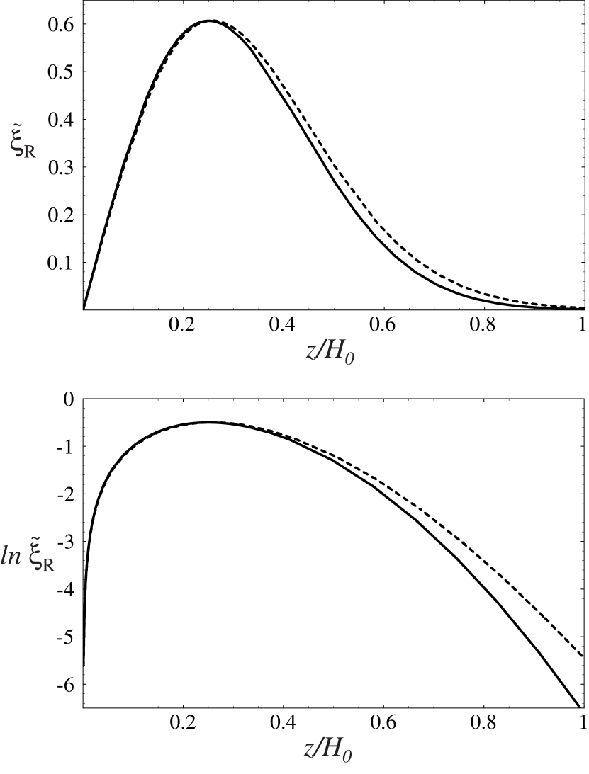
Figure 1: Corrections to the marginally stable solution. The solid line is the analytic marginally-stable solution for the approximation (11) of the density profile, giving $\Lambda=3$. The overlapping dotted line is a numerical solution for the mode in the case of the density distribution $\rho=\rho_{\scriptscriptstyle 0}\exp(-z^{2}/H_{\scriptscriptstyle 0}^{2})$ that gives $\Lambda\simeq 2.9$. Here $\sqrt{k_{\scriptscriptstyle 0}H_{\scriptscriptstyle 0}}=4$, a relatively low value, is chosen to emphasize the difference between the two solutions.

and we see that $k_{\scriptscriptstyle R}$ cannot be too small relative to $k_{\scriptscriptstyle 0}$ in order to have the needed turning points within the main body of the disk. Moreover, if the solution is to be well-localized within the disk the condition $(k_{\scriptscriptstyle 0}H_{\scriptscriptstyle 0})^{2}\gg 1$ corresponding to $\beta_{s}\gg 1$ is necessary. An example of this is illustrated in Fig. 1 where $k_{\scriptscriptstyle 0}H_{\scriptscriptstyle 0}=16$. To illustrate this it may be useful to rewrite Eq. (18) as

$$\left[\exp(-\bar{\bar{\mbox{$z$}}}^{2})-\frac{k_{\scriptscriptstyle R}^{2}}{k_{\scriptscriptstyle 0}^{2}}\right]\tilde{\xi}_{\scriptscriptstyle R}(\bar{\bar{\mbox{$z$}}})+\frac{1}{(k_{\scriptscriptstyle 0}H_{\scriptscriptstyle 0})^{2}}\frac{d^{2}}{d\bar{\bar{\mbox{$z$}}}^{2}}\tilde{\xi}_{\scriptscriptstyle R}(\bar{\bar{\mbox{$z$}}})=0\;,$$

where $\bar{\bar{\mbox{$z$}}}\equiv z/H_{\scriptscriptstyle 0}$. The solution given in Fig. 1 has been obtained numerically and compared to the one that would be found analytically replacing $\exp(-\bar{\bar{\mbox{$z$}}}^{2})$ by $1-\bar{\bar{\mbox{$z$}}}^{2}$ for an equal value of $k_{\scriptscriptstyle 0}H_{\scriptscriptstyle 0}$.

Next we consider the case of unstable ($\gamma_{\scriptscriptstyle 0}\neq 0$) modes that can be found for $\Lambda>3$. We note that the relevant solutions of Eq. (17) are subject to the conditions that in addition to $\tilde{\xi}_{z}$ and $\tilde{\xi}_{\scriptscriptstyle R}$ vanish at large $\bar{z}$. Therefore it is convenient to recast the equation in terms of the variable $\tilde{Y}\propto\rm$, considering that $\tilde{Y}^{\prime}\propto\tilde{\xi}_{z}$ and $\tilde{Y}^{\prime\prime}\propto\tilde{\xi}_{\scriptscriptstyle R}$ given Eqs. (13) and (15). Then we rewrite Eq. (17) as a set of two second-order differential equations

$$\frac{d^{2}}{d\bar{z}^{2}}\tilde{Y}=\bar{\gamma}_{\scriptscriptstyle 0}\tilde{\xi}_{\scriptscriptstyle R}$$ (19)

$$-\frac{d^{2}}{d\bar{z}^{2}}\tilde{\xi}_{\scriptscriptstyle R}+\left(\bar{z}^{2}-\Lambda\right)\tilde{\xi}_{\scriptscriptstyle R}=\bar{\gamma}_{\scriptscriptstyle 0}\tilde{Y}$$ (20)

and note that this set of equations corresponds to the following matricial equation

$$\left(\begin{array}[]{cc}O_{11}&0\\ 0&O_{22}\end{array}\right)\left(\begin{array}[]{c}\tilde{\xi}_{\scriptscriptstyle R}\\ \tilde{Y}\end{array}\right)=\left(\begin{array}[]{cc}\Lambda&\bar{\gamma}_{\scriptscriptstyle 0}\\ \bar{\gamma}_{\scriptscriptstyle 0}&0\end{array}\right)\left(\begin{array}[]{c}\tilde{\xi}_{\scriptscriptstyle R}\\ \tilde{Y}\end{array}\right)$$

where the operators $O_{11}$ and $O_{22}$ are easily identifiable from Eqs. (19) and (20). This has a discrete spectrum of the eigenvalue matrix, when the conditions that both $\tilde{\xi}_{\scriptscriptstyle R}$ and $\tilde{Y}$ are of a given parity and that $\tilde{\xi}_{\scriptscriptstyle R}(\bar{z}^{2}\rightarrow\infty)\rightarrow 0$ and $\tilde{Y}(\bar{z}^{2}\rightarrow\infty)\rightarrow 0$.

Then we refer to the equation for $\tilde{Y}$

$$\frac{d^{4}}{d\bar{z}^{4}}\tilde{Y}-\left(\bar{z}^{2}-\Lambda\right)\frac{d^{2}}{d\bar{z}^{2}}\tilde{Y}+\bar{\gamma}_{\scriptscriptstyle 0}^{2}\tilde{Y}=0$$ (21)

that lends itself to derive the following quadratic form for $\tilde{\xi}_{z}$

$$\left<\left|\tilde{\xi}_{z}^{\prime\prime}\right|^{2}+\bar{z}^{2}\left|\tilde{\xi}_{z}^{\prime}\right|^{2}\right>=\Lambda\left<\left|\tilde{\xi}_{z}^{\prime}\right|^{2}\right>+\bar{\gamma}_{\scriptscriptstyle 0}^{2}\left<\left|\tilde{\xi}_{z}\right|^{2}\right>\;.$$ (22)

This is obtained multiplying Eq. (21) by $d^{2}\tilde{Y}/d\bar{z}^{2}$ and integrating over $\left<-\infty,+\infty\right>$.

The localized solutions for $\bar{z}$ large are given, as in the case where $\bar{\gamma}_{\scriptscriptstyle 0}\rightarrow 0$, by

$$\frac{d^{4}}{d\bar{z}^{4}}\tilde{Y}-\bar{z}^{2}\frac{d^{2}}{d\bar{z}^{2}}\tilde{Y}\simeq 0\;.$$

Thus we have six constraints for the solution of Eq. (21): normalization, two parity conditions, and three unwanted asymptotic limits, for large $\bar{z}$, out of the expected four. Six constraints lead to two eigenvalue conditions: only specific values for both $\Lambda$ and $\bar{\gamma}_{0}$ are allowed, as anticipated on the basis of Eq. (22).

The exact solutions that we have identified for Eq. (21) confirm the general conditions and characteristics that we have outlined. In particular the lowest eigensolution is

$$\tilde{Y}=\exp\left(-\frac{\bar{z}^{2}}{2}\right)\propto\rm$$ (23)

and corresponds to

$$\tilde{\xi}_{z}=\tilde{\xi}_{z,{\scriptscriptstyle 0}}\bar{z}\exp\left(-\frac{\bar{z}^{2}}{2}\right)\propto\frac{d\tilde{Y}}{d\bar{z}}\;,$$

and

$$\tilde{\xi}_{\scriptscriptstyle R}=\tilde{\xi}_{{\scriptscriptstyle R},{\scriptscriptstyle 0}}\left(1-\bar{z}^{2}\right)\exp\left(-\frac{\bar{z}^{2}}{2}\right)\;,$$

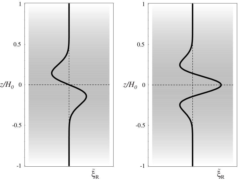
Figure 2: Vertical profiles of the marginally-stable mode (left) and of the lowest unstable mode (right) for $\sqrt{k_{\scriptscriptstyle 0}H_{\scriptscriptstyle 0}}=7$. Here $k_{\scriptscriptstyle 0}=\sqrt{3}\Omega/v_{{\scriptscriptstyle A}z}$, and $H_{\scriptscriptstyle 0}$ is the characteristic scale distance for the density vertical profile near $z=0$. In the figure $z$ is scaled to $H_{\scriptscriptstyle 0}$. The equilibrium density profile is shown as a grayscale background. The value of $k_{\scriptscriptstyle 0}H_{\scriptscriptstyle 0}$ should be sufficiently large that the mode is well-localized over $0\leq|z|\leq H_{\scriptscriptstyle 0}$, e.g. $\tilde{\xi}(z=H_{\scriptscriptstyle 0})/\tilde{\xi}(z=0)\ll 0.1$. Note that the mode is localized over the width $\Delta_{z}\sim H_{\scriptscriptstyle 0}/\sqrt{k_{\scriptscriptstyle 0}H_{\scriptscriptstyle 0}}$ and that $(k_{\scriptscriptstyle 0}H_{\scriptscriptstyle 0})^{1/2}\sim\beta_{s}^{1/4}$. Therefore the corresponding values of $\beta_{s}$ are very large.

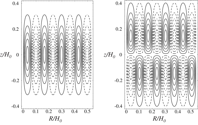
Figure 3: Two-dimensional streamline patterns of the plasma displacement for the marginally-stable mode (left) and the lowest unstable mode (right). Solid versus dotted lines denote the sign of rotation. Length units in the figure are scaled to $H_{\scriptscriptstyle 0}$. As noted in the text, the radial variation of the mode is faster than its vertical variation, which is in turn stronger than the vertical variation of the density profile. Here $\sqrt{k_{\scriptscriptstyle 0}H_{\scriptscriptstyle 0}}=7$.

as shown in Figs. 2 and 3. We note that, for $\tilde{Y}(\bar{z})$ given by Eq. (23), $\tilde{Y}^{\prime\prime\prime\prime}=(\bar{z}^{2}-1)\tilde{Y}^{\prime\prime}+2\tilde{Y}+4\bar{z}\tilde{Y}^{\prime}$ and find $\Lambda=5$, $\bar{\gamma}_{\scriptscriptstyle 0}^{2}=2$ from the condition $3-\bar{\gamma}_{0}^{2}-\Lambda-(5-\Lambda)\bar{z}^{2}=0$. Thus the relevant growth rate is

$$\gamma_{\scriptscriptstyle 0}=\left(\frac{6}{7}\right)^{1/2}\frac{v_{{\scriptscriptstyle A}z}}{H_{\scriptscriptstyle 0}}\ll\Omega$$ (24)

and

$$\delta k_{\scriptscriptstyle R}=-\frac{5}{2H_{\scriptscriptstyle 0}}$$ (25)

The next eigenfunction $\tilde{Y}=\bar{z}\exp(-\bar{z}^{2}/2)$ corresponds to $\tilde{\xi}_{z}=\tilde{\xi}_{z,{\scriptscriptstyle 0}}(1-\bar{z}^{2})\exp(-\bar{z}^{2}/2)$ and $\tilde{\xi}_{\scriptscriptstyle R}=\tilde{\xi}_{{\scriptscriptstyle R},{\scriptscriptstyle 0}}\bar{z}(3-\bar{z}^{2})\exp(-\bar{z}^{2}/2)$. The relevant set of eigenvalues is $\Lambda=7$, $\bar{\gamma}_{\scriptscriptstyle 0}^{2}=6$. Moreover, there are two even-parity solutions at $\Lambda=9$, two odd solutions at $\Lambda=11$, three at 13 and 15, and so on up to higher and higher eigenvalues, as indicated in Table 1.

We observe that the eigenfunctions with the highest values of $\bar{\gamma}_{\scriptscriptstyle 0}^{2}$ corresponding to the same value of $\Lambda$ (that is, the most unstable solutions) are, in fact, given by

$$\tilde{Y}(\bar{z})=H_{n}\left(\frac{\bar{z}}{\sqrt{2}}\right)e^{-\bar{z}^{2}/2}$$ (26)

$$\Lambda=5+2n$$ (27)

$$\bar{\gamma}_{\scriptscriptstyle 0}^{2}=(n+1)(n+2)\;.$$ (28)

The problem can be dealt with more simply by noting that the Fourier transform of the relevant solutions satisfy the following second-order equation

$$k_{\bar{z}}^{2}\frac{d^{2}}{dk_{\bar{z}}^{2}}\tilde{Y}(k_{\bar{z}})+4k_{\bar{z}}\frac{d}{dk_{\bar{z}}}\tilde{Y}(k_{\bar{z}})+(\Lambda k_{\bar{z}}^{2}-\bar{\gamma}_{0}^{2}+2-k_{\bar{z}}^{4})\,\tilde{Y}=0$$

whose solutions corresponding to Eq. (26) are

$$\tilde{Y}(k_{\bar{z}})=k_{\bar{z}}^{n}\exp\left(-\frac{k_{\bar{z}}^{2}}{2}\right)$$

For these solutions we have

$$2+3n+n^{2}-\bar{\gamma}_{0}^{2}+(\Lambda-5-2n)\,k_{\bar{z}}^{2}=0$$

which gives the conditions (27) and (28). Combining the two, we obtain the dispersion relation

$$\bar{\gamma}_{\scriptscriptstyle 0}^{2}=\frac{1}{4}(\Lambda-3)(\Lambda-1)$$ (29)

where $\Lambda\geq 3$ takes integer odd values.

5 Quasi-localized Modes

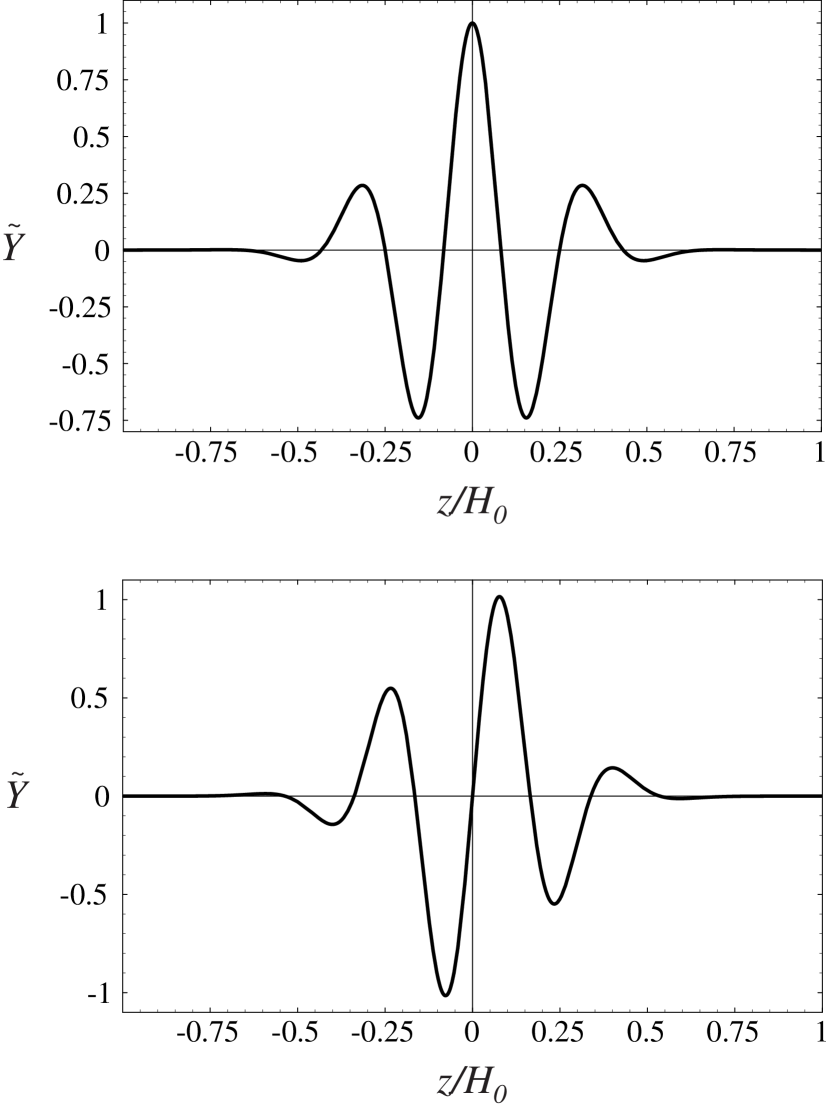
Figure 4: Profiles of a localized even mode (upper) and of an odd quasi-localized mode (lower) for $\Lambda=13$ and $\gamma_{\scriptscriptstyle 0}^{2}=30$. The decay of the even mode is proportional to a Gaussian while that of the odd mode is proportional to $\bar{\bar{\mbox{$z$}}}^{-5}$, where $\bar{\bar{\mbox{$z$}}}\equiv z/H$. Here $\sqrt{k_{\scriptscriptstyle 0}H_{\scriptscriptstyle 0}}=7$.

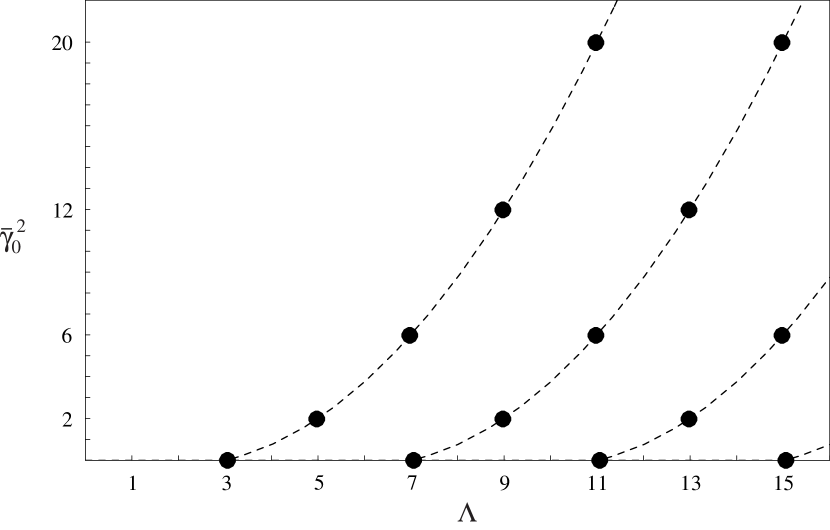
Figure 5: Graphic representation of the dispersion relation for the axisymmetric ballooning modes. The marginally-stable modes ($\bar{\gamma}_{\scriptscriptstyle 0}=0$) and the unstable modes ($\bar{\gamma}_{\scriptscriptstyle 0}>0$) corresponding to discrete and odd values of $\Lambda$ are indicated by dots. Additional branches of solutions with similar behavior exist at multiples of 4 at higher $\Lambda$. Clearly the highest branch corresponding to the highest growth rates for a given value of $\Lambda$ is the meaningful one. The continuous spectrum of quasi-localized modes is indicated by a dotted line, but in practice they cannot be considered as physically acceptable unless $\bar{\gamma}_{\scriptscriptstyle 0}^{2}\geq 30$, a value that exceeds the asymptotic conditions under which the mode equation (21) has been derived.

In addition to the well-localized modes with the discrete spectrum discussed in the previous section, there is a class of modes to consider which decay algebraically rather than exponentially as a function of $\bar{z}$ and that have a continuous spectrum (see Figs. 4 and 5). Therefore we may classify them as quasi-localized modes and, in practice, consider only those which have relatively fast power-law decays such as $\tilde{Y}\sim 1/{\bar{z}}^{\alpha}$ with $\alpha>5$ as physically relevant.

The asymptotic solutions for $|\bar{z}|\rightarrow\infty$ of the mode equation that depend algebraically on $\bar{z}$ are given by

$$\frac{d^{2}}{d\bar{z}^{2}}\tilde{Y}-\bar{\gamma}_{0}^{2}\tilde{Y}\simeq 0\;,$$

and are of the form

$$\tilde{Y}\propto\bar{z}^{1/2\pm\sqrt{1/4+\bar{\gamma}_{0}^{2}}}$$ (30)

The “practical” condition $\alpha>5$ corresponds to $\bar{\gamma}_{\scriptscriptstyle 0}^{2}>30$ which can be considered to exceed the asymptotic limit (12) for which the mode equation (21) has been derived, unless $k_{\scriptscriptstyle 0}^{2}H_{\scriptscriptstyle 0}^{2}$ has extremely large values such that $30<\bar{\gamma}_{\scriptscriptstyle 0}^{2}\ll k_{\scriptscriptstyle 0}H_{\scriptscriptstyle 0}$.

The four asymptotic solutions of the fourth-order equation are: decaying exponential, decaying power-law, growing exponential, and growing power-law. The last two are of course unacceptable. Excluding only the growing solutions, we are left with five conditions on a fourth-order equation. This leads to one eigenvalue condition, corresponding to $\bar{\gamma}_{0}$ being a continuous function of $\Lambda$.

Since the discrete solutions are a special case of the continuous spectrum formed by a linear combination of Gaussian-decaying and power-law decaying asymptotic forms, we consider that Eq. (29) remains valid for continuously varying values of $\Lambda$. Then we note that $\bar{\gamma}_{\scriptscriptstyle 0}^{2}>30$ corresponds to $\Lambda>13$.

We may observe that when $\Lambda$ and $\bar{\gamma}_{\scriptscriptstyle 0}^{2}$ are related by Eq. (29), Eq. (21) can be factored as follows:

$$\left(\frac{d^{2}}{d\bar{z}^{2}}-\bar{z}\frac{d}{d\bar{z}}+\frac{\Lambda-1}{2}\right)\left(\frac{d^{2}}{d\bar{z}^{2}}\tilde{Y}+\bar{z}\frac{d}{d\bar{z}}\tilde{Y}+\frac{\Lambda-3}{2}\tilde{Y}\right)=0$$ (31)

This factorization separates the growing from the decaying asymptotic solutions. Thus

$$\tilde{Y}\simeq c_{\scriptscriptstyle 1}\exp\left(-\frac{\bar{z}^{2}}{2}\right)+c_{\scriptscriptstyle 2}\frac{1}{\bar{z}^{(\Lambda-3)/2}}$$

The discrete spectrum corresponds to values of $\Lambda$ for which $c_{\scriptscriptstyle 2}=0$. A relevant case is illustrated in Fig. 4.

We note that the second-order equation resulting from Eq. (31) can be solved analytically in general. Introducing the variable $u\equiv-\bar{z}^{2}/2$, we have

$$u\frac{d^{2}}{du^{2}}\tilde{Y}(u)+\left(\frac{1}{2}-u\right)\frac{d}{du}\tilde{Y}(u)-\left(\frac{\Lambda-3}{4}\right)\tilde{Y}(u)=0$$

which is the standard differential equation for the confluent hypergeometric function ${}_{1}F_{1}$, also known as the Kummer function:

$$\tilde{Y}_{\mathrm{even}}(\bar{z})={}_{1}F_{1}\left(\frac{\Lambda-3}{4},\frac{1}{2},-\frac{\bar{z}^{2}}{2}\right)$$

$$\tilde{Y}_{\mathrm{odd}}(\bar{z})=\bar{z}\;{}_{1}F_{1}\left(\frac{\Lambda-1}{4},\frac{3}{2},-\frac{\bar{z}^{2}}{2}\right)$$

For discrete choices of $\Lambda$ and particular parities, these Kummer functions simplify to the localized solutions of Eq. (26), but in general they have power-law decays at large $\bar{z}$, and solutions exist of either parity at the same eigenvalues.

6 Observations

For the modes that have been presented, it is clear that $\Lambda$ will have to be limited by the condition that $\gamma_{\scriptscriptstyle 0}^{2}\sim v_{{\scriptscriptstyle A}z}^{2}/H_{\scriptscriptstyle 0}^{2}\ll\Omega^{2}$. Therefore unless $v_{{\scriptscriptstyle A}z}^{2}/c_{s}^{2}$ is exceedingly small very few modes can be fitted in the interval $5\leq\Lambda\ll k_{\scriptscriptstyle 0}H_{\scriptscriptstyle 0}\sim\beta_{s}^{1/2}$. Thus a problem which arises is that of identifying a physical factor which can localize radially the normal modes considered; a mode packet, constructed by varying $\Lambda$ over a significant interval, is difficult to envision.

We note also that, by comparison with the “long cylinder” modes, the “cost” of localizing a mode vertically between $z=-H$ and $z=+H$ and creating the needed turning points in the appropriate equation involves (i) the requirement that $k_{\scriptscriptstyle R}$ be significant and related to the scale of vertical localization $\Delta_{z}\sim(H_{\scriptscriptstyle 0}/k_{\scriptscriptstyle 0})^{1/2}$ with $k_{\scriptscriptstyle R}\Delta_{z}\gg 1$ and $k_{\scriptscriptstyle R}\simeq k_{\scriptscriptstyle 0}$ ; (ii) a considerable reduction of the growth rate $\gamma_{\scriptscriptstyle 0}$ relative to $\Omega$ and its dependence on the scale distance $H_{\scriptscriptstyle 0}$. If a physical factor providing the radial localization of the discrete modes given by Eq. (21) can be found it is reasonable to expect that the resulting growth rate will depend on a second scale distance and that it should be depressed further relative to the expression (24). In order to resolve the issue of the radial localization of the mode, the best option may be that of attempting to superpose modes centered around a range of values of $R_{\scriptscriptstyle 0}$, taking into account that the corresponding values of $k_{\scriptscriptstyle R}$, $\gamma_{\scriptscriptstyle 0}$, and $\Delta_{z}$ vary as a function of $R_{\scriptscriptstyle 0}$.

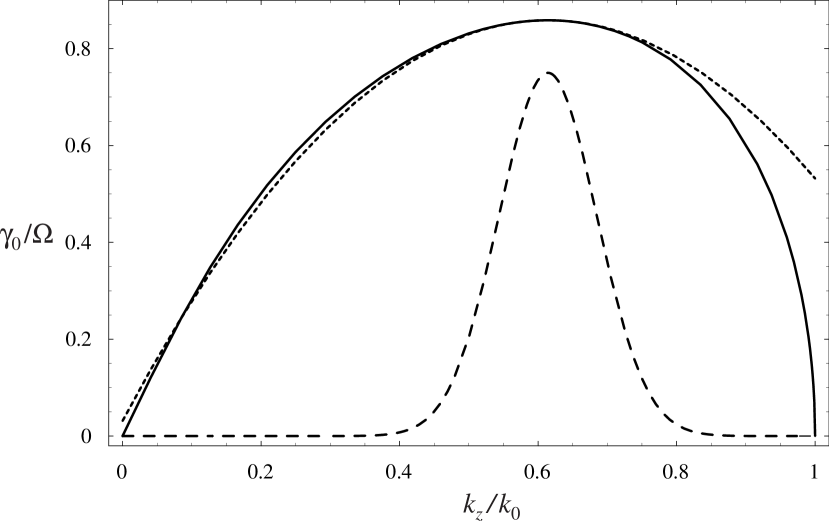
Figure 6: Dispersion relation of the MRI modes. This plot shows the growth rate of the MRI modes as a function of $k_{z}$ when $k_{\scriptscriptstyle R}=0$. The maximum growth rate of $\gamma_{\scriptscriptstyle 0}\simeq 0.85\Omega$ occurs at $k_{z}\simeq 0.6k_{\scriptscriptstyle 0}$, and the region of instability is bounded by $k_{\scriptscriptstyle R}^{2}+k_{z}^{2}<k_{\scriptscriptstyle 0}^{2}$. Here $k_{\scriptscriptstyle 0}=\sqrt{3}\Omega/v_{{\scriptscriptstyle A}z}$. The short dashed line gives the approximation (32) to the dispersion relation. The long dashed line is a sample wavepacket with $\Delta=10k_{\scriptscriptstyle 0}^{-1}$ centered around the peak growth rate, shown for comparison with the accuracy of the approximation. Clearly, narrower spectra for $k_{z}$ could be chosen, but they would correspond to larger values of $\Delta$.

The argument could be made that by taking very small wavelengths, requiring that very large values of $\beta_{s}$ be considered, the MRI dispersion relation (10) could be used with $k_{\scriptscriptstyle R}^{2}\ll k_{z}^{2}$ (see Fig. 6). Then “large” growth rates would be obtained, but wave packets would have to be constructed to ensure that the resulting non-normal mode would be localized vertically. However, we can argue easily that a packet can spread rapidly, losing its initial localization property. In particular we consider an interval of values of $k_{z}$ around $k_{z}=k_{z}^{\scriptscriptstyle 0}$ where the growth rate given by Eq. (10) is maximum. Therefore in this interval,

$$\gamma_{\scriptscriptstyle 0}(k_{z})\simeq\gamma_{\scriptscriptstyle 0}(k_{z}^{\scriptscriptstyle 0})+\frac{1}{2}\frac{\partial^{2}\gamma_{\scriptscriptstyle 0}}{\partial k_{z}^{2}}(k_{z}-k_{z}^{\scriptscriptstyle 0})^{2}\;,$$ (32)

where $\partial^{2}\gamma_{\scriptscriptstyle 0}/\partial k_{z}^{2}<0$, and $\partial\gamma_{\scriptscriptstyle 0}/\partial k_{z}=0$ for $k_{z}=k_{z}^{\scriptscriptstyle 0}$. Then we construct the packet

$$\Psi \propto \left[\int dk_{z}\exp\left\{-\Delta^{2}(k_{z}-k_{z}^{\scriptscriptstyle 0})^{2}+\frac{1}{2}\frac{\partial^{2}\gamma_{\scriptscriptstyle 0}}{\partial k_{z}^{2}}t(k_{z}-k_{z}^{\scriptscriptstyle 0})^{2}+i(k_{z}-k_{z}^{\scriptscriptstyle 0})z\right\}\right]$$

$$\exp\Big{[}\gamma_{\scriptscriptstyle 0}(k_{z}^{\scriptscriptstyle 0})t+ik_{z}^{\scriptscriptstyle 0}z+ik_{\scriptscriptstyle R}(R-R_{\scriptscriptstyle 0})\Big{]}$$

and we obtain

$$\Psi\propto\exp\left\{-\frac{z^{2}}{4\left[\Delta^{2}-\frac{1}{2}\frac{\partial^{2}\gamma_{\scriptscriptstyle 0}}{\partial k_{z}^{2}}t\right]}+\gamma_{\scriptscriptstyle 0}t+ik_{z}^{\scriptscriptstyle 0}z\right\}$$ (34)

where $\Delta^{2}\ll H^{2}$. It is evident that the packet begins to spread for ${k_{z}^{\scriptscriptstyle 0}}^{2}(\partial^{2}\gamma_{\scriptscriptstyle 0}/\partial k_{z}^{2})t\sim 2\Delta^{2}{k_{z}^{\scriptscriptstyle 0}}^{2}$.

In order to estimate the rate of angular momentum transport that these packets may produce we derive the flux of angular momentum from the quasilinear theory of the unconfined normal modes that are the mode packet components. Clearly,

$$\Gamma_{J}=R\left[\rho v_{\scriptscriptstyle\phi}v_{\scriptscriptstyle R}-\frac{1}{4\pi}B_{\scriptscriptstyle\phi}B_{\scriptscriptstyle R}\right]\;.$$

Considering the perturbations from the equilibrium state, the flux $\Gamma_{J}$ can be separated into an average and a fluctuating part: $\Gamma_{J}=\left<\Gamma_{J}\right>+\hat{\Gamma}_{J}$ where $\big{<}\tilde{\Gamma}_{J}\big{>}=0$. In particular $\big{<}\Gamma_{J}\big{>}=\sum_{k}\big{<}\Gamma_{Jk}\big{>}$ and we note that the particle flux associated with these modes $\big{<}\Gamma_{p}\big{>}$ is null as $\big{<}\hat{\rho}\hat{v}_{\scriptscriptstyle R}\big{>}=0$ given the fact that $\nabla\cdot\mathbf{\hat{v}}=0$ and $\hat{\rho}=0$. Then

$$\left<\Gamma_{Jk}\right>=\rho\left<\hat{v}_{{\scriptscriptstyle\phi}k}\hat{v}_{{\scriptscriptstyle R}k}^{*}\right>-\frac{1}{4}\left<\hat{B}_{{\scriptscriptstyle\phi}k}\hat{B}_{{\scriptscriptstyle R}k}^{*}\right>+\mathrm{c.c.}$$ (35)

where $\hat{v}_{{\scriptscriptstyle R}k}=\gamma_{{\scriptscriptstyle 0}k}\hat{\xi}_{{\scriptscriptstyle R}k}$, $\hat{v}_{{\scriptscriptstyle\phi}k}=-\Omega^{\prime}R\hat{\xi}_{{\scriptscriptstyle R}k}+\gamma_{{\scriptscriptstyle 0}k}\hat{\xi}_{{\scriptscriptstyle\phi}k}$, $\hat{B}_{{\scriptscriptstyle R}k}=i(k_{z}B_{z})\hat{\xi}_{{\scriptscriptstyle R}k}$, and $\hat{B}_{{\scriptscriptstyle\phi}k}=i(k_{z}B_{z})\hat{\xi}_{{\scriptscriptstyle\phi}k}$. For $G_{k}\equiv\big{<}\Gamma_{Jk}/(\rho R)\big{>}$ we obtain

$$G_{k}=2\gamma_{{\scriptscriptstyle 0}k}\left<\left|\hat{\xi}_{{\scriptscriptstyle R}k}\right|^{2}\right>\left[-\Omega^{\prime}R+2\Omega\frac{\omega_{{\scriptscriptstyle A}z}^{2}-\gamma_{{\scriptscriptstyle 0}k}^{2}}{\omega_{{\scriptscriptstyle A}z}^{2}+\gamma_{{\scriptscriptstyle 0}k}^{2}}\right]$$ (36)

and the relevant effective diffusion coefficient can be defined as

$$\mathcal{D}_{\mathrm{eff}}\simeq 2\gamma_{{\scriptscriptstyle 0}k}\left<\left|\hat{\xi}_{{\scriptscriptstyle R}k}\right|^{2}\right>\left[1-\frac{2\Omega}{\Omega^{\prime}R}\,\frac{\omega_{{\scriptscriptstyle A}z}^{2}-\gamma_{{\scriptscriptstyle 0}k}^{2}}{\omega_{{\scriptscriptstyle A}z}^{2}+\gamma_{{\scriptscriptstyle 0}k}^{2}}\right]\;.$$ (37)

We note that the transport of angular momentum, produced by modes of the considered type for which $\nabla\cdot\hat{\mathbf{v}}=0$ and evaluated from the relevant quasilinear theory assuming the adiabatic equation of state, is not accompanied by an increase of thermal energy. This is an important feature that differentiates the effects of these modes from those of a viscous diffusion coefficient.

Using the dispersion relation (10) we can verify that $\mathcal{D}_{\mathrm{eff}}$ is positive. To assess the order of magnitude of $\mathcal{D}_{\mathrm{eff}}$ we may argue, as is usually done in plasma physics, that, at saturation, $|\tilde{\xi}_{\scriptscriptstyle R}|\sim 1/k_{z}^{\scriptscriptstyle 0}\sim 1/k_{\scriptscriptstyle 0}$. Thus we have

$$\mathcal{D}_{\mathrm{eff}}\sim\frac{\gamma_{\scriptscriptstyle 0}}{k_{\scriptscriptstyle 0}^{2}}\sim\left(\frac{\gamma_{\scriptscriptstyle 0}}{\Omega}\right)\frac{v_{\scriptscriptstyle A}^{2}}{\Omega}\sim\left(\frac{\gamma_{\scriptscriptstyle 0}}{\Omega}\right)c_{s}\frac{H}{\beta_{s}}\;.$$ (38)

Since the existence of these modes requires that $\beta_{s}\gg 1$ we may conclude that this kind of mode packet should not produce a rate of transport of angular momentum that is comparable with the one represented by the Shakura-Sunyaev coefficient (Shakura & Sunyaev, 1973)

$$\mathcal{D}_{ss}\simeq\alpha_{ss}c_{s}H\;.$$ (39)

This is frequently used with ad hoc values of the numerical coefficient $\alpha_{ss}$ that exceed $10^{-2}$.

It is evident that the mode packets have the intrinsic limitations of not being the normal modes of the system when considering their possible excitation. In particular we may consider their growth to be limited to the case where

$$\Delta^{2}-\frac{1}{2}\frac{\partial^{2}\gamma_{\scriptscriptstyle 0}}{\partial k_{z}^{2}}t<\frac{H_{\scriptscriptstyle 0}^{2}}{\alpha_{{\scriptscriptstyle H}}^{2}}$$

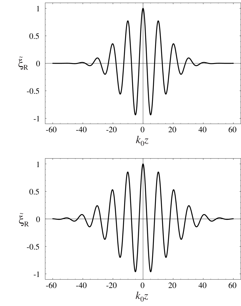
Figure 7: Spreading of non-normal mode packets. An initially contained mode packet formed from a range of $k_{z}$ centered around the peak growth rate of the MRI will spread over time due to the dispersion relation. The top panel gives an initial packet with a width $\Delta=10k_{\scriptscriptstyle 0}^{-1}$ at $t=0$, and the bottom panel shows the same packet at $\gamma_{\scriptscriptstyle 0}t=25$. Here $k_{\scriptscriptstyle 0}=\sqrt{3}\Omega/v_{{\scriptscriptstyle A}z}$, and the width $\Delta$ is chosen by the criterion that the mode packet undergoes minimal deformation as a function of time while having the maximum growth rate. The length is given in units of $k_{\scriptscriptstyle 0}^{-1}$, so one can see that the mode packet is unacceptably spread even at $t=0$ for $k_{\scriptscriptstyle 0}H_{\scriptscriptstyle 0}<30$ (corresponding to $\beta_{s}\sim 1000$), and even higher values of $\beta_{s}$ are necessary to retain containment through many orbit times.

where $\alpha_{{\scriptscriptstyle H}}$ is a reasonable numerical coefficient such as 3. A numerical derivation of the mode packet (34) deriving $\partial^{2}\gamma_{\scriptscriptstyle 0}/\partial k_{z}^{2}$ from the dispersion relation (10) is given in Fig. 7. We note that the packet spreads rather slowly as a function of time, as $\Delta_{\mathrm{eff}}=[\Delta^{2}-(\partial^{2}\gamma_{\scriptscriptstyle 0}/\partial k_{z}^{2})t]^{1/2}$. On the other hand the initial spread $\Delta$ has to be relatively broad as the dispersion relation (10) limits the range of values of $k_{z}$ for which Eq. (32) is valid, as indicated in Fig. 6. The consequence of this is that the packet spread can reach the region where the Alfvén velocity varies significantly relative to its central value even at the outset.

When dealing with normal modes that are contained within the disk, given the discrete spectrum of both $k_{\scriptscriptstyle R}$ and $\gamma_{\scriptscriptstyle 0}$ that characterize them and that the vertical eigenfunctions are of the ballooning type, the standard quasilinear theory cannot be applied to arrive at an estimate of $\mathcal{D}_{\mathrm{eff}}$. We may in fact use the expression (38) which can be arrived at by standard qualitative considerations, and conclude that the relevant values of $\mathcal{D}_{\mathrm{eff}}$ would fall well below those estimated from Eq. (39). On the other hand, the greatest difficulty that the ballooning modes have is that on envisioning a process by which they can be localized radially.

Appendix A Higher Branch Solutions

We note that additional branches of solutions to Eq. (21) also exist at higher $\Lambda$ at exact intervals of 4, but with lower corresponding values of $\bar{\gamma}_{\scriptscriptstyle 0}^{2}$. For completeness, the solutions for branch $m\geq 0$ are given by:

$$\tilde{Y}_{\mathrm{even}}(\bar{z})=\sum_{i=0}^{m}a_{m,i}(\Lambda)\;{}_{1}F_{1}\left(i-m+\frac{\Lambda-3}{4},\frac{1}{2},-\frac{\bar{z}^{2}}{2}\right)$$

$$\tilde{Y}_{\mathrm{odd}}(\bar{z})=\bar{z}\;\sum_{i=0}^{m}b_{m,i}(\Lambda)\;{}_{1}F_{1}\left(i-m+\frac{\Lambda-1}{4},\frac{3}{2},-\frac{\bar{z}^{2}}{2}\right)$$

where the coefficient functions are given recursively by:

$$a_{m,i}(\Lambda)=\frac{(i-m-1)(\Lambda+4i-4m-7)}{i(\Lambda+2i-4m-2)}\;a_{m,i-1}(\Lambda)$$

$$b_{m,i}(\Lambda)=\frac{(i-m-1)(\Lambda+4i-4m-5)}{i(\Lambda+2i-4m-2)}\;b_{m,i-1}(\Lambda)$$

with the base case given by normalization: $a_{m,0}(\Lambda)=b_{m,0}(\Lambda)=1$. The dispersion relation for the higher branches is

$$\bar{\gamma}_{\scriptscriptstyle 0}^{2}=\frac{(\Lambda-4m-3)(\Lambda-4m-1)}{4}$$

with $\Lambda>3+4m$.

Table 1: Normal Mode Solutions

$\Lambda$	$\bar{\gamma}_{\scriptscriptstyle 0}^{2}$	$\tilde{Y}(\bar{z})$
5	2	$e^{-\bar{z}^{2}/2}$
7	6	$\bar{z}\,e^{-\bar{z}^{2}/2}$
9	12	$(1-\bar{z}^{2})\,e^{-\bar{z}^{2}/2}$
9	2	$(1+\frac{2}{3}\bar{z}^{2})\,e^{-\bar{z}^{2}/2}$
11	20	$(\bar{z}-\frac{1}{3}\bar{z}^{3})\,e^{-\bar{z}^{2}/2}$
11	6	$(\bar{z}+2\bar{z}^{3})\,e^{-\bar{z}^{2}/2}$
13	30	$(1-2\bar{z}^{2}+\frac{1}{3}\bar{z}^{4})\,e^{-\bar{z}^{2}/2}$
13	12	$(1+\bar{z}^{2}-\frac{2}{3}\bar{z}^{4})\,e^{-\bar{z}^{2}/2}$
13	2	$(1+\frac{4}{19}\bar{z}^{2}+\frac{4}{19}\bar{z}^{4})\,e^{-\bar{z}^{2}/2}$