Inter-Network magnetic fields
observed with sub-arcsec resolution

We analyze a time sequence of Inter-Network (IN) magnetograms observed at the solar disk center. Speckle reconstruction techniques provide a good spatial resolution (0$\aas@@fstack{\prime\prime}$5 cutoff frequency) yet maintaining a fair sensitivity (some 20 G). Patches with signal above noise cover 60 % of the observed area, most of which corresponds to intergranular lanes. The large surface covered by signal renders a mean unsigned magnetic flux density between 17 G and 21 G (1 G$\equiv$ 1 Mx cm^-2). The difference depends on the spectral line used to generate the magnetograms (Fe i $\lambda$6302.5 Å or Fe i $\lambda$6301.5 Å). Such systematic difference can be understood if the magnetic structures producing the polarization have intrinsic field strengths exceeding 1 kG, and consequently, occupying only a very small fraction of the surface (some 2%). We observe both, magnetic signals changing in time scales smaller than 1 min, and a persistent pattern lasting longer than the duration of the sequence (17 min). The pattern resembles a network with a spatial scale between 5 and 10 arcsec, which we identify as the mesogranulation. The strong dependence of the polarization signals on spatial resolution and sensitivity suggests that much quiet Sun magnetic flux still remains undetected.

1 Introduction

Most of the solar surface appears as non-magnetic in traditional magnetic field determinations (e.g., in the full-disk Kitt Peak magnetograms; Jones et al. 1992). This so-called quiet Sun does not produce enough polarization to show up in the measurements. However, such lack of detection does not imply the non-existence or irrelevance of the quiet Sun magnetism. On the contrary, the limited sensitivity of the standard magnetograms and the large area covered by the quiet Sun point out that traditional measurements may easily overlook a large fraction of the solar magnetic flux. With various flavors and shades, this argument has been put forward many times during the past fifty years (e.g. Unno 1959; Stenflo 1982; Zirin 1987; Yi et al. 1993; Sánchez Almeida 1998, 2003). If the conjecture were correct and the quiet Sun carries a sizeable fraction of the existing magnetic flux, then weak polarization signals should appear upon improvement of the sensitivity of the magnetograms. Such weak signals are actually observed thanks to the last generation of solar spectro-polarimeters. When the noise is in the few G level and the angular resolution about 1″, then most of the solar surface becomes magnetic (e.g., Grossmann-Doerth et al. 1996; Lin & Rimmele 1999; Lites 2002). In addition, Hanle depolarization measurements of chromospheric lines also indicate the presence of an ubiquitous magnetic field (e.g., Faurobert-Scholl et al. 1995; Bianda et al. 1999; Shchukina & Trujillo Bueno 2003).

Little is known about the physical properties of these fields (magnetic flux, distribution of field strengths, structure, degree of concentration and tangling, relationship with the fields in the chromosphere and corona, etc.). The observational studies are still exploratory, aiming at setting up the scene. With this general purpose, we have observed the magnetic fields of an Inter-Network (IN) region with good angular resolution, yet maintaining a fair sensitivity. The study refers to low flux features in the interior of a network cell, excluding network patches for which an extensive literature exists (e.g., Solanki 1993; Stenflo 1994). IN magnetic fields were already discovered in the seventies (Livingston & Harvey 1975; Smithson 1975). During the last decade, with the new observational and diagnostic capabilities, these IN fields have received increasing attention. So far only a fraction of the IN field has been detected. This conclusion follows from the presence of unresolved mixed polarities in 1″ angular resolution observations (e.g., Sánchez Almeida et al. 1996; Sánchez Almeida & Lites 2000; Lites 2002). The mixing of polarities reduces the polarization, making the IN magnetic structures difficult to identify. It is therefore to be expected that more locations with magnetic fields will be detected when increasing the spatial resolution. Some of the recent observational studies find IN fields having magnetic field strengths substantially lower than 1 kG (Keller et al. 1994; Lin 1995; Lin & Rimmele 1999; Bianda et al. 1998, 1999; Khomenko et al. 2003). On the contrary, different observing and interpretation techniques indicate the existence of strong kG magnetic fields (Grossmann-Doerth et al. 1996; Sigwarth et al. 1999; Sánchez Almeida & Lites 2000; Socas-Navarro & Sánchez Almeida 2002). The inconsistency could be cured if the IN regions present a continuous distribution of field strengths. Depending on the specificities of the diagnostic technique, one is mostly sensitive to a particular part of such distribution (see Cattaneo 1999; Sánchez Almeida & Lites 2000; Socas-Navarro & Sánchez Almeida 2003). Lifetimes of IN features have been measured to be between 0.2 to 7.5 hours (Zhang et al. 1998). Improving of the angular resolution and cadence reduces the lifetimes, which come down to a few minutes (Lin & Rimmele 1999). Such combination of short lifetimes with the large flux content makes IN regions a very efficient system to process magnetic fields, orders of magnitude more effective than both active regions (uplifting $\leavevmode\nobreak\ 7\,\times\,10^{21}$ Mx day^-1 during the maximum of the cycle, Harvey-Angle 1993) and ephemeral regions ($\sim\,5\,\times\,10^{23}$ Mx day^-1, Hagenaar 2001).

Here we measure several basic physical properties of the IN fields. The novel side of the study lies in the good spatial resolution of the time series of magnetograms on which the measurements are based (0$\aas@@fstack{\prime\prime}$5). The observations are presented in Sect. 2. Then Sect. 3 describes how the high spatial resolution is obtained by speckle reconstruction, and how the magnetograms are produced from the reconstructed spectro-polarimetric maps. We analyze in detail the best snapshot of the sequence to characterize the properties of the IN fields (Sect. 4). The complete series allows us to study the time evolution of the magnetic signals (Sect. 5). In order to assess the reliability of our conclusions, we analyze in detail the consistency of the results, both internally and when compared with previous measurements (Sect. 6). Some of the results presented here were already advanced in a letter by Domínguez Cerdeña et al. (2003).

2 Observations

The observations were obtained with the Göttingen Fabry-Perot Interferometer (FPI), which is a post-focus instrument of the German Vacuum Tower Telescope of the Observatorio del Teide (Tenerife, Spain). The target was a very quiet Sun region near disk center, which was selected using G-band video images to avoid contamination from network magnetic concentrations. The optical system derives from the early work by Bendlin et al. (1992), Bendlin (1993), and Bendlin & Volkmer (1995). Its present setup is described in Koschinsky et al. (2001). It includes two CCD cameras, operating simultaneously, with an exposure time of 30 ms. Both CCDs have 384$\times$286 pixels, each pixel being 0$\aas@@fstack{\prime\prime}$1 $\times$ 0$\aas@@fstack{\prime\prime}$1 on the Sun, which corresponds to half the diffraction limit of the telescope at the working wavelength. The broad-band camera (CCD1) images the field-of-view (FOV) through an interference filter (band-pass $\sim\,$100 Å, centered at $\sim\,$6300 Å). It provides the so-called speckle image, needed for the speckle reconstruction (Sect. 3.1). The second camera (CCD2) gathers narrow-band images whose wavelength is selected by the FPI. This second beam includes a Stokes $V$ analyzer, which separates the left and right circularly polarized components of the light into different areas of the CCD2 (for details, see Fig. 1 in Koschinsky et al. 2001; Koschinsky 2001). The FPI allows to scan in wavelength, taking several images per wavelength position. We select a spectral region around $\lambda$6302 Å, which contains the iron lines Fe i $\lambda$6301.5 Å (Landé factor $g_{L}=1.67$), Fe i $\lambda$6302.5 Å ($g_{L}=2.5$), as well as the telluric line O₂ $\lambda$6302.8 Å. The FPI wavelength step was set to 31.8 mÅ, which suffices to sample the telluric line (5 wavelengths, with 2 images per position), and the two Fe i lines (14 positions each, with 5 images per position). The dots in Fig. 1 indicate the exact wavelengths. A full scan with the properties described above renders 150 images, which is the maximum number allowed by the acquisition system. Each scan lasts 35 s, plus 15 s needed for storage onto hard disk.

The FPI was adjusted to yield a band-pass of 44 mÅ FWHM (Full Width Half Maximum). This finite wavelength resolution modifies the spectrum. Figure 1 shows the mean Stokes $I$ profile in one of our flatfields, together with the spectrum of the disk center as published in a standard solar atlas (Brault & Neckel 1987, quoted in Neckel 1999). Note the good agreement between our spectrum and the atlas smeared with the theoretical band-pass of the FPI.

The data used in the work belong to a short time series of 20 scans taken in April 29, 2002. The cadence was some 50 s, so that the series spans 17 min. The seeing conditions were particularly good, with a Fried parameter deduced from the speckle reconstruction between $13$ and $14$ cm.

Figure 1: Comparison between a Stokes $I$ profile from our flat field data (open circles) and a reference solar spectrum before (dotted line) and after (solid line) convolution with the FPI band-pass function (FWHM 44 mÅ). The wavelength $\lambda$ is referred to 6300 Å, and the Stokes $I$ profiles are normalized to the continuum intensity $I_{c}$.

3 Data analysis

3.1 Speckle reconstruction of the narrow-band images

Figure 2: Filters and power spectra involved in the process of image restoration. a) Solid line: noise filter applied to the series of individual frames that give rise to each restored image. Dashed line: optical transfer function for a long exposure image with 0$\aas@@fstack{\prime\prime}$5 FWHM seeing. b) Dotted line: power spectrum of the broad-band image. Dash-dotted line: power spectrum of the narrow-band continuum image processed with the noise filter. Solid line: the narrow-band continuum image after smoothing. Dashed line: power spectrum of the narrow-band continuum image considering long exposure seeing. Frequencies are given in 1/arcsec. The corresponding periods are also shown on the upper bound of the plot.

The reconstruction of the FPI narrow-band images is a two-step process, which begins by reconstructing the broad-band images. Using the 150 broad-band images taken in CCD1, one is able to obtain a reconstructed image with a spatial resolution close to 0$\aas@@fstack{\prime\prime}$25 . The Göttingen code for speckle reconstruction is used as described in de Boer et al. (1992) and de Boer (1996). We use the spectral ratio method (von der Lühe 1984) to derive the seeing conditions and the amplitude correction factors. The speckle masking method (Weigelt 1977; Weigelt & Wirnitzer 1983) then provides accurate phases at high spatial frequencies. The narrow-band image reconstruction was carried out using the code by Janßen (2003), which we employ after minor modifications. This code implements the method of Keller & von der Lühe (1992). The instantaneous Optical Transfer Function is obtained from the instantaneous broad-band images assuming that the broad-band speckle reconstructed image is the true scenery. Its Fourier transform is denoted by $\hat{O}_{b}$, where the hat indicates that we deal with an estimate. Under this assumption, one can write down an equation that yields the Fourier transform of the reconstructed narrow-band image $\hat{O}_{n}$ as a function of known quantities, namely, $\hat{O}_{b}$, and the Fourier transforms of the individual broad-band ${I}_{b,j}$ and narrow-band ${I}_{n,j}$ images,

$$\hat{O}_{n}=H\frac{\sum_{j}{I}_{n,j}{I}_{b,j}^{\ast}}{\sum_{j}|{I}_{b,j}|^{2}}\hat{O}_{b}.$$ (1)

The sums comprise all the images taken for a given wavelength, $H$ represents a noise filter, and the superscript $\ast$ denotes complex conjugate. All the symbols in Eq. (1) are functions of the spatial frequency (not explicitly included). Equation (1) provides the base for the reconstruction technique. It derives, apart from the noise filter $H$, from a least-squares fit that minimizes the merit function

$$|E|^{2}=\sum_{j}(\hat{O}_{n}S_{j}-I_{n,j})\cdot(\hat{O}_{n}^{\ast}S_{j}^{\ast}-I_{n,j}^{\ast}),$$ (2)

with respect to $\hat{O}_{n}$. The instantaneous Optical Transfer Function $S_{j}$ has to be replaced by

$$S_{j}=\frac{I_{bj}}{\hat{O}_{b}};$$ (3)

see Keller & von der Lühe (1992), Krieg et al. (1999), or Koschinsky et al. (2001).

The noise filter $H$ is usually an optimum filter calculated according to the signal (e.g., Krieg et al. 1999). However, the signal depends on the wavelength within the spectral line, which would produce a noise filter varying along the wavelength scan and, consequently, a spatial resolution different for different wavelengths. In this study we need to assure the same resolution for all wavelengths since the reconstructed images at different wavelengths are combined to form individual spectra. For this reason we use a single noise filter which equals one until the spatial frequency corresponding to 0$\aas@@fstack{\prime\prime}$5, and then it drops to zero from this point on (see Fig. 2). The 0$\aas@@fstack{\prime\prime}$5 cutoff was selected because it is not far from the values provided by the optimum filter, and it still renders a good angular resolution. To further suppress the noise, the final narrow-band images were smoothed with a $5\times 5$ pixels boxcar. Figure 2 shows azimuthal averages of various power spectra that take part in the process of speckle restoration. Note, in particular, how the broad-band image has power up to a spatial scale equivalent to 0$\aas@@fstack{\prime\prime}$25, whereas the corresponding power spectrum of the narrow-band image drops off beyond 0$\aas@@fstack{\prime\prime}$5.

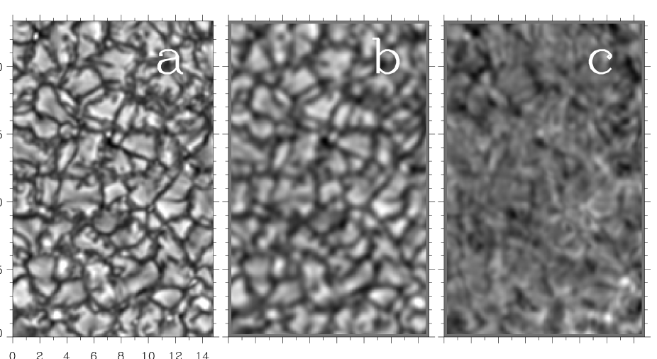
Figure 3: Example of reconstruction. a) Broad-band image (spatial resolution $\sim$ 0$\aas@@fstack{\prime\prime}$25). b) narrow-band continuum image (spatial resolution $\sim$ 0$\aas@@fstack{\prime\prime}$5). c) Intensity at the core of Fe i $\lambda$6302.5 Å. The axes are in arcsec.

Figure 3 shows a reconstruction. The axes are in arcsec so the FOV corresponds to 14″ $\times$ 23″. Figure 3a contains the broad-band image. The contrast of this image turns out to be 12.5% (by definition, the contrast is the standard deviation of the intensity in the image normalized to the mean intensity). Figure 3b shows the continuum intensity of the narrow-band reconstruction. In this case the contrast drops to some 7%. Figure 3c is the intensity at the core of Fe i $\lambda$6302.5 Å. Incidentally, the latter image provides yet another evidence supporting that the observations correspond to a very quiet Sun region. Network concentrations show up as conspicuous bright points at line core images (e.g., Sheeley 1967).

3.2 Stokes $I$ and Stokes $V$ profiles

The restoration process is carried out independently for the two images corresponding to the right and left circularly polarized beams $S_{1}$ and $S_{2}$. Once the restoration is completed, we compute the Stokes $I$ and Stokes $V$ profiles by adding and subtracting the two images at each wavelength,

$$V \propto S_{1}-S_{2},$$ (4)

$$I \propto S_{1}+S_{2}.$$ (5)

This task demands a careful superposition of the beams, which we carry out after sub-pixel interpolation. An example of a Stokes $I$ profile is included in Fig. 1. Several Stokes $V$ profiles are shown in Fig. 4.

Figure 4: Set of representative Stokes $V$ profiles of Fe i $\lambda$6302.5 Å. Despite the noise, deviations from the anti-symmetric shape are evident. (The large plus signs point out the origin of abscissae and ordinates.) We do not know which fraction of these asymmetries is real and which results from contamination with Stokes $I$. Wavelengths are in mÅ off line core $\lambda_{0}$. The polarization signals have been normalized to the continuum intensity $I_{c}$. The flux density assigned to each profile is included for reference.

3.3 Magnetograms and their calibration

Magnetic flux densities are computed starting from the the well-known magnetograph equation, which relates the circular polarization $V$ and the longitudinal component of the magnetic field $B$ (e.g., Unno 1956; Landi Degl’Innocenti 1992),

$$V(\lambda)=C(\lambda)\ B,$$ (6)

with

$$C(\lambda)=kg_{L}\lambda_{0}^{2}\frac{dI(\lambda)}{d\lambda}.$$ (7)

The symbols $\lambda$, $\lambda_{0}$ and $g_{L}$ stand for the wavelength, the central wavelength of the line, and the effective Landé factor, respectively. When Stokes $V$ and $I$ have the same units, the constant $k$ is equal to $-\leavevmode\nobreak\ 4.67\leavevmode\nobreak\ \cdot\leavevmode\nobreak\ 10^{-13}$ Å^-1 G^-1. We apply an independent calibration to each position of the field of view. First, the derivative of Stokes $I$ required to evaluate the calibration constant $C(\lambda)$ is computed numerically. Then, we select the wavelengths of the two extrema of the derivative, plus the two wavelengths immediately adjacent to each one of them. The selection renders six independent wavelength positions with $C(\lambda)\not=0$ where Eq. (6) could be applied to estimate $B$. Each wavelength gives a different value, so we chose a best estimate solving Eq. (6) by lest-squares. This procedure defines our estimate of the flux density $B_{\mathrm{eff}}$,

$$B_{\mathrm{eff}}=\frac{\sum_{j}V(\lambda_{j})C(\lambda_{j})}{\sum_{j}C^{2}(\lambda_{j})}.$$ (8)

The sum considers the six wavelengths $\lambda_{j}$ whose selection is described above (see also the square symbols in Fig. 15). Obviously, if the observed Stokes $I$ and $V$ profiles follow Eq. (6) then $B_{\mathrm{eff}}=B$. In practice this is not the case, and an extensive literature discusses various bias resulting from the break down of the magnetograph equation (refer to, e.g., Jefferies & Mickey 1991; Keller et al. 1994; Graham et al. 2002). Here we need to consider the main bias arising when the magnetic structure is much smaller than the resolution element, mostly filled by unmagnetized plasma. In this case,

$$B_{\mathrm{eff}}\simeq\alpha B,$$ (9)

$\alpha$ being the fraction of resolution element occupied by the otherwise uniform magnetic structure. According to Eq. (9), $B_{\mathrm{eff}}$ turns out to estimate the magnetic flux across the resolution element divided by the area of the resolution element (i.e., the magnetic flux density).

Two main sources of noise limit the precision of the flux density derived from Eq. (8). The measure is affected by the random noise of the Stokes $V$ spectra. We estimate its influence applying the law of propagation of errors (e.g., Martin 1971) to Eq. (8), i.e.,

$$\Delta B_{\mathrm{eff}}^{2}\simeq\sum_{j}\big{[}{\partial B_{\mathrm{eff}}}/{\partial V(\lambda_{j})}\big{]}^{2}\Delta V(\lambda_{j})^{2},$$

$$\leavevmode\nobreak\ \leavevmode\nobreak\ \leavevmode\nobreak\ \leavevmode\nobreak\ \leavevmode\nobreak\ \leavevmode\nobreak\ \leavevmode\nobreak\ \leavevmode\nobreak\ \simeq\Delta V^{2}/\sum_{j}C^{2}(\lambda_{j}),$$ (10)

where one assumes that the noise of the different wavelengths $\Delta V(\lambda_{j})$ is independent but has the same variance $\Delta V^{2}$. We have applied the previous equation to all individual profiles. The mean values of the errors are

$$\Delta B_{\mathrm{eff}}\simeq 23\ {\rm G\ for\ Fe}\ {\sc I}\ \lambda 6301.5\ {\rm\AA},$$ (11)

$$\Delta B_{\mathrm{eff}}\simeq 17\ {\rm G\ for\ Fe}\ {\sc I}\ \lambda 6302.5\ {\rm\AA}.$$ (12)

The $\Delta V$ required to evaluate Eq. (10) was set to $5\times 10^{-3}\leavevmode\nobreak\ I_{c}$, $I_{c}$ being the continuum intensity. This figure was estimated from the standard deviation of $V$ as a function of $\lambda$ when $B_{\mathrm{eff}}$ becomes zero. Explicitly, the standard deviation of all observed spectra was represented versus $B_{\mathrm{eff}}$. Such scatter plot gives a non-zero Stokes $V$ standard deviation for $B_{\mathrm{eff}}=0$. This value is used for $\Delta V$.

A second source of error affecting $B_{\mathrm{eff}}$ is due to the contamination of the polarization signals with intensity. Following the procedure described in Sect. 3.2, spatially restored spectra proportional to $I+V$ and $I-V$ are obtained for each point on the solar surface,

$$S_{1}= f_{1}\ (I+V)/2,$$ (13)

$$S_{2}= f_{2}\ (I-V)/2.$$ (14)

The circular polarization is estimated by subtracting them out (Eq. (5)),

$$\widehat{V}=S_{1}-S_{2}.$$ (15)

This would yield the true solar $V$ signal if $f_{1}=f_{2}=1$. However, due to the uncertainties of the reduction procedure (e.g., normalization to the continuum intensity, insufficient flatfielding, non-linearities of the cameras, instrumental polarization induced by the telescope, etc), $f_{1}\not=f_{2}$ and $\widehat{V}$ is contaminated by the intensity profile $I$,

$$\widehat{V}\simeq V+{{f_{1}-f_{2}}\over{2}}\ I.$$ (16)

Since $V\ll I$, the crosstalk with intensity seriously threatens the polarimetric accuracy of the measurements. Equation (8) was devised to automatically correct for this crosstalk, at least to first order. One can estimate the residual error due to crosstalk with intensity as follows. Equations (8) and (16) lead to

$$\Delta B_{\mathrm{eff}}=B_{\mathrm{eff}}-B_{\mathrm{eff0}}={{f_{1}-f_{2}}\over 2}\Delta B,$$ (17)

with $B_{\mathrm{eff0}}$ the flux density to be retrieved if there were no crosstalk, and $\Delta B$ characterizing the bias,

$$\Delta B=\frac{\sum_{j}I(\lambda_{j})C(\lambda_{j})}{\sum_{j}C^{2}(\lambda_{j})}.$$ (18)

Note that $\Delta B$ only depends on the intensity. We have estimated its value using a mean quiet Sun profile smoothed and sampled to mimic the observational procedures: $\Delta B\sim\thinspace 150$ G for Fe i $\lambda$6301.5 Å and $\sim\thinspace 120$ G for Fe i $\lambda$6302.5 Å. Keeping in mind that the crosstalk $(f_{1}-f_{2})/2$ has to be smaller than a few per cent (otherwise the contamination would exceed the real Stokes $V$ signals), the bias induced by the crosstalk with intensity $\Delta B\ (f_{1}-f_{2})/2$ is at most a few G. This figure is negligibly small compared to the error produced by random noise (Eq. (12)). Should we had used a different procedure to measure $B_{\mathrm{eff}}$, the bias would be unbearable. For example, using only one wing of the line $\Delta B\sim 3.5\times 10^{3}$ G for Fe i $\lambda$6301.5 Å, which renders $\Delta B_{\mathrm{eff}}\simeq 70$ G for a 2% crosstalk ($[f_{1}-f_{2}]/2=2\,\cdot\,10^{-2}$). The huge difference with respect to our procedure is due to the cancellation of positive and negative contributions in Eq. (18) when the two wings are considered.

3.4 Velocities

A brief discussion on the velocities associated with the magnetic signals is included in Sect. 4.3. These velocities are computed as the wavelength of the minimum of a parabola that fits the core of the Stokes $I$ profiles. The zero of the velocity scale is set by the mean velocity across the full FOV, so it is affected by the convective blueshift.

3.5 Time series

We analyze the time variation of the magnetic signals (Sect. 5). In order to produce a movie from the individual speckle reconstructed magnetograms, the individual snapshots of the series were co-aligned allowing for a global shift among them. Such displacement is computed by minimizing the difference between the successive broad-band images of the time series. The mean broad-band image of the series constructed in this way has a contrast of the order of 7%. This figure has to be compared to the contrast of the best image in the series, which is some 12.5% (Sect. 3.1).

4 Results

4.1 Mean flux density of the magnetograms

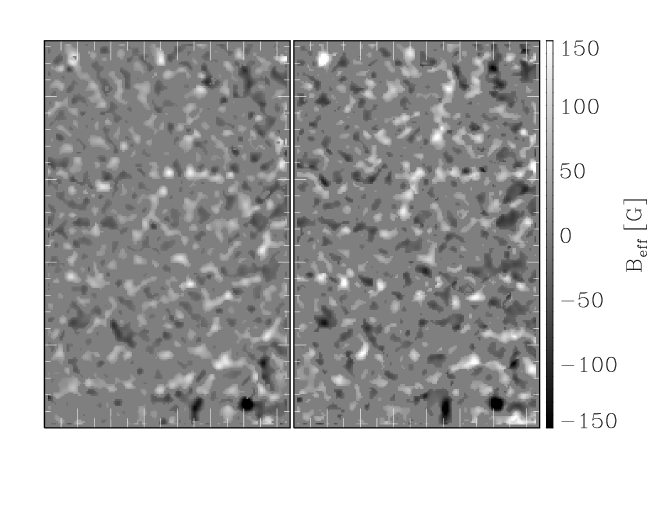
Figure 5: Magnetograms from Fe i $\lambda$6302.5 Å (left) and Fe i $\lambda$6301.5 Å (right). The signals below the noise level are set to zero. Dark and light represent different polarities, as coded in the vertical bar. Tick marks are separated by 1 arcsec.

Figure 5 presents two simultaneous magnetograms taken in the two iron lines. (They correspond to the snapshot of the time series having the best angular resolution, which is the one that we analyze in detail.) They exhibit a salt and pepper pattern with patches of opposite polarity in close contact. Approximately 60 % of the FOV contains polarimetric signal above noise in one of the spectral lines. This large area coverage, together with the fair magnetic sensitivity of the measurements, yields more magnetic flux than any previous observation of the photospheric IN magnetic fields (Sect. 6.2). In order to quantify the amount of flux, we have evaluated the mean unsigned flux density in the observed region $\overline{|B_{\mathrm{eff}}|}$,

$$\overline{|B_{\mathrm{eff}}|}\equiv\frac{1}{\tilde{N}}\sum_{i}|B_{\mathrm{eff}}^{i}|,$$ (19)

where the sum includes only those pixels with signal above noise in one of the spectral lines, and $\tilde{N}$ represents the total number of pixels in the FOV. ($\overline{|B_{\mathrm{eff}}|}$ is the average $|B_{\mathrm{eff}}|$ over the FOV once signals below noise are set to zero.) The result of the computation yields

$$\overline{|B_{\mathrm{eff}}|}=\cases{21\leavevmode\nobreak\ {\rm G},&for {Fe {i}}\leavevmode\nobreak\ $\lambda$6301.5\leavevmode\nobreak\ \AA;\cr 17\leavevmode\nobreak\ {\rm G},&for {Fe {i}}\leavevmode\nobreak\ $\lambda$6302.5\leavevmode\nobreak\ \AA.}$$ (20)

These mean flux densities are weakly affected by the noise of the individual $B_{\mathrm{eff}}^{i}$, since $\overline{|B_{\mathrm{eff}}|}$ results from the average of thousands of individual pixels. The fact that we average absolute values and the use of a threshold do not modify this argument. We carried out Monte-Carlo simulations that show the robustness of the estimates (20). Using the full magnetograms (including effective flux densities below the noise), we added random Gaussian noise according to our estimate of the noise level (Eq. (12)). The application of the definition (19) to different realizations of magnetograms with mock noise renders the same mean flux densities within a fraction of one G.

We have also computed the mean signed magnetic flux density for the magnetograms in Fig. 5 (with a definition similar to the unsigned flux Eq. (19) but using $B_{\mathrm{eff}}^{i}$ instead of $|B_{\mathrm{eff}}^{i}|$). It turns out to be,

$$\overline{B_{\mathrm{eff}}}=\cases{+2\leavevmode\nobreak\ {\rm G},&for {Fe {i}}\leavevmode\nobreak\ $\lambda$6301.5\leavevmode\nobreak\ \AA;\cr+3\leavevmode\nobreak\ {\rm G},&for {Fe {i}}\leavevmode\nobreak\ $\lambda$6302.5\leavevmode\nobreak\ \AA.}$$ (21)

Note that $\overline{B_{\mathrm{eff}}}\leavevmode\nobreak\ \ll\leavevmode\nobreak\ \overline{|B_{\mathrm{eff}}|}$, which probably constrains the physical mechanisms responsible for the observed magnetic structure (they have to create large unsigned magnetic fluxes and, simultaneously, low signed fluxes). This constraint is probably even more severe than the values inferred from combining Eqs. (20) and (21), since we cannot discard systematic errors of a few G affecting $\overline{B_{\mathrm{eff}}}$ (see, e.g., Sect. 3.3).

4.2 Magnetic field strengths and filling factors

The polarization signals obtained from the two spectral lines are correlated (see Fig. 5). However, the magnitude of the effective flux density of Fe i $\lambda$6301.5 Å, $B_{\mathrm{eff}}(6301)$, is systematically larger than the effective field derived using Fe i $\lambda$6302.5 Å, $B_{\mathrm{eff}}(6302)$. The difference is inferred from mean fluxes (e.g., from Eq. (20)), since the noise prevents conclusions based on individual measurements. We calculate the mean excess of $B_{\mathrm{eff}}(6301)$ with respect to $B_{\mathrm{eff}}(6302)$ by means of a lest-squares fit that accounts for the errors of both $B_{\mathrm{eff}}(6301)$ and $B_{\mathrm{eff}}(6302)$. We only consider flux densities above noise. Our best estimate is

$$B_{\mathrm{eff}}(6301)/B_{\mathrm{eff}}(6302)\simeq 1.25\pm 0.14.$$ (22)

The error bar corresponds to the standard 68% confidence level, and it is worked out in Appendix A, where we also reject the hypothesis $B_{\mathrm{eff}}(6301)=B_{\mathrm{eff}}(6302)$ with high confidence. The 25% systematic difference can be easily interpreted if the intrinsic magnetic field strengths of the structures that give rise to the signals in the magnetograms exceeds 1 kG. Should the magnetic fields be intrinsically weak (say, a few hundred G), the magnetograph equation holds since the basic conditions for the approximation to be valid are satisfied. First, the Zeeman splittings of both Fe i $\lambda$6301.5 Å and Fe i $\lambda$6302.5 Å are smaller than the Doppler width of the lines. Second, the magnetic fields are dynamically weak, and they cannot modify the thermodynamic conditions with respect to those in the un-magnetized atmosphere. Even if one does not spatially resolve the magnetic structures, the calibration constants derived from the observed Stokes $I$ are valid, Eq. (9) applies, and $B_{eff}(6301)/B_{eff}(6302)=1$. Consequently, the fact that the observed ratio (22) differs from one implies the existence of strong fields. These qualitative arguments, in the spirit of the line-ratio method of Stenflo (1973), were already put forward by Socas-Navarro & Sánchez Almeida (2002). The arguments can be made quantitative computing the ratio of effective field strengths in different model atmospheres whose intrinsic field strengths are known. We have carried out such calibration, and the details are given in Appendix B. The ratio of effective magnetic field strengths versus the intrinsic field strength is computed in a variety of atmospheres (Fig. 14). Two main results arise from this calibration:

• The observed ratio (22) indicates the existence of magnetic fields larger than 1 kG in the photospheric layers where the observed polarization is formed. More precisely $900\leavevmode\nobreak\ {\rm G}\leavevmode\nobreak\ \leq\leavevmode\nobreak\ B\leavevmode\nobreak\ \leq\leavevmode\nobreak\ 1600\leavevmode\nobreak\ {\rm G}$ when $1.1\leavevmode\nobreak\ \leq\leavevmode\nobreak\ B_{eff}(6301)/B_{eff}\leavevmode\nobreak\ (6302)\leavevmode\nobreak\ \leq\leavevmode\nobreak\ 1.4$.

• The fact that the ratio (22) corresponds to kG fields is almost insensitive to the details of the model atmosphere. This property was expected according to the qualitative arguments given above.

Note that these conclusions do not discard the existence of sub-kG magnetic field strengths in our data. Despite the fact that the characteristic field strength seems to be kG, the scatter among the individual ratios is very large. Consequently, there are many individual points whose ratio can be unity or smaller which, according to the calibration above, implies sub-kG field strengths.

Structures with intrinsic kG magnetic field strength showing 20 G flux density have to occupy only a small fraction of the solar surface. The simple 2-component model allows to estimate the area coverage or filling factor. The filling factor is just the ratio between effective and intrinsic field strengths (Eq. (9)). If $B\sim$ 1 kG then

$$\alpha\sim B_{\mathrm{eff}}/B\sim 20\leavevmode\nobreak\ {\rm G}/1000\leavevmode\nobreak\ {\rm G}\sim 0.02.$$ (23)

Only 2% of the solar surface produces the observed signal. We observe them to cover 60% of the FOV because of the limited spatial resolution of the observations. One can also employ the same order-of-magnitude calculation to estimate the size $l$ of the magnetic concentrations. If $M$ magnetic concentrations occupy a resolution element of size $L$, then

$$\alpha\sim(l/L)^{2}M,$$ (24)

which, together with Eq. (9), renders

$$l\sim L\sqrt{B_{\mathrm{eff}}/(M\,B)}\sim\cases{75\leavevmode\nobreak\ \mathrm{km}&for M=1;\cr 25\leavevmode\nobreak\ \mathrm{km}&for M=10;\cr 10\leavevmode\nobreak\ \mathrm{km}&for M=50.}$$ (25)

We use $L=0\aas@@fstack{\prime\prime}5\equiv 363$ km, $B=1$ kG, and $B_{\mathrm{eff}}=40$ G, the latter being the typical value of the signals above noise in the magnetograms of Fig. (5).

4.3 Spatial distribution and brightness of elements with magnetic signal

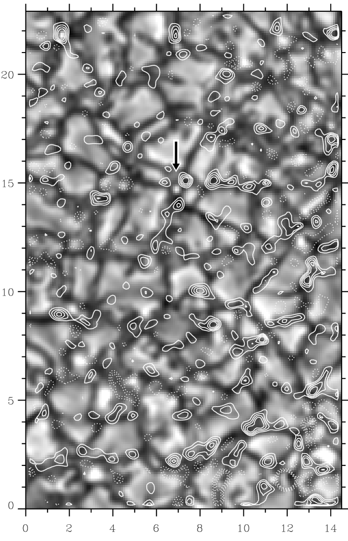
Figure 6: Speckle reconstructed broad-band image overlaid with the magnetogram of Fe i $\lambda$6302.5 Å with contours at $B_{\mathrm{eff}}=$ $\pm 30$, $\pm 50$, $\pm 70$, and $\pm 90$ G. The solid and dotted contours indicate opposite polarities. The distance between tick-marks is 1 arcsec, as indicated by the labels of the axes. The arrow points out an isolated bright point without associated polarization signal.

Figure 6 shows the speckle reconstructed broad-band image and, overlaid to it, the Fe i $\lambda$6302.5 Å magnetogram. Most of the magnetic fields are located in intergranular lanes. This tendency has been observed before (Lin & Rimmele 1999; Lites 2002; Socas-Navarro 2003) and is expected from numerical simulations of magneto-convection (e.g., Weiss 1978; Cattaneo 1999; Vögler & Schüssler 2003). However, some magnetic field signals are also found in granules, in agreement with the observations of Stolpe & Kneer (2000) and Koschinsky et al. (2001). This bias of the magnetic signals towards intergranules is also evident from the inspection of Fig. 7, which contains histograms of the distributions of continuum intensities and velocities. The figure displays both, pixels with signals above noise (the solid lines), and below noise (the dotted lines). Some 65% of the magnetic signals of Fe i $\lambda$6302.5 Å are darker than the mean intensity, which indicates association with intergranular lanes. On the other hand, 60 % of these pixels present redshifts, which correspond to downflows in the solar atmosphere and therefore trace intergranules. The histograms based on Fe i $\lambda$6301.5 Å present similar trends.

Figure 7: Histograms of continuum intensities (a) and velocities (b) for pixels with magnetic fields above the noise level (the solid lines) and below the noise level (the dotted lines). The intensities refer to the mean intensity, and the average velocity over the FOV is set to zero. We adopt the convention that redshifts are positive. The histograms correspond to Fe i $\lambda$6302.5 Å.

The strong signals in the magnetograms show a pattern whose characteristic size corresponds to the mesogranular convective cells, i.e., with a spatial scale between 5 and 10 arcsec (Fig. 8). Mesogranulation has been detected in velocity (e.g., November et al. 1981) and intensity (e.g., Deubner 1989), and it is also recovered from numerical simulations of magneto-convection (e.g., Cattaneo et al. 2001). However, to the authors’ best knowledge, this is the first clear detection in polarization. (For another observation suggestive of mesogranulation in polarized light, see Trujillo Bueno 2003, Fig. 4.) Figure 8, left, portraits the magnetogram of the region except that only fluxes above 50 G have been represented. One can guess a cellular pattern with a scale larger than the granules but still smaller than the supergranulation (the latter with a scale larger than the FOV). This pattern is long-lived since it shows up in the mean magnetogram of our 17 min time sequence (Fig. 8, right; see also Sect. 5). Our finding should be regarded as an additional observational proof for the existence of the mesogranular convective scale.

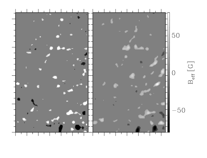
Figure 8: Left: magnetogram of the region showing only strong signals, explicitly, flux densities above 50 G. The rest is set to zero. Note the regular pattern with a size similar to the 5-10″scale of the mesogranulation (tick-marks correspond to 1 arcsec). Right: mean magnetogram of the time series, which still shows a pattern similar to that of the single snapshot. In this case we set to zero those flux densities below 25 G .

We have found magnetic structures that typically harbor kG magnetic fields. According to the common wisdom, they should be bright in broad-band images. The presence of a kG field reduces the density of the magnetized plasma and thus lowers the opacity with respect to the ambient atmosphere. One sees deeper through the magnetized plasma which (usually) means observing hotter layers that produce more light (often called hot-wall effect; Spruit 1976). Except for a few cases (e.g., bright points at [1$\aas@@fstack{\prime\prime}$5, 22″], [12″, 1″], or [8″, 10″] in Fig. 6), we do not see bright points associated with the magnetic signals. Moreover, the intergranules having magnetic signals do not seem to be brighter than those without them (see the histograms in Fig. 9).

Figure 9: Distribution of broad-band intensities in intergranules with and without magnetic field. Intergranules are selected as those points with intensity smaller that 90% of the mean intensity. The two types of line distinguish the histograms obtained for points with magnetic field above the noise (the solid line) and those with no detected signals (the dashed line). There is no obvious difference. The histograms provide the percentage of points in each bin.

This seeming inconsistency between the expected but unobserved brightness may not be real. There are several ways to reconcile the observations with the current paradigm, for example,

• the sizes of the individual kG magnetic concentrations (see Eq. (25)) are small compared with the sizes of intergranular lanes. Even very bright but small magnetic structures may lead to dark signals when observed with the kind of (good but still insufficient) angular resolution of the broad-band image (see Title & Berger 1996).

• If the temperature of the intergranules is low enough, the expected reduction of opacity associated with the presence of kG magnetic fields may not produce a bright structure. The depression of the observed layers by a few tens of km may not be enough to reach temperatures larger than those of the mean un-depressed photosphere (see, e.g., Stein & Nordlund 1998, Fig. 14).

• Due to a yet unknown physical process, there may be a tendency for the magnetic structures to stay in the darkest intergranular lanes (e.g., they accumulate in the strong downflows that tend to be particularly dark.)

Note, finally, that the signals in Fig. 6 cannot be misidentified network magnetic concentrations, since they occur at a characteristic scale much smaller than the supergranulation.

4.4 Stokes $V$ asymmetries

The Stokes $V$ profiles observed in quiet network and inter-network regions show large deviations from the anti-symmetric shape (Sánchez Almeida et al. 1996; Grossmann-Doerth et al. 1996; Sigwarth et al. 1999; Sánchez Almeida & Lites 2000). These so-called asymmetries carry meaningful information on the structure of the magnetic atmosphere (e.g., Sánchez Almeida 1998, and references therein). It would have been desirable studying the asymmetries of our profiles in some detail. However, the Stokes $I$ to $V$ contamination described in Sect. 3.3, Eq. (16), masks the real asymmetries in a significant way, and we refrain from analyzing them. Once this caveat has been explicitly pointed out, we also would like to mention that asymmetric Stokes $V$ profiles are found everywhere in the FOV. In particular, we observe Stokes $V$ profiles with only one lobe and profiles with three lobes (see Fig. 4).

5 Temporal evolution

The duration (17 min) and cadence (50 s) of the series of magnetograms are far from optimum to allow a detailed study of the temporal evolution of the structures. In addition, the polarization signals are close to the noise level, and the seeing conditions vary along the sequence. These two factors induce spurious time variations which complicate the analysis. Despite these drawbacks, several conclusions on the time evolution of the magnetic signals can safely be drawn. We extracted them from the inspection of the sequence of magnetograms re-centered as described in Sect. 3.5.

Many individual features maintain their identity in successive time steps of the series (see Fig. 10, where time increases from top to bottom and from left to right). In fact, some of the signals live longer than the total time span, as it is proven by Fig. 8 where the strongest signals in the mean magnetogram of the series resemble those of any individual snapshot.

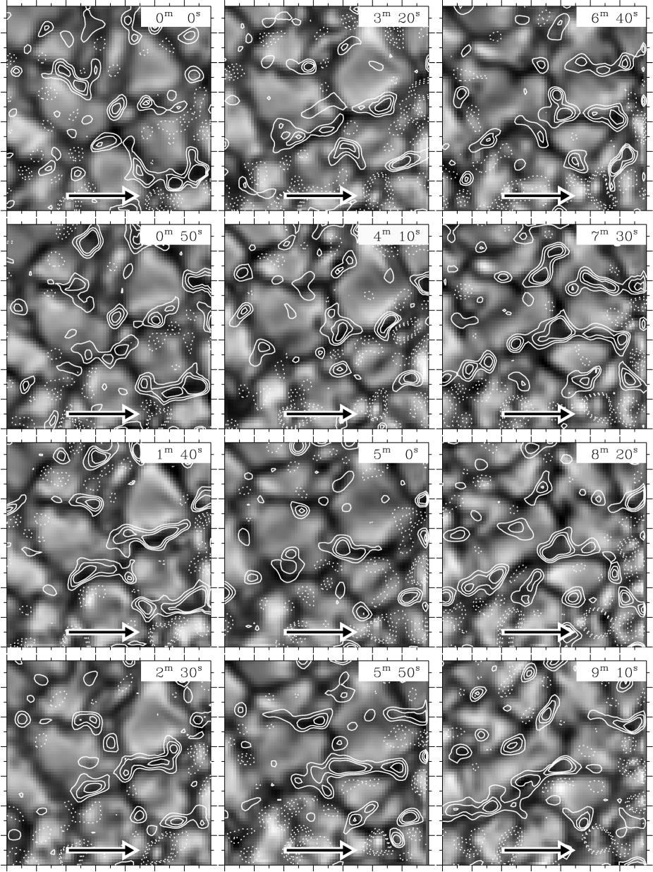
Figure 10: Temporal evolution. Magnetograms overlapped to intensity images as in Fig. 6 but for a sub-field of 7″$\,\times\,7$″. Time increases from top to bottom and from left to right. The different images are consecutive snapshots of the series separated by 50 s (see the labels on the images). The arrow points out a specific region dominated by a magnetic concentration of negative polarity that interacts with positive polarity patches and, possibly, eats them away.

This mean magnetogram has been computed as a weighted average of the individual magnetograms of the series, with the weights given by the inverse of the squared noise of the magnetograms (Eq. 12). In order to quantify the fraction of unsigned flux that survives more than the time-span, we have computed the unsigned flux density for signals above noise level in the mean magnetograms. They turn out to be,

$$\overline{|B_{\mathrm{eff}}|}=\cases{13\leavevmode\nobreak\ {\rm G},&for {Fe {i}}\leavevmode\nobreak\ $\lambda$6301.5\leavevmode\nobreak\ \AA;\cr 9\leavevmode\nobreak\ {\rm G},&for {Fe {i}}\leavevmode\nobreak\ $\lambda$6302.5\leavevmode\nobreak\ \AA,}$$ (26)

They represent 60% of the flux density in the best individual magnetogram (Eq. (20)). It is tempting to interpret this figure as the fraction of IN magnetic structures that live longer than 17 min. However, the interpretation is not so straightforward since we detect polarization signals rather than magnetic structures. Seemingly long-lived signals may not necessarily correspond to stable magnetic structures. Numerical simulations of quiet Sun magneto-convection show persistent downdrafts that continuously gather magnetized plasma in specific locations (e.g. Cattaneo 1999; Emonet & Cattaneo 2001). The plasma sinks down and disappears along the downdrafts, and it is continuously replaced by new plasma. The system of persistent downdrafts outlines mesogranular cells, which live much longer than the individual magnetic structures. This theoretical scenario is consistent with the observed magnetograms and, in particular, with the existence of a long lasting polarization pattern that we have already associated with the mesogranulation (see Sect. 4.3). Consequently, the existence of signals in the mean magnetogram is interpreted here as a proof of the temporal coherence of the mesogranular pattern, rather than the persistence of individual magnetic concentrations.

On top of the rather stable pattern described above, large variations of the magnetic signals occur between snapshots (Fig. 10). Some polarization signals migrate following the granular motions to remain in the intergranular spaces. There are places where opposite polarities approach each other and seem to (partly) cancel out; the arrow in Fig. 10 indicates a negative polarity patch (dotted line) that interacts, and possible eats away, neighboring positive polarity contours (compare the snapshots at 0${}^{\mathrm{m}}\,0^{\mathrm{s}}$ and 4${}^{\mathrm{m}}\,10^{\mathrm{s}}$). More often signals grow and fade with no obvious interference with patches of opposite polarity. As we pointed out above, these variations only trace changes in the polarization signals, which do not necessarily imply the evolution of the magnetized plasma. Actually, one may have large variations of polarization without substantial changes of the underlying magnetic structure. For example, Sánchez Almeida (2000) describes how the polarization of kG magnetic concentrations can vanish upon a small increase of the field strength. This effect is mentioned here because it may be responsible for the lack of magnetic signal associated to the bright point indicated by an arrow in Fig. 6. Subsequent magnetograms of the series show that this bright point is co-spatial with polarization signals.

The mean unsigned flux density is only slightly different for the different snapshots of the series. The standard deviation of these changes is some 10% for Fe i $\lambda$6302.5 Å, whereas it reaches 20% for Fe i $\lambda$6301.5 Å. There is a tendency for the snapshots of largest continuum contrast to have the largest flux densities.

6 Consistency of the results

The unsigned flux densities that we find are larger than the values found hitherto. The purpose of this section is to spell out arguments that support the reliability of our results. The magnetograms have self-consistency since independent parts of the data set provide similar results. They are also consistent with previous observations having different sensitivities and angular resolutions, once these differences are properly taken into account. Finally, the signals meet several theoretical prejudices which are independent of the observation. In particular, the signals appear in the intergranular lanes and show a conspicuous and stable mesogranular pattern.

6.1 Self-consistency

We have a time sequence of magnetograms taken in two different spectral lines. Magnetograms differing in time or spectral line are independent, and they can be analyzed independently to check the self-consistency of various results. We have identified the following properties of the data set that support the internal agreement between independent subsets,

• the simultaneous magnetograms obtained from the two lines are very similar (Fig. 5).

• Many patches in the magnetograms are larger than the resolution of the observation, implying a spatial coherence of the signals difficult to ascribe to noise.

• The signals are co-spatial with the dark intergranular lanes (Sect. 4.3). Again, this relationship is difficult to explain as due to noise. One might suspect that the misalignment of the two circularly polarized beams subtracted to determine Stokes $V$ creates false polarization signals. This contamination would be maximum where the spatial gradients in intensity or velocity are maximum (e.g., Lites 1987). The maximum gradients occur in the transitions between granules and intergranules, which is not where the detected signals are. We have checked that the scatter plots of polarization signals versus spatial gradients show no obvious correlation.

• Many polarization patches maintain their identity in several successive magnetograms of the series. In particular, the mean magnetogram retains some 60 % of the peak flux density (Eq. (26)), a fact once again difficult to explain as due to noise. Should the signals be noise, the mean magnetogram would show signals much smaller than that of individual frames (i.e., only $\sim 1/\sqrt{20}\sim 20$ % of the individual signals).

6.2 Comparison with other measurements

Our observations differ in angular resolution and sensitivity from previous measurements. These factors have to be taken into account before they can be properly compared. We have to cut down the resolution of the magnetogram and then change the sensitivity of the measurement.

The speckle reconstructed images can be regarded as the true solar image down to the cutoff frequency. In the case of our magnetograms, the cutoff corresponds to a period of 0$\aas@@fstack{\prime\prime}$5 (see Sect. 3.1, Fig. 2). We model the effect of seeing on the measured images by convolving the speckle reconstructed images with a Gaussian point spread function. This smoothing is carried out independently for each single wavelength. Then the different wavelengths are combined and processed to get magnetic flux densities in the same way as the original images. The FWHM of the Gaussian kernel is used to quantify the seeing. Figure 11 shows how the magnetograms (left) and broad-band intensities (right) appear under various seeing conditions: 0$\aas@@fstack{\prime\prime}$3, 0$\aas@@fstack{\prime\prime}$5, 1″  and 2″. The field of view of the section of the magnetogram that we present is only 7″$\,\times\,$7″. Even when the seeing is fair (1″), only traces of the signals in the speckle reconstructed images are left.

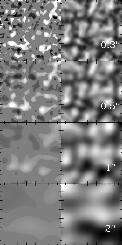
Figure 11: Magnetograms (left) and continuum intensities (right) for different seeing conditions as indicated by the insets. All magnetograms have the same scale, which saturates at -60 G and 60 G. The field of view is only 7″$\,\times\,$7″.

The unsigned flux density that survives a given seeing is shown in Fig. 12.

Figure 12: Mean unsigned Fe i $\lambda$6302.5 Å flux density that remains in the magnetograms when observed with the seeing given in the abscissa. If all signals above noise are considered, one is left with the solid line. If only signals above 20 G are considered, then the reduction is much more severe as represented by the dashed line. Finally, when very large flux densities are considered (signals larger than 100 G) almost no signal remains (the dotted line).

It contains the signals above three different levels of noise (or different sensitivities): 100 G, 20 G and the actual noise in the magnetograms. The decrease of angular resolution reduces the signals due to cancellation between close opposite polarities. For an angular resolution corresponding to 1″($\equiv 0.75$ Mm), the mean unsigned flux density become of the order of 7 G. This value agrees with previous determinations based on scanning spectro-polarimeters that reach 1″ resolution (Sánchez Almeida & Lites 2000 and Lites 2002 obtain some 10 G). Sánchez Almeida et al. (2003) collect different values from the literature, showing a magnitude and trend that resembles the solid line in Fig. 12. In particular, Wang et al. (1995) point out a flux density of 1.65 G for a 2″ resolution, which is not far from the value that remains in our magnetograms for this resolution (some 2.5 G; Fig. 12). On the other hand, magnetograms with an angular resolution similar to those presented here exist in the the literature (Keller 1995; Koschinsky et al. 2001; Berger & Title 2001). However, they have a noise level between 50 G and 150 G, which exceeds the limit required to detect most of the signals in our magnetograms. This lower sensitivity can easily explain why the IN signals that we detect have been missed so far. Figure 12 shows that the mean flux density drops below 1-2 G when only signals above 100 G are considered. In short, our magnetograms are consistent with previous observations when the limitations of angular resolution and sensitivity are taken into account.

We find imbalance between the two polarities so that there is a net magnetic flux across the region (Eq. (21)). We do not claim that the effect is real since it is at the level of systematic effects that may be important (see Sect. 3.3). However, imbalances of similar magnitude have been found in the IN by other authors (see Lites 2002), and consequently, the imbalance may be true. If so, it would be one more aspect of our observation being consistent with previous measurements of IN field properties.

7 Conclusions

We have obtained a time sequence of speckle reconstructed quiet Sun magnetograms showing magnetic signals that cover 60% of an Intra-Network region (Fig. 6). The signals appear as patches of opposite polarity often located close to each other. The structures are not evenly spread out, but they tend to accumulate in the intergranular lanes. Those signals of large flux density trace a network whose scale is larger than the granules and smaller that the supergranules. We associate this network with the mesogranulation, difficult to observe in velocity and intensity but very conspicuous in polarization (Fig. 8). The mesogranular pattern lives longer than the time span of the series (17 min).

The effective flux density deduced from Fe i $\lambda$6301.5 Å is systematically larger than the flux density of Fe i $\lambda$6302.5 Å (Eq. (22)). We interpret this difference as due to the presence of kG field strengths in the underlying magnetic structures. These field strengths saturate, differently, the polarization signals of the two spectral lines. The inference of kG, however, does not rule out that weaker field strengths are responsible for some of the observed signals (see Sect. 4.2). Since the flux density is proportional to both the field strength and the filling factor, we are forced to conclude that the true magnetic concentrations producing the polarization cover only a small fraction of the surface; some 2%.

The magnetic signals that we observe meet several theoretical prejudices: they appear in intergranular lanes, trace mesogranulation, vary in short timescales, and have complex topology with opposite polarities in contact. These properties are easy to interpret as the result of the interaction between granular convection and magnetic fields, no matter whether the fields are produced by a local dynamo (Petrovay & Szakaly 1993; Cattaneo 1999; Emonet & Cattaneo 2001), a global dynamo (Stein & Nordlund 2002), or they represent re-processed materials left by old active regions (e.g., Schüssler 2003; Vögler & Schüssler 2003). There are other observational properties which do not accommodate so easily within the existing paradigms. The field strengths are typically kG, so a process has to concentrate the fields to this level. The convective collapse (Parker 1978; Spruit 1979), devised for network magnetic concentrations, may have difficulty to concentrate the low magnetic flux features that we detect (see Sánchez Almeida 2001). Yet another observational constraint difficult to satisfy is the large difference between the signed and unsigned flux densities. Whatever physical mechanism generates the observed fields, it has to produce a distribution of magnetic field whose mean flux is 10 times smaller than the local fluctuations of flux.

Sánchez Almeida et al. (2003) compile values for the mean unsigned flux density of the IN fields measured by different authors. They show a tendency to increase as the angular resolution improves, but none of them exceeds 10 G. Our magnetograms contain more magnetic flux than the values reported hitherto. We detect more polarization signals probably due to the unique combination of high spatial resolution and good sensitivity. The magnetic flux detected in the IN critically depends on the polarimetric sensitivity and the angular resolution. If these factors are properly taken into account, our estimates of unsigned flux density are compatible with the previous measurement.

We find evidence that our angular resolution and sensitivity do not suffice to detect all the magnetic flux existing in the quiet Sun. The flux density in the magnetograms drops off upon artificial reduction of polarimetric sensitivity or spatial resolution (Fig. 12). The extrapolation of this trend predicts a notable increase of signals upon improvement of the observational limitations. On the other hand, we have concluded that the observed signals are tracing kG magnetic fields. There are sensible theoretical arguments pointing out that the spectral lines used to measure are biased towards these kG fields (Sánchez Almeida & Lites 2000; Socas-Navarro & Sánchez Almeida 2003). In other words, magnetic concentrations of sub-kG field strength could have been easily overlooked by our magnetograms. These and other reasons suggest that the IN flux detected so far should be regarded as a lower limit to the true flux. Thus any effort to improve the sensitivity and/or angular resolution is likely to be rewarded with new magnetic flux.

Appendix A Ratio $B_{\mathrm{eff}}(6301)/B_{\mathrm{eff}}(6302)$

We want to estimate the typical ratio of effective magnetic fluxes taking into account that (a) the measured magnetic fluxes of the two lines have errors, and (b) these errors are not negligible. We invoke several results from statistics, which can be found in standard textbooks (e.g., Martin 1971). For the sake of conciseness, and only in this Appendix, the following notation is employed

$$B_{1i}\equiv B_{\mathrm{eff}}(6301){\mathrm{\leavevmode\nobreak\ in\leavevmode\nobreak\ the{\it\leavevmode\nobreak\ i-th}\leavevmode\nobreak\ pixel}},$$ (27)

$$B_{2i}\equiv B_{\mathrm{eff}}(6302){\mathrm{\leavevmode\nobreak\ in\leavevmode\nobreak\ the{\it\leavevmode\nobreak\ i-th}\leavevmode\nobreak\ pixel}}.$$ (28)

The fluxes observed in each pixel have true values, $B_{1i}^{0}$ and $B_{2i}^{0}$, plus noise, $\Delta B_{1i}$ and $\Delta B_{2i}$,

$$B_{1i}= B_{1i}^{0}+\Delta B_{1i},$$ (29)

$$B_{2i}= B_{2i}^{0}+\Delta B_{2i}.$$ (30)

We assume the noise of the two fluxes to be independent, since they come from separate data. We also assume a linear relationship between the true fluxes,

$$B^{0}_{1i}=m\,B_{2i}^{0},$$ (31)

being $m$ the ratio that we want to estimate. The above expression, combined with Eq. (30), renders a linear relationship between the two observables $B_{1i}$ and $B_{2i}$ that explicitly includes noise,

$$B_{1i}=mB_{2i}-m\Delta B_{2i}+\Delta B_{1i}.$$ (32)

As usual, $m$ is determined by means of a least-squares fit. We chose to minimize the merit function

$${\rm X}^{2}(m)=\Large\sum_{i=1}^{N}{{(B_{1i}-mB_{2i})^{2}}\over{\sigma^{2}_{1i}+m^{2}\sigma_{2i}^{2}}},$$ (33)

where $\sigma^{2}_{1i}$ and $\sigma_{2i}^{2}$ are the variances of the probability density functions describing the noise $\Delta B_{1i}$ and $\Delta B_{2i}$,

$$\sigma^{2}_{1i}\equiv V\{\Delta B_{1i}\}=V\{B_{1i}\},$$ (34)

$$\sigma^{2}_{2i}\equiv V\{\Delta B_{2i}\}=V\{B_{2i}\},$$ (35)

whose expectation values are assumed to be zero,

$$E\{\Delta B_{1i}\}=E\{\Delta B_{2i}\}=0.$$ (36)

(The symbol $V\{\leavevmode\nobreak\ \}$ stands for the variance of a random variable, and it should not be confused with the Stokes $V$ parameter.) $N$ in Eq. (33) represents the number of pixels used in the estimate. This particular merit function has been selected because it presents several practical advantages:

• $E\{B_{1i}-mB_{2i}\}=0$, $V\{B_{1i}-mB_{2i}\}=\sigma^{2}_{1i}+m^{2}\sigma_{2i}^{2}$, and so, invoking the central limit theorem, each term of the definition (33) is the square of a random variable distributed according to a n(0,1) (i.e., a normal distribution with mean of zero and variance of one). Should the noise of different pixels be independent, the random variable ${\rm X}^{2}$ follows a $\chi^{2}$ distribution, which makes it easy setting confidence intervals and performing statistical tests (see below).

• The ratio of flux densities derived from the fit does not depend on whether we estimate $m$ or $m^{-1}$, i.e., on whether we start up from the relationship (31) or its inverse $B^{0}_{2i}=m^{\prime}B_{1i}^{0}$. In this second case one would obtain $m^{\prime}=m^{-1}$.

• ${\rm X}^{2}$ minimizes the relative errors of the fit including both the errors of abscissae and ordinates.

We carry out the non-linear ${\rm X}^{2}$ minimization by brute force, representing ${\rm X}^{2}$ versus $m$ and selecting the extreme. Figure 13 shows ${\rm X}^{2}(m)$ when $\sigma_{1i}$ and $\sigma_{2i}$ are the errors of the fluxes estimated according to Eq. (12). If these variances were exact, then the expected value of each term of Eq. (33) is one and

$$E\{{\rm X}^{2}\}=N.$$ (37)

When the original error estimates are used, the value of ${\rm X}^{2}$ at the minimum becomes slightly below this expected value (37), which we interpret as an overestimate of the variances when using Eq. (12). We cure the excess decreasing all the errors by 10% to force that ${\rm X}^{2}$ equals N at the minimum. Figure (13) shows that such minimum of ${\rm X}^{2}$ occurs when

Figure 13: Merit function minimized to estimate the ratio $B_{\mathrm{eff}}(6301)/B_{\mathrm{eff}}(6302)$. This ratio is represented in abscissae using the symbol $m$. The merit function $X^{2}$ has been normalized to the number of points used in the estimate, and it has a minimum around $m\simeq 1.25$. The horizontal and vertical lines give the confidence intervals for two significance levels, as indicated by the inset.

$$m=1.25\pm{0.14},$$ (38)

where the error bar represents the standard 68% confidence interval. In order to evaluate this confidence interval, one must know the probability density function that describes the merit function ${\rm X}^{2}$ considered as a random variable. If all the points of the magnetograms were independent, then ${\rm X}^{2}$ would be distributed according to a $\chi^{2}$ distribution with $N$ degrees of freedom, implying

$$V\{{\rm X}^{2}\}=2N.$$ (39)

However, we smooth the original magnetograms with a $5\times 5$ pixels boxcar (Sect. 3.1), so the different pixels are not independent. This smearing reduces the degrees of freedom of ${\rm X}^{2}$ and increases its variance with respect to that in Eq. (39). If the magnetograms are divided in groups of $5\times 5$ neighboring pixels, the central points of all the groups are independent. Using only these central pixels to construct the merit function, then the new merit function ${\rm X}^{2}_{\xi}$ follows a $\chi^{2}$ distribution with $N/25$ degrees of freedom, since now the sum (33) contains $N/25$ summands. If all the members of each group connected by the smoothing were identical, then ${\rm X}^{2}=25\,{\rm X}^{2}_{\xi}$, and so ${\rm X}^{2}$ would have a variance 25 times larger than that in Eq. (39),

$$V\{{\rm X}^{2}\}=V\{25\,{\rm X}^{2}_{\xi}\}=25^{2}\cdot 2N/25=25\cdot 2N.$$ (40)

Equations (39) and (40) represent the two extreme limits corresponding to the cases where all pixels which are not independent due to the smoothing are identical (Eq. (40)), and when all the pixels are independent (Eq. (39). In general

$$V\{{\rm X}^{2}\}=a^{2}\,2N,$$ (41)

with $a=1$ if all the pixels have independent noise and $a=5$ if pixels linked by smoothing have identical noise. In our problem $a$ has to lie in between these two extrema. We estimate its value carrying out a Monte Carlo simulation. We produce 2D maps of n(0,5) random variables with the size of our magnetograms. These maps are smoothed with a $5\times 5$ pixels boxcar, so that each individual point of the smoothed maps is a n(0,1) random variable (i.e., the same kind of dependent random variables that contribute to ${\rm X}^{2}$). Then we randomly select $N$ pixels of the map to compute ${\rm X}^{2}$ according to the definition (33). The standard deviation of ${\rm X}^{2}$ among several hundreds independent realizations of the numerical experiment renders

$$a\simeq 2.$$ (42)

In this intermediate case ${\rm X}^{2}$ does not necessarily follow a $\chi^{2}$ distribution, however, invoking the central limit theorem, one can argue that the random variable defined as

$$Y=({\rm X}^{2}-N)/(a\sqrt{2N}),$$ (43)

follows a n(0,1). This argument, together with the value of $a$ given in (42), let us set confidence intervals. For example, the standard 68% confidence interval, corresponding to $|Y|<1$, yields the values of $m$ included in Eq. (38). They are computed as those $m$ with ${\rm X}^{2}(m)=N+a\sqrt{2N}$ (see Fig. 13).

Equation (43) can also be used to reject the hypothesis $m=1$ with high confidence (i.e., to reject that the effective flux densities of the two lines are identical). Assume that $m=1$ and that the error estimates are correct. The high value of ${\rm X}^{2}(1)/N$ in Fig. 13 may be produced by an unusual fluctuation of the random variable in our particular realization. Using Eq. (43), the probability of having a ${\rm X}^{2}$ equal or larger than the value that we measure is smaller than $10^{-4}$, since $[{\rm X}^{2}(1)-N]/a\,[2N]^{1/2}\sim 4$. In other words, the two lines show different magnetic flux densities with 99.99% confidence.

The estimate (38) uses those pixels in the magnetograms with signal above noise. As we have mentioned, $\sigma_{i1}$ and $\sigma_{i2}$ come from the values obtained from the individual estimates of noise described in Sect. 3.3. However, we tried other possibilities: (a) using all pixels including those with signals below noise, (b) using $\sigma_{i1}$ and $\sigma_{i2}$ constant and given by the mean values obtained in Sect. 3.3, (c) forcing $\sigma_{i1}=\sigma_{i2}$, and (d) adopting $a=3.5$. In all these other cases $m\sim 1.2$ and the chance $m=1$ turns out to be improbable.

Appendix B Calibration of the magnetic field strength determination

We want to calibrate the relationship between the ratio of flux densities derived from Fe i $\lambda$6301.5 Å and Fe i $\lambda$6302.5 Å, $B_{eff}(6301)/B_{eff}(6302)$, and the intrinsic field strength. First, Stokes $I$ and $V$ profiles are synthesized in a set of model atmospheres of known field strength. Second, the synthetic profiles are smeared out with a band-pass filter similar to the PFI used in the observations. Third, the profiles are sampled in wavelength according to the observed profiles. Finally, the definition of $B_{\mathrm{eff}}$ is applied (Eq. (8)).

Figure 14: Ratio of effective magnetic fields versus true magnetic field strength in different model atmospheres. The observed ratio (Eq. 22]) agrees with the modeled values only if the intrinsic fields are larger than, say, 1 kG. This result is independent of the details of the model atmosphere. Different types of line represent different model atmospheres, as coded in the inset.

Synthetic ratios are presented in Fig. 14. Three different types of model atmospheres are considered. The first one assumes a magnetic atmosphere with thermodynamic properties identical to that of the quiet Sun. Then, under the assumption of longitudinal magnetic field, the polarization of such atmospheres is

$$V_{m}(\lambda)= \frac{1}{2}\big{[}I_{q}(\lambda+\lambda_{B})-I_{q}(\lambda-\lambda_{B})\big{]},$$ (44)

$$I_{m}(\lambda)= \frac{1}{2}\big{[}I_{q}(\lambda+\lambda_{B})+I_{q}(\lambda-\lambda_{B})\big{]},$$ (45)

where $I_{q}$ represents the Stokes $I$ line profile produced by the unmagnetized quiet Sun. The symbol $\lambda_{B}$ stands for the Zeeman splitting of the line,

$$\lambda_{B}=kg_{L}\lambda_{0}^{2}B,$$ (46)

where the symbols are those defined for Eq. (7). Since the magnetized plasma may not completely fill each resolution element, the Stokes $I$ and $V$ profiles must include a fraction $(1-\alpha)$ produced by the unmagnetized plasma in the resolution element,

$$V(\lambda)= \alpha V_{m}(\lambda),$$ (47)

$$I(\lambda)= \alpha I_{m}+(1-\alpha)I_{q}(\lambda).$$ (48)

The solid line in Fig. 14 has been computed using these equations, together with the quiet Sun profiles $I_{q}$ observed at disk center (Brault & Neckel 1987, quoted in Neckel 1999). We vary the longitudinal magnetic field strength $B$ along the sequence, assuming $\alpha B$ to be constant (30 G; a value similar to the effective magnetic field in our magnetograms). As expected, the ratio is one for weak fields and increases to 1.4 for $B$ of the order of 1.5 kG. Figure 15 illustrates the reason of such behavior. It shows the two terms of the magnetograph Eq. (6) for weak fields ($B=150$ G) and strong fields ($B=1500$ G). When the field is weak then the magnetograph equation is a good approximation and the two terms are identical. The two spectral lines give the true flux density and therefore the ratio becomes one. On the other and, the magnetograph equation is no longer a good representation of the Stokes $V$ when the field is strong. The Stokes $V$ profiles are much too broad as compared with the derivative of the Stokes $I$ profiles. (Note that Stokes $I$ is almost exclusively produced by unmagnetized plasma, since $\alpha\ll 1$ in Eq. (48).) This so-called saturation biases the effective magnetic field below the real flux density. Since the effects increases with increasing $g_{L}$, $B_{eff}(6301)/B_{eff}(6302)\geq 1.$

Figure 15: Solid lines: synthetic Stokes $V$ profiles of Fe i $\lambda$6301.5 Å and Fe i $\lambda$6302.5 Å  when the magnetic field strength is 150 G (top) and 1500 G (bottom). The figures also include the derivative of the corresponding Stokes $I$ profiles, scaled so as to best-fit the Stokes $V$ (the dashed lines). The square symbols point out the six wavelengths used to determine the effective magnetic field strength $B_{\mathrm{eff}}$ ($\sim 30$ G in both cases).

In order to show that the above calibration is independent of the thermodynamic parameters of the atmosphere, we repeat the calculations using synthetic profiles from a hot model atmosphere (Solanki 1986 network, with constant magnetic field, constant microturbulence of 1 km s^-1, and a macroturbulence of 1 km s^-1). The dependence of the ratio on the field strength is also represented in Fig. 15 (the long dashed line). The differences with respect to the quiet Sun atmosphere are small and not discussed further.

We use a third type of model atmosphere to calibrate the ratio, namely, the model MISMAs by Sánchez Almeida & Lites (2000). These semi-empirical atmospheres are able to account for all Stokes profiles of Fe i $\lambda$6301.5 Å and Fe i $\lambda$6302.5 Å observed in the quiet Sun at the disk center, including their asymmetries. The magnetic field strength of the model MISMAs varies with height in the atmosphere. We modify the field strength of the original models by changing the magnetic field strength at the base of the atmosphere, and then recomputing the full vertical stratification. The mean magnetic field of the atmosphere represented in Fig. 14 is chosen as the magnetic field strength at the height where the line core opacity of Fe i $\lambda$6302.5 Å equals one. The variation of the synthetic ratio versus mean magnetic field strength is qualitatively different than the variation found in the two previous cases, however, the difference is significant only when the magnetic field is weak. The observed ratio (22) also requires kG magnetic field strengths. The reason why the ratio $B_{eff}(6301)/B_{eff}(6302)$ does not tend to one for weak field has to do with the stray-light contamination of the model MISMAs (a contribution equivalent to the term $[1-\alpha]I_{q}$ in Eq. (48)). It has a velocity distribution very different from the velocities of the magnetized plasma. Then the magnetized and un-magnetized atmospheres are no longer similar, which causes the break down of the magnetograph Eq. (6). Figure 14 includes several kinds of MISMAs, from simple common ones (classes 0 and 2) to atmospheres having opposite polarities in the resolution element (classes 6 and 7). All of them assign similar magnetic field strengths to the observed ratio (22).