VISCOSITY-DRIVEN WINDS FROM MAGNETIZED ACCRETION DISKS

Abstract

We present an analytic model in which an inefficiently radiating accretion disk drives upward wind from its surfaces. The accretion process is controlled simultaneously by a global magnetic field penetrating the disk and by a viscosity of the accreting plasma. It is shown that energy is transported radially outward within the accreting flow, associated with the viscous angular-momentum transport in the same direction, and that this addition of energy from the inner part to the disk part makes the latter possible to drive an upward wind. The parameter that specifies the strength of a wind is determined uniquely in terms of a naturally introduced viscosity parameter.

1 INTRODUCTION

In recent years, optically thin ADAFs (advection-dominated accretion flows) have been paid much attention as plausible states of accretion flows in the low-luminosity active galactic nuclei (LLAGNs) or dim galactic nuclei (DGNs), and also as states around the black hole candidates in the Galactic binary systems (see e.g., Narayan, Mahadevan & Quataert 1998; Lasota 1999). The essence of the flows of this type is, in fact, not in the dominance of advection but in the inefficiency of radiation cooling. In this sense, they make a good contrast with the ‘classical’ branch of radiatively cooled accretion flows (so called standard accretion disks, see Shakura & Sunyaev 1973; Frank, King & Raine 1992; Kato, Fukue & Mineshige 1998), and hence they should be called more suitably as ‘inefficiently radiating accretion flows’ (or IRAFs).

The limit of completely advective accretion flows (i.e., ideal ADAFs) is realized, within the framework of IRAFs, when the locally liberated gravitational energy is totally advected down the stream, without cooled radiatively (since the flows are IRAFs) nor exchanged among fluid elements through, e.g., convection, conduction or viscous transport. Therefore, an ideal ADAF means an adiabatic flow within which no exchange of thermal energy takes place. Even in this case, the accretion flow is non-isentropic owing to the irreversible generation of entropy associated with the dissipation of an available part of the gravitational energy. In general, however, there may be a non-negligible exchange of thermal energy among fluid elements, and this process can be a source of local heating or cooling that is comparable in size with the advection cooling. The importance of such possibilities have indeed been pointed out for the case of convection in some recent works (e.g., Narayan, Igumenshchev, & Abramowicz 2000; Quataert & Gruzinov 2000).

It may also be interesting to see that the presence of such a non-adiabaticity is shown explicitly to be essential in driving outflows or down-flows across the surfaces of accretion disks, based on an analytic model of IRAFs in an ordered magnetic field (Kaburaki 2001, hereafter referred to as K01). Although the explicit mechanisms of non-adiabaticity has not been specified there (therefore we call it the ‘implicit’ wind model), the model contains a parameter $n$ that specifies the deviation from the adiabatic flow: i.e., for $n=0$, the solution reduces to the adiabatic case of Kaburaki 2000 (hereafter K00) where no wind appears. The result is that, when $n>0$ the disk is heated as a consequence of some kind of non-adiabatic energy exchange and it drives an upward wind, and when $n<0$, the disk is cooled and subsequently it drives a downward wind. In other words, a redistribution of thermal energy in the accreting flow is the cause of wind launching.

As is well known, the fluid viscosity plays an essential role in non-magnetic IRAF models (Ichimaru 1977; Narayan & Yi 1994, 1995; Abramowicz et al. 1995; Chen et al. 1995; Blandford & Begelman 1999). However, the neglection of viscosity is essential in constructing a completely advective (e.g., adiabatic) model of K00 because the viscous transport of angular momentum is inevitably accompanied by a certain amount of energy transport (e.g., Frank, King & Raine 1992). Then, what is the effects of viscosity when it is included explicitly in the scheme of this otherwise-adiabatic accretion flow in a global magnetic field? Does such a flow actually drive winds, realizing an explicit example of the winds driven by the presence of a non-adiabaticity? Can the value of $n$ be determined explicitly in terms of the strength of viscosity? This is what we shall investigate in the present paper.

In the above statements (and also hereafter), we have used the words ‘winds’ clearly distinguished from ‘jets’. The outflows from (or down-flows toward) the accretion disk surfaces not very close to the inner edge are called winds, while well collimated outflows from the disk inner edge are called jets. As described in the above, we insist that the winds are generated by a redistribution of thermal energy within IRAFs. However, we think that the problem of jet launching is still an open question and some qualitatively different mechanisms and boundary effects, such as the centrifugal barrier (e.g., Chakrabarti 1997), enhanced radiation cooling (non-IRAF effects) near the inner edge and magnetic deceleration of the accretion flows due to a piled-up poloidal field, should be taken into account. The settlement of these issues is indeed a very important but complicated task, and therefore is beyond the scope of the present paper.

Historically, the problem of wind launching has not been treated clearly distinguished from the jet launching. A vital discussion of the centrifugal launching of winds from an infinitely thin, cold disk was originated by Blandford & Payne (1982). In their self-similar solution, centrifugal winds appear when the inclination angle, from the vertical, of the magnetic field lines are larger than 30^∘, provided that the disk is rotating with Keplerian velocity. Later on, Wardle & Königl (1993) examined a more realistic vertical structure of such a launching site within a local approximation, allowing a finite thickness of the disk. Meanwhile, Lubow, Papaloizou & Pringle (1994) argued that centrifugal winds are unstable as long as they are cool (i.e., the sound velocity is much smaller than the Alfén velocity).

There is another stream of investigations of the wind/jet launching from accretion disks led continuously by Ferreira & Pelletier (e.g., 1995, and references cited there), also in which the vertical structure in the disk is regarded as of primary importance. In their recent paper (Casse & Ferreira 2000), however, the importance of additional heating in the disk has been stressed for the wind/jet launching.

In the context of IRAFs (or specifically ADAFs), the possibility of wind/jet launching has been acknowledged by the appearance of positive Bernoulli sum (the total energy per unit mass of the fluid element) in the self-similar solution of Narayan & Yi (1994, 1995). However, Nakamura (1998) pointed out that the positivity of the Bernoulli sum is not a genuine property of IRAFs but its sign can also be negative depending on the radial heat transport within the flow. Explicit examples of the solution for the accretion flow that are accompanied by upward flows were discussed by Blandford & Begelman (1999), in the absence of an ordered magnetic field. The work of K01 belongs to this stream, in which major attention is put on the structure and energy transport in the radial direction.

The present paper is organized as follows. The outline of our implicit wind model obtained in K01 is described first in §2. Then for the present purpose, basic equations under the presence of fluid viscosity are introduced in §3 together with various assumptions to simplify them, and the resulting component equations are discussed in §4. Assuming the same variable-separated forms as adopted in K01, we derive in §5 a set of ordinary differential equations for the radial parts of the relevant quantities. We further introduce in §6 three specific conditions to select an IRAF solution among other types. A new type of viscosity prescription naturally follows from this procedure. The resulting solution is described in §7, and the energy balance in this solution is discussed in §8. The results are summarized in the final section.

2 OUTLINE OF IMPLICIT WIND MODEL

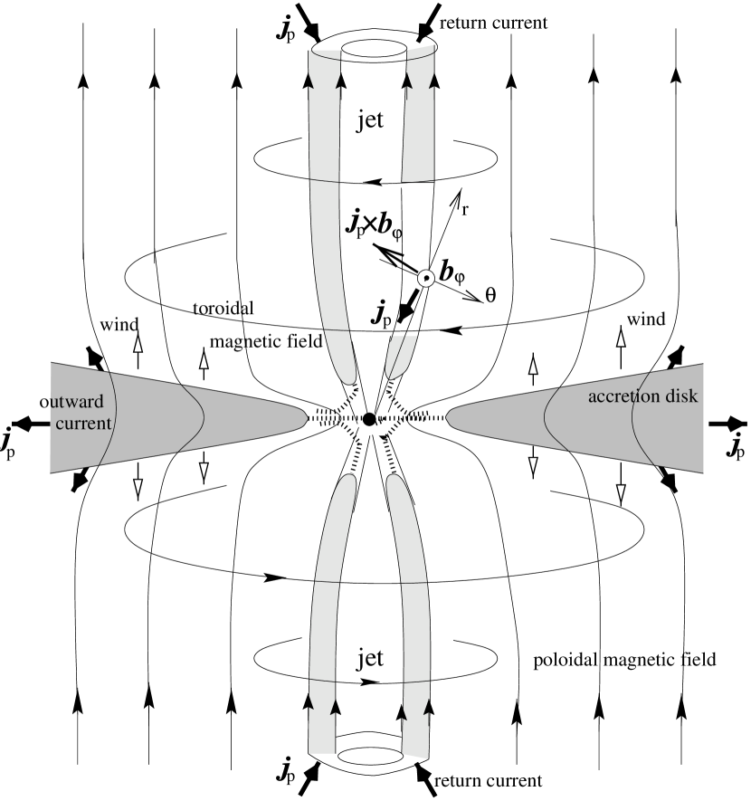
Figure 1: Conceptual drawing for illustration of the global configuration. The poloidal and toroidal components of the magnetic field lines are drawn with thin solid lines. The wind emanating from the disk surfaces and the poloidally circulating electric current are shown with white and black arrows, respectively. Also shown is the Lorentz force acting on the return current in the polar region, which has the components both for collimation and for radial acceleration of a jet. We distinguish jets from winds by their location and by the mechanisms for their generation.

We explain here the basic ideas and physical contents of the implicit wind model proposed in K01. A schematic drawing of the global configuration presumed in this model is given in Figure 1. An asymptotically uniform magnetic field is vertically penetrating the accretion disk and is twisted by the rotational motion of the plasma. Owing to the Maxwell stress of this twisted magnetic field, a certain fraction of the angular momentum of accreting plasma is carried away to infinity, and this fact ensures the plasma to gradually infall toward the central black hole. This infall sweeps the poloidal field lines toward the center, thus resulting in the amplification of the poloidal field in the disk. In this course, the gravitational energy of the infalling matter is converted into heat as a Joule dissipation of the current induced in the disk, because of a finite resistivity of the plasma.

In a stationary state, the deformation of magnetic field is determined by a balance between motional dragging and diffusive slippage of the field lines. Since the solution has been obtained under the assumption of large magnetic Reynolds number (i.e., $\Re^{2}(r)\gg 1$ in the disk, except the region close to its inner edge where $\Re\sim 1$), the field deformations are also large. In this sense the disk can be said as weakly resistive. The deformed part of the magnetic field and their sources (i.e., the electric currents in the disk) are obtained by solving a set of resistive MHD equations consistently with the fluid motion in the disk. Therefore, the presence of a large-scale seed field, which is assumed here to be uniform for simplicity, serves in our solution only to specify the boundary value at the disk’s outer edge. However, the presence of such a seed field whose origin can be attributed to some distant sources is essential in order not to conflict with the anti-dynamo theorem (e.g., Cowing 1981). The results also show that the deformation in the toroidal direction is larger than that in the poloidal direction (i.e., $b_{\varphi}/b_{\rm p}\sim\Re$, where $b$ denotes the deformed part of the magnetic field).

The vertical structure of the disk is maintained by a pressure balance between the magnetic pressure of the toroidal field, which is dominant outside the disk, and the gas pressure in the disk. Thus, the accreting plasma is magnetically confined in a geometrically thin disk. Reflecting this fact, the gas pressure and density in the disk become quantities of order $\Re^{2}$ (see, equations [49] and [58] in K01). In general, this balance is not a static balance in its strict sense, and there may be a vertical flow from the upper and lower surfaces of a disk. We call such outflows (or inflows depending on the case) winds, distinguished from jets that may be formed in the region within the inner edge of the accretion disk (also see below). A wind emanating from the accretion disk is not expected to form a relativistic jet after accelerated and collimated in the wind zone above the disk surfaces. Instead, the presence of winds may be important as a mechanism of supplying hot coronae around the disks.

Since the wind velocity obtained in K01 is much smaller than the rotational velocity (by a factor of order $\sim\Delta\Re^{-1}$, where $\Delta\ll 1$ is the half-opening angle of the disk) even at the disk surfaces, its inertial force can hardly affect the vertical force balance in the disk. However, the wind may be accelerated, by some mechanisms with which we do not concern in this paper, to a considerable speed after it has been injected from the accretion disk to the wind region outside the disk. Our main interest in the present paper (and in K01) is concentrated only on the launch of winds recognized within the disks. As for the final fate of the wind, we only expect that an upward wind proceeds to infinity because its total energy per unit mass (i.e., the Bernoulli sum in K01) is positive and hence the flow is unbound in the gravitational field.

It should be emphasized that, in the solution obtained in K01, the presence of such non-adiabaticities as discussed in the previous section exhibits itself solely in the radial profiles of the quantities such as density, pressure and magnetic field components (velocity components and temperature are not affected), but does not in the vertical profiles. Namely, if the radial dependences are less-steeper (i.e., $n>0$) than those in the critical case (i.e., $n=0$ as in the adiabatic solution of K00), an upward wind appears, and if they are steeper (i.e., $n<0$), a downward wind appears. The presence of a wind can be recognized also in the resulting radius-dependent mass accretion rate.

The rotational velocity is a certain fraction of the Kepler velocity (i.e., a reduced Keplerian rotation) because in this solution the radial pressure-gradient force, together with the centrifugal force, sustains the gravitational pull on the plasma. In contrast to the rotational velocity, the infall velocity is a small quantity of the order of $\Re^{-1}$ as far as the disk is weakly resistive (i.e., except for the region near the inner edge). As for the size of resistivity, we basically consider it to be specified by some anomalous transport processes caused by an MHD turbulence, a possible origin of which we have discussed in a separate paper (Kaburaki, Yamazaki & Okuyama 2002). Actually, however, we specify it implicitly in terms of the magnetic Reynolds number $\Re$ that is regarded as a free parameter, reflecting the rather poor current status of our understanding on the transport phenomena associated with turbulence.

The analytic solution obtained in K01 describes the physical quantities in the accretion disk (i.e., the solution is valid only in between the inner and outer edges of the disk) with also a decreasing accuracy toward the upper and lower surfaces of the disk. The latter part of this statement means that the solution contains a few inconsistencies of the order of $\tanh^{2}\eta$ in the vertical profiles of relevant quantities, where $\eta\equiv(\theta-\pi/2)/\Delta$ and $\theta$ is the colatitude. However, these inconsistencies can be safely neglected as far as the physics taking place near the disk midplane are concerned. We consider that the “main body” of an accretion disk occupying near the midplane, rather than its surface layers, plays an essential role in determining the wind launching, because this part contains the majority of plasma in the disk and hence energetically dominant over the surfaces layers. The vertical structure may probably be important in considering the origin of jets near the inner edge.

Further, the solution does not take care of the radiation losses. Nevertheless, since it has been confirmed retrospectively that the expected radiation flux from such a disk is negligibly small as far as the accretion rate is sufficiently smaller than the Eddington rate, the solution is self-consistent within this restriction.

If we extrapolate our physical understanding obtained within the disk even to the surrounding space, we are naturally led to the following picture of a galactic central engine. The engine is essentially a hydroelectric power station in which the ultimate energy source is the potential energy of the accreting plasma in the gravitational field. The accretion disk is a DC dynamo of an MHD type and drives mainly a poloidally circulating current system, which is the cause of the toroidal magnetic component added to the originally vertical field (i.e., the twisting of the field lines). In the configuration shown in figure 1, the radial current is driven outward in the accretion disk, and a part of the current closes its circuit through the near wind region while another part may close after circulating remote regions (probably reaching the boundary of a ‘cocoon’ enclosing hot winds). Anyway, these return currents concentrate within the polar regions in the upper and lower hemispheres, and finally return to the inner edge of the disk.

A bipolar jet may be formed from the plasma in this polar current regions, because the Lorentz force due to the toroidal field always has both of the necessary components for collimation and for radial acceleration, as shown in the figure. The often suggested universality of the association of an accretion disk and a bipolar jet is thus understood naturally in terms of one physical entity, the poloidally circulating current system. It is very likely that only a small fraction of the infalling matter input in the disk can actually fall onto the central black hole, with the remaining part expelled as a bipolar jet and a wind from disk surfaces.

In addition to the poloidal current system discussed above, there appears a toroidal current in the disk, which is the cause of the squeezed poloidal field lines. The toroidal current is maintained against the resistive dissipation by the electromotive force that results from an integration of the motional field along a toroidal ring. It may be worth noting here that this important possibility cannot help being dropped from the beginning in the ideal-MHD treatments. This is because, in that approximation, the motional field is exactly balanced by the electric field (i.e., $\mbox{\boldmath$E$}+(1/c)\mbox{\boldmath$v$}\times\mbox{\boldmath$B$}=0$), and hence the toroidal component of the motional field, which can be non-irrotational in general, is forced to vanish in a stationary, axisymmetric configuration according to vanishing toroidal electric field (i.e., $E_{\varphi}=0$; a more general discussion of the limitations of the ideal-MHD approximation can be seen in Kaburaki 1998).

3 BASIC EQUATIONS AND SIMPLIFYING ASSUMPTIONS

For the purpose of the present paper, we first modify the set of resistive-MHD equations to include the viscous force in the equation of motion:

$$\frac{D\mbox{\boldmath$v$}}{Dt}=-\frac{1}{\rho}\ \mbox{\boldmath$\nabla$}p-\frac{1}{4\pi\rho}\ [\mbox{\boldmath$B$}\times(\mbox{\boldmath$\nabla$}\times\mbox{\boldmath$B$})]+\mbox{\boldmath$g$}+\frac{\mbox{\boldmath$f$}}{\rho},$$ (1)

$$\frac{\partial\mbox{\boldmath$B$}}{\partial t}=\mbox{\boldmath$\nabla$}\times({\bf v}\times\mbox{\boldmath$B$})+\frac{c^{2}}{4\pi\sigma}\ \triangle\mbox{\boldmath$B$},\qquad(\sigma=\mbox{const.})$$ (2)

$$\frac{\partial\rho}{\partial t}+\mbox{\boldmath$\nabla$}\cdot(\rho\mbox{\boldmath$v$})=0,$$ (3)

$$\mbox{\boldmath$\nabla$}\cdot\mbox{\boldmath$B$}=0,$$ (4)

where

$$\frac{D\mbox{\boldmath$v$}}{Dt} \equiv \frac{\partial\mbox{\boldmath$v$}}{\partial t}+(\mbox{\boldmath$v$}\cdot\mbox{\boldmath$\nabla$})\mbox{\boldmath$v$}$$ (5)

$$= \frac{\partial\mbox{\boldmath$v$}}{\partial t}-\mbox{\boldmath$v$}\times[\mbox{\boldmath$\nabla$}\times\mbox{\boldmath$v$}]+\frac{1}{2}\ \mbox{\boldmath$\nabla$}v^{2},$$

$$f = \frac{4}{3}\ \mbox{\boldmath$\nabla$}(\rho\nu\mbox{\boldmath$\nabla$}\cdot\mbox{\boldmath$v$})-\mbox{\boldmath$\nabla$}\times[\mbox{\boldmath$\nabla$}\times(\rho\nu\mbox{\boldmath$v$})]+\mbox{\boldmath$\nabla$}[\mbox{\boldmath$v$}\cdot\mbox{\boldmath$\nabla$}(\rho\nu)]$$ (6)

$$+ \mbox{\boldmath$\nabla$}(\rho\nu)\times[\mbox{\boldmath$\nabla$}\times\mbox{\boldmath$v$}]-(\mbox{\boldmath$\nabla$}\cdot\mbox{\boldmath$v$})\ \mbox{\boldmath$\nabla$}(\rho\nu)-[\triangle(\rho\nu)]\mbox{\boldmath$v$}.$$

As usual, $v$, $\rho$ and $p$ denote velocity, density and pressure, respectively, of a fluid, and $B$ and $\sigma$, magnetic field and electric conductivity. The viscous force $f$ is expressed in terms of the kinematic viscosity $\nu$ only, because of Stokes’s relation.

In the above set of equations, the number of unknowns is formally 8: i.e., $v$, $b$, $p$, $\rho$. On the other hand, the number of independent equations is 7, owing to a degeneracy in Maxwell’s equations (see K00). The lacking equation is that of energy transport, which may in general be hopelessly complicated to be treated analytically. Therefore, it is often replaced by the assumption of polytrope, for simplicity. Since, however, there is no justification for the validity of the polytropic relation except for the special cases of adiabatic and isothermal processes, we rather let the set of equations open and discuss the energy balance after an explicit solution has been obtained.

In addition to the above 8 unknowns, actually we do not know how to specify the realistic sizes of viscosity $\nu$ and electric conductivity $\sigma$ from some fundamental theories. Namely, substantial number of unknowns is 10 instead of 8. Therefore, we need three more equations or constraints in order to select a definite IRAF solution among other possible types of solutions.

Once such a solution has been obtained, we can calculate other quantities of our interest from the following subsidiary equations. The electric field $E$, current density $j$ and charge density $q$ are, respectively, calculated from

$$E = \frac{\mbox{\boldmath$j$}}{\sigma}-\frac{1}{c}\ \mbox{\boldmath$v$}\ \times\mbox{\boldmath$B$},$$

$$j = \frac{1}{4\pi}\ \mbox{\boldmath$\nabla$}\times\mbox{\boldmath$B$},\quad q=\frac{1}{4\pi}\ \mbox{\boldmath$\nabla$}\cdot\mbox{\boldmath$E$}.$$ (7)

Temperature $T$, which is assumed to be common to electrons and ions under the expectation of a fairly turbulent plasma state, is given by the ideal gas law,

$$T=\frac{\bar{\mu}}{R}\ \frac{p}{\rho},$$ (8)

neglecting the radiation pressure ($\bar{\mu}$ is the mean molecular weight and $R$ is the gas constant).

According to the recipe of K00 and K01, we adopt spherical polar coordinates ($r$, $\theta$, $\varphi$) and simplify the above set of equations under the following assumptions. Namely, the flow is (i) stationary ($\partial/\partial t=0$) and (ii) axisymmetric ($\partial/\partial{\varphi}=0$), and the disk is (iii) geometrically thin, (iv) weakly viscous and weakly resistive, and we further admit (v) the dominance of the disk midplane.

The third assumption means that $\Delta\ll 1$, where $\Delta$ is the half-opening angle of the disk and is assumed to be constant. As stated in §2, the presence of the magnetic force guarantees the realization of such a thin disk, even in a hot IRAF situation (without this magnetic force the disk becomes geometrically thick; see, e.g., Kato, Fukue & Mineshige 1998). Reflecting this localized structure, we have introduced a normalized angular variable $\eta=(\theta-\pi/2)/\Delta$. Then, it becomes clear that a differentiation with respect to $\theta$ gives rise to a large quantity of order $\Delta^{-1}$ (i.e., $\partial/\partial\theta=\Delta^{-1}\partial/\partial\eta$). We can also safely assume in the disk that $\sin\theta\simeq 1$ and $\cos\theta\simeq 0$.

The statement (iv) implies that the “representative” values of the (viscous) Reynolds number $\Re_{\rm v}$ and the magnetic Reynolds number $\Re_{\rm m}$, whose precise definitions will be introduced later, are both large. We further assume that they are of the same order of magnitude so that $\Re^{2}_{\rm v}\sim\Re^{2}_{\rm m}\equiv\Re^{2}\gg 1$ in the disk (near the inner edge $r_{\rm in}$, however, $\Re\sim\Re_{\rm m}\sim 1$). This is because we are mainly interested in such a situation in the present paper, though in general there may be other possibilities. Namely, our present purpose is to examine whether the inclusion of a viscosity into otherwise-adiabatic accretion flow realized under the dominance of an ordered magnetic field can actually be altered to a non-adiabatic flow that can drive upward winds, or not.

The assumption (v) states our policy in considering the wind launching. Since the majority of matter is concentrated around the midplane of an accretion disk, it is natural to expect that the physical properties of the flow should be controlled primarily by this main body of the disk. Therefore, we may seek an approximate solution that is accurate near the midplane even if making a sacrifice of the accuracy near the upper and lower surfaces of the disk. According to this spirit, we ignore the quantities that are proportional to $\tanh^{2}\eta$ (except in the equation of vertical force balance where the vertical structure is essential), since $\tanh^{2}\eta\ll 1$, $\mbox{sech}^{2}\eta$ near the midplane. However, we do not intend to exclude the possibilities in which the forces that are important only near the disk surfaces can be essential in a different set up of the problems or in determining the subsequent acceleration of a wind. Our interest here is concentrated only on the initial indication of the wind launching. The important point is that there is indeed a meaningful solution by which we can discuss the physics of wind launching, within our restriction of the problems.

4 APPROXIMATE COMPONENT EQUATIONS

The method of obtaining the set of component expressions of resistive MHD equations simplified under the assumptions (i) through (v) is the same as described in K01. First we pick up only the leading order terms in $\Delta$ in each component equation, by regarding all quantities except $b_{\theta}$ and $v_{\theta}$ (which are of the order of $\Delta$ as specified by equations [14] and [15] below) are of order unity with respect to $\Delta$. Then further terms are dropped by the assumptions (iv) and (v). The only difference from the previous case may appear from the newly included term of viscous force in the equation of motion.

We cite below the set of simplified equations in the present case. It contains all terms that appeared in K01, and in addition, all of the contributions from the newly included viscous term (which can be identified easily by the presence of $\nu$) within the approximation to the leading order in $\Delta$.

1. Equation of motion:
   $r$-component,

   $$\frac{1}{\rho}\ \frac{\partial p}{\partial r}-\frac{GM}{r^{2}}-\frac{v_{\varphi}^{2}}{r}=\frac{1}{\rho r^{2}\Delta^{2}}\ \frac{\partial}{\partial\eta}\left(\rho\nu\frac{\partial v_{r}}{\partial\eta}\right)$$ (9)

   $\theta$-component,

   $$\frac{\partial p}{\partial\eta}+\frac{1}{8\pi}\ \frac{\partial b_{\varphi}^{2}}{\partial\eta}=0$$ (10)

   $\varphi$-component,

   $$\frac{v_{r}}{r}\frac{\partial}{\partial r}(rv_{\varphi})=\frac{b_{\theta}}{4\pi\rho r\Delta}\ \frac{\partial b_{\varphi}}{\partial\eta}$$ (11)

   $$+\frac{1}{\rho}\left[\frac{\partial}{\partial r}\left\{\rho\nu r\frac{\partial}{\partial r}\left(\frac{v_{\varphi}}{r}\right)\right\}+3\rho\nu\frac{\partial}{\partial r}\left(\frac{v_{\varphi}}{r}\right)\right]$$

2. Induction equation:
   poloidal component,

   $$\frac{v_{r}b_{\theta}}{c}=-\frac{c}{4\pi\sigma\Delta}\ \frac{1}{r}\frac{\partial b_{r}}{\partial\eta}$$ (12)

   $\varphi$-component,

   $$r^{2}b_{r}\frac{\partial}{\partial r}\left(\frac{v_{\varphi}}{r}\right)-\frac{\partial}{\partial r}(rv_{r}b_{\varphi})+\frac{c^{2}}{4\pi\sigma\Delta^{2}r}\ \frac{\partial^{2}b_{\varphi}}{\partial\eta^{2}}=0$$ (13)

3. Mass conservation,

   $$\frac{1}{r^{2}}\ \frac{\partial}{\partial r}(r^{2}\rho v_{r})+\frac{1}{\Delta r}\ \frac{\partial}{\partial\eta}(\rho v_{\theta})=0$$ (14)

4. Magnetic flux conservation,

   $$\frac{1}{r^{2}}\ \frac{\partial}{\partial r}(r^{2}b_{r})+\frac{1}{\Delta r}\ \frac{\partial b_{\theta}}{\partial\eta}=0$$ (15)

In the $r$-component of the equation of motion, the term on the right-hand side is a contribution from the viscous force. From its outlook, it may appear as a term of order $\Delta^{-2}$. However, one should be careful in evaluating the actual order of magnitude of this term because it contains the coefficient of viscosity $\nu$, the size of which is difficult to specify from a fundamental theory. At any rate, the representative size of this term can be written as $\sim\nu v_{r}/\Delta^{2}L^{2}$ while that of the gravity is $\sim v_{\rm K}^{2}/L$, where $L$ is a representative length-scale and $v_{\rm K}$ is the Kepler velocity. Recalling that $v_{r}\sim v_{\rm K}/\Re_{\rm m}$ (K00, K01), we can evaluate their ratio as $(\Delta^{2}\Re_{\rm v}\Re_{\rm m})^{-1}\sim(\Delta\Re)^{-2}$, where we have introduced $\Re_{\rm v}\equiv Lv_{\rm K}/\nu$ and used the assumption $\Re_{\rm v}\sim\Re_{\rm m}\equiv\Re$.

Thus, it turns out that the viscous term is much larger than the other terms (that are of order unity) as long as $(\Delta\Re)^{-2}\gg 1$, which will be confirmed later in §8 though $\Re$ may depend on $\Delta$ in general. Then, this term should vanish by itself since there is no other term that can balance it. Therefore, we have

$$\frac{\partial}{\partial\eta}\left(\rho\nu\frac{\partial v_{r}}{\partial\eta}\right)=0,$$ (16)

supplemented by

$$\frac{GM}{r^{2}}=\frac{v_{\varphi}^{2}}{r}-\frac{1}{\rho}\ \frac{\partial p}{\partial r},$$ (17)

from equation (9). We cannot drop the latter equation here as an equation of the next-leading order, because without it we cannot specify the rotational velocity. In this sense, we should regard rather that the former equation contains only a subsidiary information though it is a leading order equation (see also the discussion in the next section).

Another contribution from the viscous force appears in the $\varphi$-component of equation of motion (11). This equation describes the way in which the angular momentum is carried by the viscous stress as well as by the Maxwell stress. One can easily confirm that both terms on the right-hand side have the same order of magnitude, $v_{\rm K}^{2}/\Re L$ (where $\nu$ has been rewritten in terms of $\Re$), since $b_{\varphi}^{2}/(4\pi\rho)\sim v_{\rm K}^{2}$ as seen in the solution of K01.

The equation of vertical force balance (Eq. [10]) remains to be that of static balance in spite of the presence of a vertical flow, because the relevant inertial forces are negligibly small owing to its small speed even at the disk surfaces (i.e., $v_{\theta}\sim\Delta\Re^{-1}v_{\rm K}$).

5 SEPARATION OF VARIABLES

Here, we perform an approximate separation of variables for all the relevant quantities. The new factors we have to take care are the terms due to a finite viscosity: i.e., equation (16) and the second term on the right of equation (11). Since the former is a demand of the pure viscosity independent of the magnetic field, we first examine its implications. It is evident that equation (16) has a solution for $v_{r}$ that is independent of $\eta$, irrespective of the functional form of $\nu$. This means that a shear of $v_{r}$ in the vertical direction should vanish under the presence of even a weak viscosity. On the other hand, the purely hydromagnetic (i.e., inviscid) flows obtained in K00 and K01 have the vertical profile, $v_{r}\propto\mbox{sech}^{2}\eta$. These results are not compatible in a strict sense.

However, we are seeking only an approximate solution that is accurate only in the main body of an accretion disk, as expressed in the assumption (v). Within this approximation, the difference in the above two velocity profiles can be ignored, and we can regard that equation (16) has already been satisfied. Further, the new term in equation (11) does not cause any trouble if we assume that the viscosity has an angular profile of the form $\nu\propto\mbox{sech}^{2}\eta$.

Thus, we can follow the footsteps given in our previous papers and write

$$b_{r}(\xi,\eta)=\ \tilde{b}_{r}(\xi)\ \mbox{sech}^{2}\eta\tanh\eta,$$ (18)

$$b_{\theta}(\xi,\eta)=\ \tilde{b}_{\theta}(\xi)\ \mbox{sech}^{2}\eta,$$ (19)

$$b_{\varphi}(\xi,\eta)=-\tilde{b}_{\varphi}(\xi)\tanh\eta,$$ (20)

$$v_{r}(\xi,\eta)=-\tilde{v}_{r}(\xi)\ \mbox{sech}^{2}\eta,$$ (21)

$$v_{\theta}(\xi,\eta)=\tilde{v}_{\theta}(\xi)\tanh\eta,$$ (22)

$$v_{\varphi}(\xi,\eta)=\tilde{v}_{\varphi}(\xi),$$ (23)

$$p(\xi,\eta)=\ \tilde{p}(\xi)\ \mbox{sech}^{2}\eta,$$ (24)

$$\rho(\xi,\eta)=\ \tilde{\rho}(\xi)\ \mbox{sech}^{2}\eta,$$ (25)

$$\nu(\xi,\eta)=\ \tilde{\nu}(\xi)\ \mbox{sech}^{2}\eta,$$ (26)

$$T(\xi,\eta)=\tilde{T}(\xi),$$ (27)

$$j_{r}(\xi,\eta)=-\tilde{j}_{r}(\xi)\ \mbox{sech}^{2}\eta,$$ (28)

$$j_{\theta}(\xi,\eta)=\tilde{j}_{\theta}(\xi)\tanh\eta,$$ (29)

$$j_{\varphi}(\xi,\eta)=-\tilde{j}_{\varphi}(\xi)\ \mbox{sech}^{4}\eta,$$ (30)

$$E_{r}(\xi,\eta)=\tilde{E}_{r}(\xi)\ \mbox{sech}^{2}\eta,$$ (31)

$$E_{\theta}(\xi,\eta)=\tilde{E}_{\theta}(\xi)\ \mbox{sech}^{2}\eta\tanh\eta,$$ (32)

$$E_{\varphi}(\xi,\eta)=\tilde{E}_{\varphi}(\xi)\ \mbox{sech}^{4}\eta,$$ (33)

where the radial coordinate is normalized by a reference radius $r_{0}$ as $\xi=r/r_{0}$. In the problems of accretion in an ordered magnetic field, it is natural to choose the radius of disk’s outer edge, $r_{\rm out}$, as $r_{0}$. The sign of $\tilde{v}_{\theta}(\xi,\eta)$ is chosen in such a way that a positive $\tilde{v}_{\theta}$ corresponds to an upward wind (i.e., an outflow) from the disk surfaces.

Then, a set of ordinary differential equations for the radial parts follows from the set of simplified equations given in the previous section: that is

$$\frac{\tilde{v}_{\varphi}^{2}}{r}=\frac{1}{\tilde{\rho}}\ \frac{d\tilde{p}}{dr}+\frac{GM}{r^{2}},$$ (34)

$$\tilde{p}=\frac{\tilde{b}_{\varphi}^{2}}{8\pi},\quad(p+\frac{b_{\varphi}^{2}}{8\pi}=\tilde{p}),$$ (35)

$$\tilde{v}_{r}\frac{dl}{dr} = \frac{1}{4\pi\Delta}\ \frac{\tilde{b}_{\theta}\tilde{b}_{\varphi}}{\tilde{\rho}}$$ (36)

$$- \frac{r}{\tilde{\rho}}\left[\frac{d}{dr}\left(\tilde{\nu}\tilde{\rho}r\frac{d\Omega}{dr}\right)+3\tilde{\nu}\tilde{\rho}\frac{d\Omega}{dr}\right],$$

$$\tilde{v}_{r}\tilde{b}_{\theta}=\frac{c^{2}}{4\pi\sigma\Delta}\ \frac{\tilde{b}_{r}}{r},$$ (37)

$$\left(r^{2}\frac{d\Omega}{dr}\right)\tilde{b}_{r}-\frac{d}{dr}(r\tilde{v}_{r}\tilde{b}_{\varphi})+\frac{c^{2}}{2\pi\sigma\Delta^{2}}\ \frac{\tilde{b}_{\varphi}}{r}=0,$$ (38)

$$\frac{\tilde{v}_{\theta}}{\tilde{v}_{r}}=\Delta\left[r\frac{d}{dr}\ln(r^{2}\tilde{\rho}\tilde{v}_{r})\right],$$ (39)

$$\frac{\tilde{b}_{\theta}}{\tilde{b}_{r}}=\frac{\Delta}{2}\left[r\frac{d}{dr}\ln(r^{2}\tilde{b}_{r})\right],$$ (40)

where we have defined $l\equiv r\tilde{v}_{\varphi}$ and $\Omega\equiv\tilde{v}_{\varphi}/r$.

In addition to the above set, the subsidiary equations are reduced to

$$\tilde{T}=\frac{\bar{\mu}}{R}\ \frac{\tilde{p}}{\tilde{\rho}},$$ (41)

$$\tilde{j}_{r}=\frac{c}{4\pi\Delta}\ \frac{\tilde{b}_{\varphi}}{r},$$ (42)

$$\tilde{j}_{\theta}=\frac{c}{4\pi}\ \frac{1}{r}\frac{d}{dr}(r\tilde{b}_{\varphi}),$$ (43)

$$\tilde{j}_{\varphi}=\frac{c}{4\pi\Delta}\ \frac{\tilde{b}_{r}}{r},$$ (44)

$$\tilde{E}_{r}=-\frac{\Delta}{2}\ \frac{d}{dr}(r\tilde{E}_{\theta})=\frac{1}{c}\left(\tilde{v}_{\varphi}\tilde{b}_{\theta}-\frac{c^{2}}{4\pi\sigma\Delta}\ \frac{\tilde{b}_{\varphi}}{r}\right),$$ (45)

$$\tilde{E}_{\theta}=\frac{1}{c}\ (\tilde{v}_{r}\tilde{b}_{\varphi}-\tilde{v}_{\varphi}\tilde{b}_{r}),$$ (46)

$$\tilde{E}_{\varphi}=\frac{1}{c}\ \left(\tilde{v}_{r}\tilde{b}_{\theta}-\frac{c^{2}}{4\pi\sigma\Delta}\ \frac{\tilde{b}_{r}}{r}\right)=0,$$ (47)

where $\tilde{E}_{\varphi}$ is forced to vanish owing to the assumption (ii) and this is actually confirmed from equation (37).

6 SCALING CONDITIONS

In order to select the IRAF solution from other types of solutions to the set of ordinary differential equations obtained in the previous section, we introduce three additional constraints here. These are called the scaling conditions, because they specify the radial scaling of some quantities in the manner that the gravity requires. These constraints result in a simple power-law dependence for the radial part of each physical quantity, which is the characteristic feature of our wind solutions.

The first of them is the major condition in selecting the IRAF solution, which is characterized essentially by a virial-type temperature (note that the numerator is a quantity of $\sim T/r$):

$$\alpha \equiv -\frac{1}{\rho}\frac{\partial p}{\partial r}\biggm{/}\frac{GM}{r^{2}}$$ (48)

$$= -\frac{1}{\tilde{\rho}}\frac{d\tilde{p}}{dr}\biggm{/}\frac{GM}{r^{2}}={\rm const.}\ (<1).$$

Then, we obtain from equation (17) or (34) a reduced Keplerian rotation of the form

$$v_{\varphi}=\tilde{v}_{\varphi}=(1-\alpha)^{1/2}\ v_{\rm K}(r),$$ (49)

where $v_{\rm K}(r)\equiv(GM/r)^{1/2}$ is the Kepler velocity. It should be noted also that the assumption of constant $\Delta$ is consistent with the appearance of a virial-type temperature (see, the appendix of K00).

In a similar manner, the second condition requires that

$$\beta \equiv \frac{1}{b_{r}}\ \frac{\partial}{\partial r}(rv_{r}b_{\varphi})\biggm{/}r^{2}\frac{\partial}{\partial r}\left(\frac{v_{\varphi}}{r}\right)$$ (50)

$$= \frac{1}{\tilde{b}_{r}}\ \frac{d}{dr}(r\tilde{v}_{r}\tilde{b}_{\varphi})\biggm{/}r^{2}\ \frac{d\Omega}{dr}=\mbox{const.}\ (<1),$$

where $\Omega\equiv\tilde{v}_{\varphi}/r$ is also specified by the gravity through equation (49). Then, equation (13), or (38) reduces to

$$\tilde{b}_{r}=-\frac{c^{2}}{2\pi(1-\beta)\sigma\Delta^{2}}\left(r^{3}\frac{d\Omega}{dr}\right)^{-1}\tilde{b}_{\varphi}.$$ (51)

Substituting equation (49) for $\Omega$, we obtain

$$\frac{\tilde{b}_{\varphi}}{\tilde{b}_{r}}=\frac{3\pi(1-\beta)\Delta^{2}\sigma}{c^{2}}\ (1-\alpha)^{1/2}l_{\rm K}\equiv\Re_{\rm m}(r),$$ (52)

where $l_{\rm K}\equiv\sqrt{GMr}$. Since the right-hand side has a form of magnetic Reynolds number, we adopt this as a representative value of the magnetic Reynolds number that is characteristic to the present problem. With the aid of this definition of $\Re_{\rm m}$ in (52), we can always replace $\sigma$ in terms of $\Re_{0}\equiv\Re_{\rm m}(r_{0})$ by regarding the latter as a free parameter of the present model.

The third condition requires that the fraction of the viscous angular-momentum transport among the total transport is a constant:

$$\gamma \equiv \frac{1}{\rho}\left[\frac{\partial}{\partial r}\left\{\rho\nu r\frac{\partial}{\partial r}\left(\frac{v_{\varphi}}{r}\right)\right\}+3\rho\nu\frac{\partial}{\partial r}\left(\frac{v_{\varphi}}{r}\right)\right]\biggm{/}\frac{v_{r}}{r}\ \frac{\partial}{\partial r}(rv_{\varphi})$$ (53)

$$= -\frac{1}{\tilde{\rho}}\left[\frac{d}{dr}\left(\tilde{\nu}\tilde{\rho}r\frac{d\Omega}{dr}\right)+3\tilde{\nu}\tilde{\rho}\frac{d\Omega}{dr}\right]\biggm{/}\frac{\tilde{v}_{r}}{r}\ \frac{dl}{dr}=\mbox{const.}\ (<1).$$

As we shall see explicitly in the next section, this condition reduces to a phenomenological prescription of the viscosity $\tilde{\nu}(\xi)$ in terms of a free parameter $\gamma$. Combining the above condition (53) with equation (36), we obtain

$$(1-\gamma)\ \tilde{v}_{r}\frac{dl}{dr}=\frac{\tilde{b}_{\theta}\ \tilde{b}_{\varphi}}{4\pi\Delta\tilde{\rho}}.$$ (54)

7 VISCOUS-WIND SOLUTION

The IRAF-type solution that is selected under the above three scaling conditions will be called the viscous-wind solution. The procedure to obtain it is quite analogous to the case of K01, and rather straightforward. Namely, we start from the following form for the poloidal magnetic field,

$$\tilde{b}_{r}(\xi)=B_{0}\ \xi^{-(3/2-n)},$$ (55)

where the parameter $n$ describes the deviation from the adiabatic case ($n=0$) in which no wind appears (K00).

Substituting the above expression into equations (52) and (40), we obtain

$$\tilde{b}_{\varphi}(\xi) = \Re_{0}B_{0}\ \xi^{-(1-n)}$$ (56)

where

$$\Re_{0} = \frac{3\pi(1-\alpha)^{1/2}(1-\beta)\sigma\Delta^{2}}{c^{2}}\ l_{{\rm K}0},$$ (57)

and

$$\tilde{b}_{\theta}(\xi)=\frac{2n+1}{4}\ \Delta B_{0}\ \xi^{-(3/2-n)},$$ (58)

respectively. Then, it follows from equation (35) that

$$\tilde{p}(\xi)=\frac{\Re^{2}_{0}B_{0}^{2}}{8\pi}\ \xi^{-2(1-n)}.$$ (59)

The subscript 0 is referred to each quantity at $r_{0}$.

Using the expressions for $\tilde{b}_{r}$ and $\tilde{b}_{\theta}$, we obtain from equation (37)

$$\tilde{v}_{r}(\xi)=\frac{3(1-\alpha)^{1/2}(1-\beta)}{2n+1}\ \frac{v_{{\rm K}0}}{\Re_{0}}\ \xi^{-1},$$ (60)

and further from this result and equation (39),

$$\tilde{v}_{\theta}(\xi)=\frac{6(1-\alpha)^{1/2}(1-\beta)n}{2n+1}\ \frac{\Delta v_{{\rm K}0}}{\Re_{0}}\ \xi^{-1}.$$ (61)

The density is calculated from equation (54) as

$$\tilde{\rho}(\xi)=\frac{(2n+1)^{2}}{24\pi(1-\alpha)(1-\beta)(1-\gamma)}\ \frac{\Re^{2}_{0}B_{0}^{2}}{v_{{\rm K}0}^{2}}\ \xi^{-(1-2n)}$$ (62)

With the above temporal expressions for various quantities, we can determine first $\beta$ from the second scaling condition (50) and then $\alpha$ from the first scaling condition (48) as

$$\alpha = \frac{2(1-n)(1-\gamma)}{3-2(1-n)\gamma},$$ (63)

$$\beta = \frac{2}{3}(1-n),$$ (64)

Therefore, the above temporal expressions finally become

$$\Re(\xi)=\Re_{0}\ \xi^{1/2},\quad\Re_{0}=\sqrt{\frac{(2n+1)^{3}}{3-2(1-n)\gamma}}\ \frac{\pi\sigma\Delta^{2}l_{{\rm K}0}}{c^{2}}$$ (65)

$$\tilde{v}_{r}(\xi)=\sqrt{\frac{2n+1}{3-2(1-n)\gamma}}\ \frac{v_{{\rm K}0}}{\Re_{0}}\ \xi^{-1},$$ (66)

$$\tilde{v}_{\theta}(\xi)=2n\sqrt{\frac{2n+1}{3-2(1-n)\gamma}}\ \frac{\Delta v_{{\rm K}0}}{\Re_{0}}\ \xi^{-1},$$ (67)

$$\tilde{v}_{\varphi}(\xi)=\sqrt{\frac{2n+1}{3-2(1-n)\gamma}}\ v_{{\rm K}0}\ \xi^{-1/2},$$ (68)

$$\tilde{\rho}(\xi)=\frac{3-2(1-n)\gamma}{8\pi(1-\gamma)}\ \frac{\Re^{2}_{0}B_{0}^{2}}{v_{{\rm K}0}^{2}}\ \xi^{-(1-2n)},$$ (69)

and for the subsidiary equations,

$$\tilde{T}(\xi)=\frac{1-\gamma}{3-2(1-n)\gamma}\ \frac{\bar{\mu}v_{{\rm K}0}^{2}}{R}\ \xi^{-1},$$ (70)

$$\tilde{j}_{r}(\xi)=\left(\frac{c}{4\pi\Delta}\right)\frac{\Re_{0}B_{0}}{r_{0}}\ \xi^{-(2-n)},$$ (71)

$$\tilde{j}_{\theta}(\xi)=n\left(\frac{c}{4\pi}\right)\ \frac{\Re_{0}B_{0}}{r_{0}}\ \xi^{-(2-n)},$$ (72)

$$\tilde{j}_{\varphi}(\xi)=\left(\frac{c}{4\pi\Delta}\right)\ \frac{B_{0}}{r_{0}}\ \xi^{-(5/2-n)},$$ (73)

$$\tilde{E}_{r}(\xi)=\tilde{E}_{\theta}(\xi)=\tilde{E}_{\varphi}(\xi)=0.$$ (74)

The $r$-dependences of all relevant quantities are the same as in K01, and the parameter $\gamma$ appears only in their coefficients. Therefore, the allowed range for $n$ remains the same as before, i.e., $-1/4<n<1/2$. It is a conspicuous character of our wind solutions (irrespective of implicit or explicit type) that the radial part of each quantity are written in a simple power-law form, as a consequence of the scaling conditions. Since, however, the quantities depend generally on the two variables, $\xi$ and $\eta$, the solution is not of a self-similar type in which every quantity depends only on a definite combination of these variables.

Finally from the third scaling condition (53), we have

$$\tilde{\nu}(\xi)=\mbox{const.}\equiv\nu_{0},$$ (75)

and solving the resulting expression of $\gamma$ for $\nu_{0}$,

$$\nu_{0}=\frac{2\gamma}{3(4n+1)}\ \sqrt{\frac{2n+1}{3-2(1-n)\gamma}}\ v_{{\rm K}0}\ \frac{r_{0}}{\Re_{0}}.$$ (76)

Since $n$ is uniquely specified by $\gamma$ (see the next section), the latter relation serves as a phenomenological prescription of the viscosity in terms of a viscous parameter $\gamma$. This equation shows that $\Re_{\rm v}\equiv l_{{\rm K}0}/\nu_{0}\sim\Re_{0}$ as expected, since $\gamma$ and $n$ are the quantities of order unity. Here, we can see some analogy to the $\alpha$-prescription, $\nu=\alpha V_{\rm S}H$ (where $V_{\rm S}$ is the sound velocity and $H$ is the half-thickness of a disk; Shakura & Sunyaev 1973; Frank, King, & Raine 1992) since $V_{\rm S}\sim v_{\rm K}$ in our solution. It may be even closer to the $\beta$-prescription of Duschl, Strittmatter & Biermann (2000), $\nu=\beta v_{\varphi}r$ where $\beta$ is a parameter of order $\sim\Re_{\rm v}^{-1}$.

8 ENERGY BALANCE

In order to discuss in detail the energy budget in an accretion disk, we have to derive some more relations describing global aspects of the present solution. From the definition of the disk’s inner edge (i.e., $\Re(\xi_{\rm in})=1$) and equation (65), we obtain

$$\xi_{\rm in}=\Re_{0}^{-2},$$ (77)

and the condition $r_{\rm in}\ll r_{\rm out}$ guarantees that $\Re_{0}^{-2}\ll 1$. The conservation of magnetic flux applied to the field penetrating the disk,

$$\pi r_{\rm in}^{2}\ \tilde{b}_{r}(r_{\rm in})=\int_{r_{\rm in}}^{r_{\rm out}}\tilde{b}_{\theta}\ 2\pi r\ dr,$$ (78)

yields the relation

$$\Delta=\frac{\xi_{\rm in}^{n+1/2}}{1-\xi_{\rm in}^{n+1/2}}\simeq\xi_{\rm in}^{n+1/2}=\Re_{0}^{-(2n+1)}.$$ (79)

In the above equation, the approximate expression holds because $\xi_{\rm in}^{n+1/2}\ll 1$ when $-1/4<n<1/2$. We can show also that $(\Delta\Re_{0})^{-2}=\Re_{0}^{4n}\gg 1$ for $n>0$, except for $n$ very close to 0. Even in this exceptional case of vanishing $n$ (then we have $(\Delta\Re_{0})^{-2}\sim 1$), equation (9) can be still satisfied if we simply maintain the requirements, equations (16) and (17), obtained in the case of non-vanishing $n$.

Owing to the presence of vertical flows, the mass accretion rate becomes a function of radius like

$$\dot{M}(\xi)=-\int_{-\infty}^{\infty}2\pi\rho v_{r}r^{2}\Delta\ d\eta=\dot{M}_{0}\ \xi^{2n},$$ (80)

where

$$\dot{M}_{0}=\frac{\sqrt{(2n+1)[3-2(1-n)\gamma]}}{3(1-\gamma)}\ \frac{B_{0}^{\ 2}r_{0}^{2}}{\Re_{0}^{2n}v_{{\rm K}0}}.$$ (81)

The latter equation can be used to express $r_{0}$ in terms of $B_{0}$ and $\dot{M}_{0}$, or $B_{0}$ in terms of $\dot{M}_{0}$ and $r_{0}$. We can introduce also the mass-ejection rate due to a part of the wind within an arbitrary radius $r$, by

$$\dot{M}_{\rm w}(\xi)\equiv\dot{M}(\xi)-\dot{M}_{\rm in}=\dot{M}_{0}\ (\xi^{2n}-\xi_{\rm in}^{2n}).$$ (82)

It should be noted that this expression does not include the mass loss associated with a possible jet expected to be within the disk’s inner edge.

Since we have not used the energy equation in obtaining the viscous-wind solution, it is not satisfied yet. Rather, the requirement of energy balance determines the relation between $n$ and $\gamma$ as confirmed below. The Joule heating rate is calculated as

$$q_{\rm J}^{+}(\xi,\eta)=\frac{\mbox{\boldmath$j$}^{2}}{\sigma}\sim\frac{j_{r}^{2}}{\sigma}$$ (83)

$$=\frac{3(1-\gamma)(2n+1)}{16\pi[3-2(1-n)\gamma]}\ \Re_{0}^{2n+1}\ \frac{GM\dot{M}_{0}}{r_{0}^{4}}\ \xi^{-2(2-n)}\mbox{sech}^{4}\eta,$$

where $c^{2}/\sigma\Delta^{2}$ and $B_{0}^{2}$ have been eliminated by the aid of equations (65) and (81). The viscous heating rate is given by

$$q_{\rm vis}^{+}(\xi,\eta)=\nu\rho\left(\xi\frac{d\Omega}{d\xi}\right)^{2}$$ (84)

$$=\frac{9\gamma(2n+1)}{16\pi(4n+1)[3-2(1-n)\gamma]}\ \Re_{0}^{2n+1}\ \frac{GM\dot{M}_{0}}{r_{0}^{4}}\ \xi^{-2(2-n)}\mbox{sech}^{4}\eta,$$

where the expression for $\nu_{0}$ (eq. [76]) has been used. The advection cooling, on the other hand, is

$$q_{\rm adv}^{-}(\xi,\eta)\equiv\mbox{\boldmath$\nabla$}\cdot(h\rho\mbox{\boldmath$v$})-(\mbox{\boldmath$v$}\cdot\mbox{\boldmath$\nabla$})\ p$$ (85)

$$=\frac{1}{r^{2}}\frac{\partial}{\partial r}(r^{2}h\rho v_{r})+\frac{1}{r\Delta}\frac{\partial}{\partial\eta}(h\rho v_{\theta})-v_{r}\frac{\partial p}{\partial r}-\frac{v_{\theta}}{r\Delta}\frac{\partial p}{\partial\eta}$$

$$=\frac{3(1-\gamma)(4n+1)}{16\pi[3-2(1-n)\gamma]}\ \Re_{0}^{2n+1}\ \frac{GM\dot{M}_{0}}{r_{0}^{4}}\ \xi^{-2(2-n)}\ \mbox{sech}^{4}\eta,$$

where the last term in the second line has been dropped on account of the assumption (v).

Since the radial dependences of the viscous-wind solution are identical with that of the implicit-wind solution (K01), the optical depth, for the electron scattering, in the vertical direction of the accretion disk is a quantity of similar orders of magnitude to the value given as equation (9) in Yamazaki, Kaburaki & Kino (2002). There, one can see that the radiative cooling may be negligible as far as the mass accretion rate is sufficiently small compared with the Eddington rate. This fact has also been confirmed by the explicit calculations of radiation losses based on the analytic models of K00 and K01, respectively, in Kino, Kaburaki & Yamazaki (200) and in Yamazaki, Kaburaki & Kino (2002). These works show that only the synchrotron and associated inverse Compton losses in the region very close to the inner edge can be non-negligible (compared with the advection cooling), because of a relativistic temperature there.

Then, the local energy balance in a stationary state should be

$$q^{+}_{\rm J}+q^{+}_{\rm vis}=q^{-}_{\rm adv},$$ (86)

except in the region very close to the inner edge. Substituting the above $q$’s into equation (86), we obtain

$$f(n)\equiv 8(1-\gamma)n^{2}+2(1-4\gamma)n-3\gamma=0.$$ (87)

The quadratic function of $n$ expresses a downwardly convex parabola for a given $\gamma$ in the range $0\leq\gamma<1$. In the inviscid limit ($\gamma=0$), it has two solutions, $n=0$ and $n=-1/4$. The former corresponds to the completely advective flow of K00, and the latter, to the isentropic flows where $q_{\rm adv}^{-}=0$. However, the latter case should be removed from our consideration because $q_{\rm viss}^{+}$ becomes negative then.

For a general viscous fluid with $\gamma>0$, we have $f(0)=-3\gamma<0$ and this means that one root of equation (87) is always positive while the other root is always negative. Further, the fact that $f(-1/4)=-(3/2)\gamma<0$ means that the negative root is smaller than $-1/4$. In order for the positive root remains within the range $n<1/2$, one should require that $f(1/2)=3(1-3\gamma)>0$. To summarize, we have a root of equation (87) within the range $0\leq n<1/2$ for a given viscosity parameter in the range $0\leq\gamma<1/3$, and the root is

$$n=\frac{4\gamma-1+\sqrt{-8\gamma^{2}+16\gamma+1}}{8(1-\gamma)}.$$ (88)

Therefore, a non-zero viscosity always drive an upward wind ($n>0$; see figure 2).

Hitherto, we have regarded the appearance of a positive $v_{\theta}$ as the launching of a wind, in spite of the fact that our solution is valid only within the main body of an accretion disk and we do not discuss the subsequent acceleration or deceleration. This is because we can guess the final fate of the vertical flow from the sign of the Bernoulli sum that is defined as the total energy per unit mass of a fluid element:

$$B_{\rm e}(\xi,\eta)\equiv\frac{1}{2}v^{2}-\frac{GM}{r}+h,$$ (89)

where the terms on the right-hand side are the kinetic, gravitational and thermal energies ($h$ is the specific enthalpy), respectively. Since we adopt the ideal gas law (8), we have $h=(5/2)p/\rho$ irrespective of the assumption of polytrope. If this sum is negative the fluid element is bound in the gravitational field, but if it is positive the fluid is unbound and can reach infinity.

The energy of the magnetic field should not be included in the above definition, because the flow does not carry around the field lines (in contrast to the ideal-MHD case) in a stationary state. In a stationary accretion process, the field acts only as a catalyst to convert gravitational energy into other forms (e.g., thermal energy). Especially in our wind solutions, the magnetic field does not even transport energy in terms of the MHD Poynting flux since the electric field vanishes there. This means that energy exchange among fluid elements through the Poynting flux does not play any role in our wind models, and hence the whole energy associated with the magnetic extraction of angular momentum is released locally within the disk as a Joule dissipation. In terms of the “angular velocity” of the magnetic field, $\Omega_{\rm F}$, this corresponds to the case of $\Omega_{\rm F}=0$, and in terms of the circuit theory, this does to the case of no external load.

Now, the remaining task in the present section is to confirm that the wind identified by a positive $n$ in the range $0<n<1/2$ actually have a positive Bernoulli sum. Since the kinetic energy is dominated by its rotational part, the sum is calculated to be

$$B_{\rm e}(\xi,\eta)\simeq\frac{1}{2}v_{\varphi}^{\ 2}-\frac{GM}{r}+h=\frac{2n-(4n+1)\gamma}{2[3-2(1-n)\gamma]}\ v_{{\rm K}0}^{\ 2}\ \xi^{-1},$$ (90)

which is independent of $\eta$. If we rewrite the coefficient there as $\gamma(2n+1)(1-2n)/(4n+1)[3-2(1-n)\gamma]$ by the aid of equation (87), it becomes evident that the expression on the rightmost side of the above equation is always positive for $0<n<1/2$ and hence for $0<\gamma<1/3$ (see also figure 2). Although $B_{\rm e}$ becomes zero in the limit of $\gamma=1/3$, it corresponds to the unrealistic limit of $n=1/2$ in which the density becomes independent of the radius. This limit has therefore been excluded from our consideration from the beginning.

In general accretion flows, the Bernoulli sum is not conserved along stream lines. When the flow is adiabatic, however, it is conserved. This is evident from the following consideration. Namely, in the course of gradual infall process, a part of the gravitational energy of a fluid element goes to its rotational energy and the rest is released as thermal energy. If there is no mechanism of energy exchange through the boundary of the fluid element (i.e., the flow is adiabatic), the liberated energy remains within the element. In this case the Bernoulli sum remains the same along each stream line, because the result of the infall is a decrease in the gravitational energy that is exactly compensated by the increases in the kinetic and thermal energies.

Therefore, if the accreting matter falls from infinity with marginally bound condition (i.e., with $B_{\rm e}=0$), it will remain so unless some mechanism of energy transport intervenes. In many cases, the radiative cooling carries away a considerable part of energy from the fluid and it becomes bound (i.e.,$B_{\rm e}<0$). In IRAFs, however, this cannot be expected and hence other types of energy exchange such as convection, conduction or viscous transport controls the fate of the accretion flow.

It has turned out in this section that the viscosity always acts as a net source of heating for the disk and drives upward wind from its surfaces. If we extrapolate this result to the region within the inner edge of the accretion disk, we can say that there should be an infalling part of the flow with negative Bernoulli sum, which is a direct consequence of the outward transport of energy by the viscosity. In other words, a part of the accretion flow in an IRAF state can really fall onto the central object only when the flow can expel the other part as wind or jet (a basic idea of this point can be seen in Blandford 1999).

9 SUMMARY AND CONCLUSION

In order to construct an explicit example of the disk wind model in which a non-adiabatic exchange of energy drives the wind, we have included the viscosity into the otherwise adiabatic model (K00) of accretion flows in an ordered magnetic field. Under a plausible set of simplifying assumptions, we have derived an analytic solution to the set of resistive MHD equations among which the equation of motion contains the viscous force term. It describes an inefficiently-radiating accretion flow (IRAF), in which the angular momentum of the accreting plasma is extracted simultaneously by the Maxwell stress of the twisted magnetic field and by the viscous torque. Associated with the latter process, energy is transported outwardly and the resultant heating of the disk becomes the cause of an upward wind.

From the condition of energy balance, the wind parameter $n$ is uniquely specified in terms of our viscosity parameter $\gamma$. It has turned out that, for the allowed range of $\gamma$, $n$ is always positive indicating that the viscosity always drives an upward wind. Although we can only infer the final fate of the wind from the sign of the Bernoulli sum, it indicates that the wind with positive $n$ within the allowed range of the model will indeed reach the infinity. We can also speculate that, owing to this outward energy transport by the viscosity, at least, a part of the flow within the disk’s inner edge becomes able to fall onto the central object with negative Bernoulli sum.

It is very subtle to specify the type of wind launching as centrifugal or thermal. Although the addition of thermal energy to a disk is essential as the cause of a wind launching, the force due to vertical pressure gradient is balanced by that of the magnetic pressure gradient, within our approximation. Similarly, the horizontal component of the gravitational force is balanced by the centrifugal force plus the radial pressure gradient, within the same approximation. However, it should be noted that the wind velocity is proportional to $n$ and $n$ increases with decreasing $\alpha$ (see figure 2). Since the rotational velocity increases with decreasing $\alpha$, this means that the upward wind appears only when the disk rotates faster than a critical value. Thus, we prefer the interpretation of centrifugally driven wind.

If we may assume that the wind region extending above and below the surfaces of an accretion disk is well described by the ideal-MHD, we can roughly estimate the terminal velocity of a wind. Since, then, the Bernoulli sum is conserved along the magnetic surface on which the flow travels, we have

$$v_{\infty}\sim\sqrt{\frac{2n-(4n+1)\gamma}{3-2(1-n)\gamma}}\ v_{\rm K}(r),$$ (91)

where $r$ denotes the footpoint radius of the magnetic surface. In deriving the above expression, we have assumed that both rotational and thermal energy decrease to zero at infinity. The coefficient $\sqrt{2\bar{B}_{\rm e}}$ is less than about 0.25 (see figure 2).

Figure 2: Behavior of the parameters, $\alpha$, $\beta$ and $n$, and of the normalized Bernoulli sum, $\bar{B}_{\rm e}$, all as functions of the viscous parameter $\gamma$. The definition of the latter is $\bar{B}_{\rm e}\equiv B_{\rm e}/v_{{\rm K}0}\xi^{-1}$, and it represents the coefficient in equation (90). The upper most value of $\gamma$ is 1/3.

References

- (1)
- (2) Abramowicz, M. A., Chen, X., Kato, S., Lasota, J.-P., & Regev, O. 1995, ApJ, 438, L37
- (3) Blandford, R. D. 1999, in Galaxy Dynamics, eds. D. Merritt, J. A. Sellwood & M. Valluri (ASP Conf. Ser. vol. 182, Astron. Soc. Pac., San Francisco), 87
- (4) Blandford, R. D., & Begelman, M. C. 1999, MNRAS, 303, L1
- (5) Blandford, R. D., & Payne, D. G. 1982, MNRAS, 199, 883
- (6) Casse, F., & Ferreira, J. 2000, A&A, 361, 1178
- (7) Chakrabarti, S. K. 1998, in Black Holes: Theory and Observation, ed. F. W. Hehl, C. Kiefer & R. J. K. Metzler (Springer), 80
- (8) Chen, X., Abramowicz, M. A., Lasota, J.-P., Narayan, R., & Yi 1995, ApJ, 443, L61
- (9) Cowling, T. G. 1981, ARA&A, 19, 115
- (10) Duschl, W. J., Strittmatter, P. A., & Biermann, P. L. 2000, A&A, 357, 1132
- (11) Ferreira, J. & Pelletier, G. 1993, A&A, 295, 807
- (12) Frank, J., King, A., & Raine, D. 1992, Accretion Power in Astrophysics (Cambridge: Cambridge Univ. Press)
- (13) Ichimaru, S. 1977, ApJ, 214, 840
- (14) Kaburaki, O. 1998, in Neutron Stars and Pulsars: Thirty Years after the Discovery, ed. N. Shibazaki et al. (Tokyo: Universal Academy Press), 515
- (15) Kaburaki, O. 2000, ApJ, 531, 210 (K00)
- (16) Kaburaki, O. 2001, ApJ, 563, 505 (K01)
- (17) Kaburaki, O., Yamazaki, N., & Okuyama, Y. 2002, NewA. 7, 283
- (18) Kato, S., Fukue, J. & Mineshige, S. 1998, Black-Hole Accretion Disks (Kyoto: Kyoto Univ. Press)
- (19) Kino, M., Kaburaki, O. & Yamazaki, N. 2000, ApJ, 536, 788
- (20) Lasota, J.-P. 1999, Phys. Rep. 311, 247
- (21) Lubow, S. H., Papaloizou, J. C. & Pringle, J. E. 1994, MNRAS, 268, 1010
- (22) Nakamura, K. E. 1998, PASJ, 50, L11
- (23) Narayan, R., & Yi, I. 1994, ApJ, 428, L13
- (24) Narayan, R., & Yi, I. 1995, ApJ, 444, 231
- (25) Narayan, R., Igumenshchev, I. V., & Abramowicz, M. A. 2000, ApJ, 539, 798
- (26) Narayan, R., Mahadevan, R., & Quataert, E. 1998, in Theory of Black Hole Accretion Disks, ed. M. A. Abramowicz, G. Bjornsson, & J. E. Pringle (Cambridge: Cambridge University Press), 148
- (27) Quataert, E., & Gruzinov, A. 2000, ApJ, 539, 809
- (28) Shakura, N. I., & Sunyaev, R. A. 1973, A&A, 24, 337
- (29) Wardle, M. I., & Königl, A. 1993, ApJ, 410, 218
- (30) Yamazaki N., Kaburaki, O. & Kino, M. 2002, MNRAS, 337, 1357
- (31)