Modeling of iron K lines: radiative and Auger decay data for Fe ii–Fe ix

A detailed analysis of the radiative and Auger de-excitation channels of K-shell vacancy states in Fe ii–Fe ix has been carried out. Level energies, wavelengths, $A$-values, Auger rates and fluorescence yields have been calculated for the lowest fine-structure levels populated by photoionization of the ground state of the parent ion. Different branching ratios, namely K$\alpha_{2}$/K$\alpha_{1}$, K$\beta$/K$\alpha$, KLM/KLL, KMM/KLL, and the total K-shell fluorescence yields, $\omega_{K}$, obtained in the present work have been compared with other theoretical data and solid-state measurements, finding good general agreement with the latter. The K$\alpha_{2}$/K$\alpha_{1}$ ratio is found to be sensitive to the excitation mechanism. From these comparisons it has been possible to estimate an accuracy of $\sim$10% for the present transition probabilities.

1 Introduction

The iron K lines appear in a relatively unconfused spectral region and have a high diagnostic potential. The study of these lines has been encouraged by the quality spectra emerging from Chandra and by the higher resolution expected from Astro-E and Constellation-X. In addition there is a shortage of accurate and complete level-to-level atomic data sets for the K-vacancy states of the Fe isonuclear sequence, in particular for the lowly ionized species. This undermines line identification and realistic spectral modeling. We are currently remedying this situation by systematic calculations using suites of codes developed in the field of computational atomic physics. Publicly available packages have been chosen rather than in-house developments. In this context, complete data sets for the $n=2$ K-vacancy states of the first row, namely Fe xviii–Fe xxv, have been reported earlier by Bautista et al. (2003) and Palmeri et al. (2003), to be referred to hereafter as Paper I and Paper II, and for the second row (Fe x–Fe xvii) by Mendoza et al. (2003), to be referred to as Paper III.

The K lines from Fe species with electron occupancies $N>17$ have been studied very little. Jacobs & Rozsnyai (1986) have computed fluorescence probabilities in a frozen-core approximation for vacancies among the $n\ell$ subshells of the Fe isonuclear sequence. Kaastra & Mewe (1993) have calculated the inner-shell decay processes for all the ions from Be to Zn by scaling published Auger and radiative rates in neutrals. Both of these studies ignore multiplets and fine-structure. Otherwise, the bulk of the data in the literature is devoted to solid-state iron. Regarding wavelengths and line intensity ratios, numerous references are listed in Hölzer et al. (1997) who measure the K$\alpha_{1,2}$ and K$\beta_{1,3}$ emission lines of the 3d transition metals using a high-precision single-crystal spectrometer. Fewer publications are available on the experimental K Auger spectra: Kovalík et al. (1987) have derived the KLM/KLL and KMM/KLL ratios from the Auger electron spectrum of iron produced by ⁵⁷Co decay, and Némethy et al. (1996) have measured the KLL and KLM spectra of the 3d transition metals but have not determined the KLM/KLL ratio. Concerning K-shell fluorescence yields, measurements covering the period 1978–93 have been reviewed by Hubbell et al. (1994) following major compilations by Bambynek et al. (1972) and Krause (1979).

The present work is a detailed analysis of the radiative and Auger de-excitation channels of the K-shell vacancy states in the third-row species Fe ii–Fe ix. Energy levels, wavelengths, $A$-values, Auger rates and fluorescence yields have been computed for the lowest fine-structure levels in configurations obtained by removing a 1s electron from the ground configuration of the parent ion. In Section 2 the numerical method is briefly described. Section 3 outlines the decay trees and selection rules. Results and discussions are given in Section 4, followed by a summary and conclusions (Section 5). All the atomic data calculated in this work are available in the electronic Tables 3–4.

2 Numerical method

In Paper III we conclude that the importance of core-relaxation effects increases with electron occupancy, so calculations of third-row iron ions require a computational platform which is well suited to treating these effects. For this reason the calculations reported here are carried out using the hfr package by Cowan (1981) although autostructure (Badnell 1986, 1997) is also heavily used for comparison purposes. In hfr an orbital basis is obtained for each electronic configuration by solving the Hartree–Fock equations for the spherically averaged atom. The equations are derived from the application of the variational principle to the configuration average energy and include relativistic corrections, namely the Blume–Watson spin–orbit, mass–velocity and the one-body Darwin terms. The eigenvalues and eigenstates thus obtained are used to compute the wavelength and $A$-value for each possible transition. Autoionization rates are calculated in a perturbation theory scheme where the radial functions of the initial and final states are optimized separately, and configuration interaction is accounted for only in the autoionizing state. Configuration interaction is taken into account among the following configurations: $({\rm 3d+4s})^{M}$, $[{\rm 3p}]({\rm 3d+4s})^{M+1}$, $[{\rm 2p}]({\rm 3d+4s})^{M+1}$ and $[{\rm 1s}]({\rm 3d+4s})^{M+1}$ where $[n\ell]$ stands for a hole in the $n\ell$ subshell and $(n\ell+n^{\prime}\ell^{\prime})^{M}$ represents all possible distributions of $M$ electrons among the $n\ell$ and $n^{\prime}\ell^{\prime}$ shells, $M$ ranging from $M=0$ in Fe ix to $M=7$ in Fe ii.

Given the complexity of $[{\rm 2p}][{\rm 3p}]$ double-vacancy channels in ions with an open 3d shell, the level-to-level computation of the Auger rates with hfr and autostructure proved to be intractable. However, average values can be used for all the levels taking advantage of the near constancy of the total Auger widths in ions for which the KLL channels reduce the outer configuration to a spectator (see Paper III). Therefore, we employ the formula given in Palmeri et al. (2001) for the single-configuration average (SCA) Auger decay rate

$$A^{\rm SCA}_{a}=\frac{\sum_{i}(2J_{i}+1)A_{a}(i)}{\sum_{i}(2J_{i}+1)}=\frac{s}{g}A_{a}(n\ell n^{\prime}\ell^{\prime}\rightarrow n^{\prime\prime}\ell^{\prime\prime}\varepsilon\ell^{\prime\prime\prime})$$ (1)

where the sum runs over all the levels of the autoionizing configuration, $s/g$ is a statistical factor given in Eqs. (15–16) of Palmeri et al. (2001) that contains the dependence on the active shell ($n\ell$, $n^{\prime}\ell^{\prime}$, $n^{\prime\prime}\ell^{\prime\prime}$) occupancy, and $A_{a}(n\ell n^{\prime}\ell^{\prime}\rightarrow n^{\prime\prime}\ell^{\prime\prime}\varepsilon\ell^{\prime\prime\prime})$ is the two-electron autoionization rate which is a function of the radial integrals and for which the complete expression is given in Eq. (11) of Palmeri et al. (2001). The calculated Auger rates are expected be as accurate as those obtained in a level-to-level single-configuration approach.

3 Photoionization selection rules and decay trees

We have focused our calculations on the Fe K-vacancy states populated by photoionization of the ground state of the parent ion

$$\mu\ \ ^{(2S+1)}L_{J}+\gamma\longrightarrow[{\rm 1s}]\mu\ \ ^{(2S^{\prime}+1)}L^{\prime}_{J^{\prime}}+e^{-}$$ (2)

where $\mu$ is the outer configuration of the ground state, i.e. ${\rm 3d}^{6}{\rm 4s}^{2}$ in Fe i, ${\rm 3d}^{6}{\rm 4s}$ in Fe ii and ${\rm 3d}^{N}$ ($N=1-6$) in Fe iii–Fe viii, $[{\rm 1s}]$ denoting a K hole. In Eq. (2), K-shell photoionization leads to a p wave with selection rules specified by Rau (1976): $L^{\prime}=L$, $S^{\prime}-S=\pm 1/2$ and $J^{\prime}-J=\pm 1/2,\pm 3/2$. Therefore, only few states are expected to be populated.

The radiative and Auger decay manifolds of a K-vacancy configuration $[{\rm 1s}]\mu$ can be outlined as follows:

• Radiative channels

  $$[{\rm 1s}]\mu \stackrel{{\scriptstyle{\rm K}\beta}}{{\longrightarrow}} [{\rm 3p}]\mu+\gamma_{\beta}$$ (3)

  $$\stackrel{{\scriptstyle{\rm K}\alpha}}{{\longrightarrow}} [{\rm 2p}]\mu+\gamma_{\alpha}$$ (4)

• Auger channels

  $$[{\rm 1s}]\mu \stackrel{{\scriptstyle\rm KMM(p)}}{{\longrightarrow}} \left\{\begin{array}[]{l}\mu^{-2}+e^{-}\\ \left[{\rm 3p}\right]\mu^{-1}+e^{-}\\ \left[{\rm 3s}\right]\mu^{-1}+e^{-}\end{array}\right\}$$ (8)

  $$\stackrel{{\scriptstyle\rm KMM(s)}}{{\longrightarrow}} \left\{\begin{array}[]{l}\left[{\rm 3p}\right]^{2}\mu+e^{-}\\ \left[{\rm 3s}\right]\left[{\rm 3p}\right]\mu+e^{-}\\ \left[{\rm 3s}\right]^{2}\mu+e^{-}\end{array}\right\}$$ (12)

  $$\stackrel{{\scriptstyle\rm KLM(p)}}{{\longrightarrow}} \left\{\begin{array}[]{l}\left[{\rm 2s}\right]\mu^{-1}+e^{-}\\ \left[{\rm 2p}\right]\mu^{-1}+e^{-}\end{array}\right\}$$ (15)

  $$\stackrel{{\scriptstyle\rm KLM(s)}}{{\longrightarrow}} \left\{\begin{array}[]{l}\left[{\rm 2s}\right]\left[{\rm 3p}\right]\mu+e^{-}\\ \left[{\rm 2p}\right]\left[{\rm 3p}\right]\mu+e^{-}\\ \left[{\rm 2s}\right]\left[{\rm 3s}\right]\mu+e^{-}\\ \left[{\rm 2p}\right]\left[{\rm 3s}\right]\mu+e^{-}\end{array}\right\}$$ (20)

  $$\stackrel{{\scriptstyle\rm KLL}}{{\longrightarrow}} \left\{\begin{array}[]{l}\left[{\rm 2s}\right]^{2}\mu+e^{-}\\ \left[{\rm 2s}\right]\left[{\rm 2p}\right]\mu+e^{-}\\ \left[{\rm 2p}\right]^{2}\mu+e^{-}\end{array}\right\}$$ (24)

where the negative exponent of $\mu$ stands for the number of electrons that have been extracted from the outer subshells. In the radiative channels, forbidden and two-electron transitions have been excluded as it has been confirmed by calculation that they display very small transition probabilities ($\log A_{\rm r}<11$). Therefore, the two main photo-decay pathways are the result of the $2{\rm p}\rightarrow{\rm 1s}$ and $3{\rm p}\rightarrow{\rm 1s}$ single electron jumps that give rise respectively to the K$\alpha$ ($\sim{\lambda}1.94$) and K$\beta$ ($\sim{\lambda}1.75$) arrays.

It has also been numerically verified that the participator Auger channels (KMM(p) and KLM(p)) contribute less than one percent to the total Auger widths, and hence, they have not been taken into account. Of primary interest in the present work is the branching ratios of the K$\alpha$, K$\beta$, KMM, KLM and KLL channels and their variations with electrons occupancy $N$.

4 Results and discussion

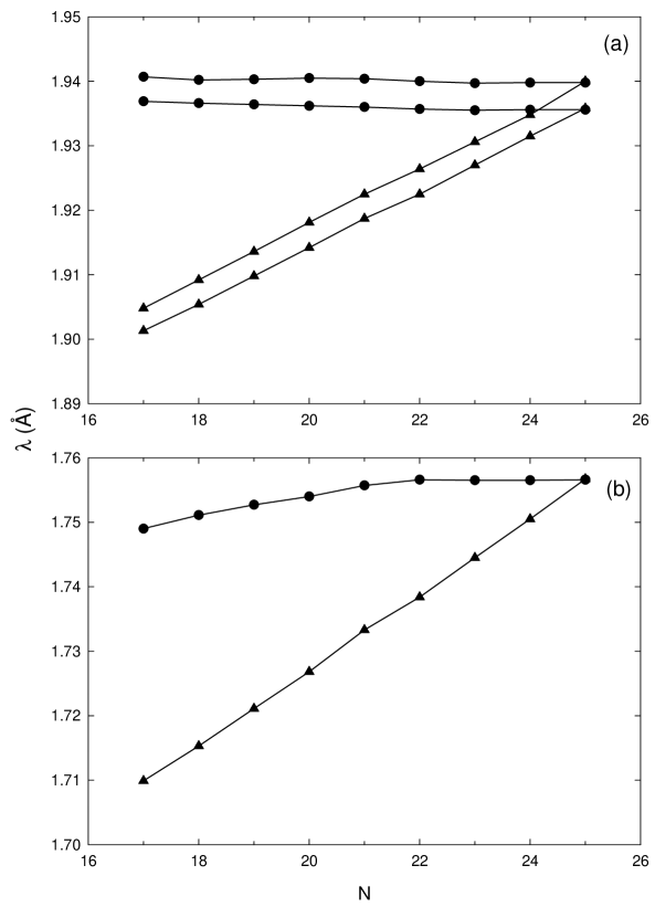
Figure 1: Comparison of centroid wavelengths for (a) K$\alpha$ and (b) K$\beta$ UTAs in Fe ions with $17\leq N\leq 25$. Filled circles: this work. Filled triangles: Kaastra & Mewe (1993).

Table 1: Comparison of centroid wavelengths (Å) for the K$\alpha$ and K$\beta$ unresolved transition arrays in Fe ions with $17\leq N\leq 25$. The hfr wavelengths have been weighted with the fluorescence yields. Experimental wavelengths for Fe x ($N=17$) are from Decaux et al. (1995) and for solid-state iron from Hölzer et al. (1997).

	HFR			Expt
$N$	K$\alpha$	K$\beta$		K$\alpha$	K$\beta$
17	1.9369	1.7488		1.9388(5)
	1.9407	1.7493		1.9413(5)
18	1.9366	1.7511
	1.9402
19	1.9364	1.7527
	1.9403
20	1.9362	1.7540
	1.9405
21	1.9360	1.7557
	1.9404
22	1.9357	1.7566
	1.9400
23	1.9355	1.7565
	1.9397
24	1.9356	1.7565
	1.9398
25	1.9356	1.7566		1.936041(3)	1.756604(4)
	1.9398			1.939973(3)

Centroid wavelengths for the K$\alpha$ and K$\beta$ unresolved transition arrays (UTAs) computed with hfr are presented in Table 1, including also a comparison with experiment. For the K$\alpha_{1}$ and K$\alpha_{2}$ lines, it can be seen that the agreement with the solid-state measurements by Hölzer et al. (1997) ($\sim 0.5$ mÅ) is somewhat better than that with the EBIT results for Fe x (Decaux et al. 1995) of within 2 mÅ, and the slight blueshift with increasing $N$ predicted by hfr is consistent with experiment. A small redshift with $N$ is also found for the K$\beta$ array. On the other hand, as shown in Figure 1, the present findings contrast with the steeper redshift for both UTAs obtained from the data by Kaastra & Mewe (1993).

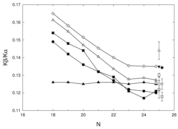
Figure 2: Comparison of K$\beta$/K$\alpha$ intensity ratios for Fe ions with $18\leq N\leq 25$. Filled circles: hfr, this work. Dotted upright triangles: autostructure, this work. Dotted diamonds: mcdf-sal, this work. Filled upright triangles: Kaastra & Mewe (1993). Filled squares: Jacobs & Rozsnyai (1986). Filled diamonds: Scofield (1974). Filled inverted triangles: Jankowski & Polasik (1989). Circles: Perujo et al. (1987). Upright triangles: Hölzer et al. (1997). Squares: Rao et al. (1986). Diamonds: Berényi et al. (1978). Inverted triangles: Salem et al. (1972). Dotted circles: Slivinsky & Ebert (1972). Dotted squares: Hansen et al. (1970).

Table 2: Comparison of hfr K$\alpha_{2}$/K$\alpha_{1}$ ratios for Fe ions ($18\leq N\leq 25$) with experiment and previous theoretical estimates.

$N$	Ion	HFR1a	HFR2 b	Expt.	Theory
18	Fe ix	0.7000	0.5912
19	Fe viii	0.5780	0.6015
20	Fe vii	0.4541	0.5821
21	Fe vi	0.5545	0.5538
22	Fe v	0.5852	0.5346
23	Fe iv	0.4426	0.5143
24	Fe iii	0.4438	0.5032
25	Fe ii	0.4476	0.4969	0.51(2)c	0.5107g
				0.507(10)d
				0.506e
				0.4998f

• Includes only the decay lines from the K-vacancy levels listed in Table 3
  

• Includes all the decay lines from the $[{\rm 1s}]({\rm 3d+4s})^{M+1}$ complex
  

• Hölzer et al. (1997)
  

• McGrary et al. (1971)
  

• Salem & Wimmer (1970)
  

• Williams (1933)
  

• Scofield (1974)
  

In Table 2, K$\alpha_{2}$/K$\alpha_{1}$ intensity ratios are tabulated for different ionization stages. Two cases have been considered: HFR1, only the decay lines from the K-vacancy levels populated by the photoionization of the respective ground state are included; and HFR2, all the transitions from the levels belonging to the $[{\rm 1s}]({\rm 3d+4s})^{M+1}$ complex are taken into account. Noticeable differences in the ratios from these two cases may be appreciated indicating sensitivity to the excitation mechanism. The HFR2 ratio for Fe ii is closer to the Dirac–Fock value of Scofield (1974), who also considered all the K-vacancy states, and to the solid-state experiments (Hölzer et al. 1997; McGrary et al. 1971; Salem & Wimmer 1970; Williams 1933).

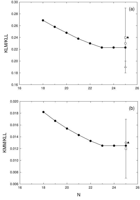
Figure 3: Comparison of Auger rates for Fe ions with $18\leq N\leq 25$: (a) KLM/KLL and (b) KMM/KLL ratios. Filled circles: hfr, this work. Upright filled triangles: Chen et al. (1979). Circles: Bhalla & Ramsdale (1970). Squares: Kovalík et al. (1987). Upright triangles: Mehlhorm & Albridge (1963).

In Figure 2, theoretical and experimental K$\beta$/K$\alpha$ intensity ratios are plotted as a function of electron number. Most experimental ratios (Rao et al. 1986; Berényi et al. 1978; Salem et al. 1972; Slivinsky & Ebert 1972; Hansen et al. 1970) have been scaled down by 8.8% in order to extract the radiative-Auger (5%) and K$\beta_{5}$ (3.8%) satellite contributions from the K$\beta$ UTA which theory does not include (Verma 2000). The value quoted in Perujo et al. (1987) does not take into account the blend with the K$\beta_{5}$ satellite and has been corrected accordingly. With the exception of the values by Kaastra & Mewe (1993), theory predicts a decrease of the ratio with $N$, and the theoretical scatter is comparable with that among the solid-state experiments of just under 20%. The computed results by hfr, autostructure and Jacobs & Rozsnyai (1986) for $N=25$ are in good agreement with the bulk of the experimental values (Perujo et al. 1987; Rao et al. 1986; Berényi et al. 1978; Salem et al. 1972; Slivinsky & Ebert 1972; Hansen et al. 1970). Hölzer et al. (1997) mention a possible systematic deviation in one of their corrections to explain the discrepancy of their data with other measurements. On the other hand, the Dirac–Fock ratios by Scofield (1974) and Jankowski & Polasik (1989) at $N=25$ appear significantly higher. We have therefore proceeded to verify these values by using the same code (mcdf-sal) as in Jankowski & Polasik (1989), and as shown in Figure 2, they are accurately reproduced; moreover, a similar decrease in the ratio with $N$ is also obtained with this method. The spread of the different data sets in this comparison indicates a probable accuracy of our hfr transition probabilities of $\sim 10\%$.

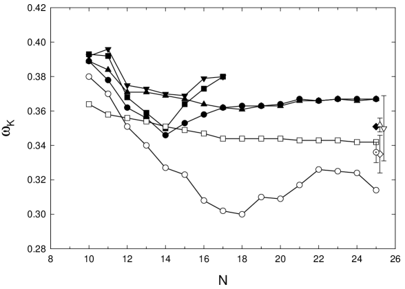
Figure 4: Comparison of K-shell fluorescence yields, $\omega_{K}$, for Fe ions $10\leq N\leq 25$. Filled circles: hfr value obtained for the first K-vacancy level, $10\leq N\leq 17$ (Paper III), $18\leq N\leq 25$ (this work). Filled squares: autostructure value obtained for the first K-vacancy level, Paper III. Filled upright triangle: hfr value obtained by averaging on all the K-vacancy levels, $10\leq N\leq 17$ (Paper III), $18\leq N\leq 25$ (this work). Filled inverted triangle: autostructure value obtained by averaging on all the K-vacancy levels, Paper III. Circles: Jacobs & Rozsnyai (1986). Squares: Kaastra & Mewe (1993). Filled diamonds: value recommended by Hubbell et al. (1994). Upright triangle: Solé (1992). Inverted triangle: Pious et al. (1992). Diamond: Bhan et al. (1981). Dotted circle: Singh et al. (1990).

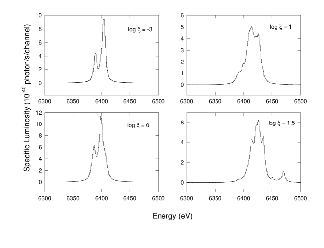
Figure 5: Simulations carried out near 6.4 keV with the xstar modeling code for several values of the ionization parameter $\xi$.

A decrease with $N$ is also predicted by hfr for the Auger KLM/KLL and KMM/KLL ratios (see Figure 3). For Fe ii, present results are in excellent accord with the measurements of Kovalík et al. (1987) and other theory (Chen et al. 1979; Bhalla & Ramsdale 1970) but somewhat higher than the older experimental estimate of Mehlhorm & Albridge (1963). The total K-shell fluorescence yields, $\omega_{K}$, for Fe ions with $10\leq N\leq 25$ are presented in Figure 4. In both hfr and autostructure data sets, the fluorescence yields have been computed for fine-structure K-vacancy levels:

$$\omega_{K}(i)\leavevmode\nobreak\ =\leavevmode\nobreak\ \frac{A_{r}(i)}{A_{r}(i)+A_{a}(i)}\ .$$ (25)

In order to display the effect of the level population, we report in Figure 4 the value for the first K-vacancy level and the yield averaged over all the K-vacancy levels. As expected, the fluorescence yield is independent of the population mechanism in the third row ions where the K$\beta$, KLM and KMM decay channels become spectators. Given the complexity of level-to-level calculations of Auger rates, it has not been possible to compute fluorescence yields with autostructure for $N>17$. The most recent experimental measurements in the solid (Solé 1992; Pious et al. 1992; Singh et al. 1990; Bhan et al. 1981) are plotted along with the value recommended by Hubbell et al. (1994). They show a scatter within 10% and are slightly lower than our hfr value for $N=5$, i.e. 5 to 10% with respect to Hubbell et al. (1994) and Bhan et al. (1981) respectively. This is not a significant discord considering the expected accuracy of our fluorescence yields ($\sim 20\%$) as discussed in Paper III. As mentioned in the previous section, the missing participator Auger channels will not contribute significantly to the Auger widths (less than 1%). Concerning the shake-up channels, they will not affect the Auger widths because they are due to mixing between valence shell configurations which have the same Auger widths. We have verified that this is the case in a simple calculation ($[{\rm 1s}]({\rm 3d+4s})^{8}\rightarrow[{\rm 2p}]^{2}({\rm 3d+4s})^{8}+k{\rm s}$). Data by Kaastra & Mewe (1993) have been corrected so as to reproduce the best solid-state yields compiled in Bambynek et al. (1972) and are therefore somewhat lower than our values. Results by Jacobs & Rozsnyai (1986) for $N>12$ predict a substantially lower yield.

In order to evaluate the impact of the new atomic data on Fe K-line modeling, the data sets generated in the present work and those in Papers I–III have been included in the xstar modeling code (Kallman & Bautista 2001). Runs for different ionization parameters, $\xi$, are shown in Figure 5. The other parameters have been assigned the following values: cosmic abundances; a gas column density of $10^{16}$ cm^-2; a gas density of $10^{12}$ cm^-3; an X-ray source luminosity of 10³⁸ erg/s; a power-law index of 1; and energy bins (or channel widths) of 1 eV. In Figure 5, one clearly sees that the UTA centroid is redshifted when $\xi$ goes from 0.001 to 1 and then blueshifted for $\xi>1$. The shape of the UTA changes also considerably for $\xi>1$ where the ionization balance favors the first and second row ions.

Electronic Tables 3–4 list radiative and Auger widths for 295 energy levels; and wavelengths, $A$-values and fluorescence yields for 396 transitions.

5 Summary and conclusions

Following the findings of our previous study on the second-row iron ions (Paper III), the hfr package (Cowan 1981) has been selected to compute level energies, wavelengths, decay rates and fluorescence yields for the K-vacancy states in Fe ii–Fe ix. The calculations have focused states populated by ground-state photoionization. Due to the complexity of the level-to-level Auger calculations, we have employed a compact formula (Palmeri et al. 2001) to compute Auger widths from the hfr radial integrals.

The hfr centroid wavelengths for the K$\alpha$ and K$\beta$ UTAs in Fe ii reproduce the solid-state measurements (Hölzer et al. 1997) to better than 1 mÅ. Moreover, the red shift predicted by hfr for the K$\alpha$ lines in species with higher ionization stage is in accord with the EBIT wavelengths in Fe x (Decaux et al. 1995) thus contradicting the previous trend specified by Kaastra & Mewe (1993). We have also carried out extensive comparisons of different hfr branching ratios, namely K$\alpha_{2}$/K$\alpha_{1}$, K$\beta$/K$\alpha$, KLM/KLL, KMM/KLL and $\omega_{K}$, with other theoretical and experimental data. The present ratios for Fe ii are in good agreement with the solid-state measurements, and the K$\alpha_{2}$/K$\alpha_{1}$ ratio has been found to be sensitive to the excitation mechanism. It has been possible from these comparisons to estimate an accuracy of $\sim$10% for the hfr transition probabilities.

The new atomic data sets for the whole Fe isonuclear sequence that have emerged from the present project are providing a more reliable platform for the modeling of Fe K lines. Preliminary simulations of the emissivity of a photoionized gas with xstar (Kallman & Bautista 2001) have shown K$\alpha$ line profiles and wavelength shifts that are sensitive to the ionization level of the gas. Further work will therefore be concerned with improving diagnostic capabilities by means of accurate K-shell photoionization and electron impact excitation cross sections.