Decay Properties of K-Vacancy States in Fe x–Fe xvii

We report extensive calculations of the decay properties of fine-structure K-vacancy levels in Fe x–Fexvii. A large set of level energies, wavelengths, radiative and Auger rates, and fluorescence yields has been computed using three different standard atomic codes, namely Cowan’s hfr, autostructure and the Breit–Pauli R-matrix package. This multi-code approach is used to the study the effects of core relaxation, configuration interaction and the Breit interaction, and enables the estimate of statistical accuracy ratings. The K$\alpha$ and KLL Auger widths have been found to be nearly independent of both the outer-electron configuration and electron occupancy keeping a constant ratio of $1.53\pm 0.06$. By comparing with previous theoretical and measured wavelengths, the accuracy of the present set is determined to be within 2 mÅ. Also, the good agreement found between the different radiative and Auger data sets that have been computed allow us to propose with confidence an accuracy rating of 20% for the line fluorescence yields greater than 0.01. Emission and absorption spectral features are predicted finding good correlation with measurements in both laboratory and astrophysical plasmas.

1 Introduction

The iron K lines appear in a relatively unconfused spectral region and have a high diagnostic potential. The study of these lines has been encouraged by the quality spectra emerging from Chandra and by the higher resolution expected from Astro-E and Constellation-X. In addition there is a shortage of accurate and complete level-to-level atomic data sets for the K-vacancy states of the Fe isonuclear sequence, in particular for the lowly ionized species. This undermines line identification and realistic spectral modeling. We are currently remedying this situation by systematic calculations using suites of codes developed in the field of computational atomic physics. Publicly available packages have been chosen rather than in-house developments. In this context, complete data sets for the $n=2$ K-vacancy states of the first row, namely Fe xviii–Fe xxv, have been reported earlier by Bautista et al. (2003) and Palmeri et al. (2003), to be referred to hereafter as Paper I and Paper II.

In spite of diagnostic possibilities in non-equilibrium ionization conditions and photoionized plasmas, the K lines from Fe species with electron occupancies $N>10$ have been hardly studied. This is perhaps due to the greater spectral complexity arising from the open 3p and 3d subshells that makes a formal rendering of their radiative and Auger decay pathways a daunting task. Decaux et al. (1995) have made laboratory wavelength measurements of some of these lines, and compare with the theoretical predictions obtained with the hullac code (Klapisch et al. 1977; Bar-Shalom et al. 1988), based on a relativistic multiconfiguration parametric potential model, and with the multiconfiguration Dirack–Fock package known as grasp (Grant et al. 1980). However, no decay rates are reported by Decaux et al. (1995). In earlier work, Jacobs & Rozsnyai (1986) compute fluorescence probabilities in a frozen-cores approximation for vacancies among the $nl$ subshells of the Fe isonuclear sequence, but ignore multiplets and fine-structure.

The present report is concerned with a detailed study of the radiative and Auger de-excitation channels of the K-shell vacancy states in the second-row species Fe x–Fe xvii. Energy levels, wavelengths, $A$-values, Auger rates, and K$\alpha$/K$\beta$ fluorescence yields have been computed for the fine-structure levels in K-vacancy configurations of the type ${\rm 1s2s}^{2}{\rm 2p}^{6}\mu$, where $\mu$ is taken to be the lowest outer electron configuration of each ion. The multi-code approach described in Paper I is employed, and attempts are made to characterize the extent of configuration interaction (CI), core relaxation effects (CRE), relativistic corrections, the dominant channels in the decay manifolds and the emergent spectral signatures. In Section 2 the numerical methods are briefly described. Section 3 contains an outline of the decay trees of the second-row Fe K-vacancy states. Results and findings are given in Sections 4–6, the spectral signatures are discussed in Section 7 and $n{\rm p}$-satellite lines are investigated in Section 8, ending with a summary and conclusions in Section 9. Finally, the complete atomic data sets for the 251 energy levels and the 876 transitions considered in this work are respectively listed in the electronic Tables 3 and 4.

2 Numerical methods and ion models

As discussed in Paper II, we adopt standard atomic physics codes, namely autostructure, bprm and hfr rather than in-house developments. We have found that their combined use compensates for individual weaknesses and provides physical insight and statistical measures. Radiative and collitional data are computed for $N$- and $(N+1)$-electron systems with the relativistic Breit–Pauli framework

$$H_{\rm bp}=H_{\rm nr}+H_{\rm 1b}+H_{\rm 2b}$$ (1)

where $H_{\rm nr}$ is the usual non-relativistic Hamiltonian. The one-body relativistic operators

$$H_{\rm 1b}=\sum_{n=1}^{N}f_{n}({\rm mass})+f_{n}({\rm d})+f_{n}({\rm so})$$ (2)

represent the spin–orbit interaction, $f_{n}({\rm so})$, and the non-fine structure mass-variation, $f_{n}({\rm mass})$, and one-body Darwin, $f_{n}({\rm d})$, corrections. The two-body corrections

$$H_{\rm 2b}=\sum_{n>m}g_{nm}({\rm so})+g_{nm}({\rm ss})+g_{nm}({\rm css})+g_{nm}({\rm d})+g_{nm}({\rm oo})\ ,$$ (3)

usually referred to as the Breit interaction, include, on the one hand, the fine structure terms $g_{nm}({\rm so})$ (spin–other-orbit and mutual spin–orbit) and $g_{nm}({\rm ss})$ (spin–spin), and on the other, the non-fine structure terms: $g_{nm}({\rm css})$ (spin–spin contact), $g_{nm}({\rm d})$ (Darwin) and $g_{nm}({\rm oo})$ (orbit–orbit).

The numerical methods are detailed in Paper I and Paper II but a brief summary is given below.

2.1 autostructure

autostructure by Badnell (1986, 1997) is an extended and revised version of the atomic structure code superstructure (Eissner et al. 1974). It computes relativistic fine structure level energies, radiative transition probabilities and autoionization rates. CI wavefunctions are constructed from an orthogonal orbital basis generated in a statistical Thomas–Fermi–Dirac potential (Eissner & Nussbaumer 1969), and continuum wavefunctions are obtained in a distorted-wave approximation. The Breit–Pauli implementation includes to order $\alpha^{2}Z^{4}$ the one- and two-body operators (fine and non-fine structure) of Eqs. (2–3) where $\alpha$ is the fine structure constant and $Z$ the atomic number. In the present study, orthogonal orbital sets are obtained by minimizing the sum of all the terms in the ion representations, i.e. those that give rise to radiative and Auger decay channels. CI is limited to the $n=3$ complex and excludes configurations with 3d orbitals. No fine tuning is introduced due to total absence of spectroscopic measurements. This approximation is hereafter referred to as AST1. A second approximation, AST2, is also considered where the orbitals for the K-vacancy states are optimized separately from those of the valence states. Although AST2 cannot be used to compute radiative or Auger rates, it provides estimates of CRE and more accurate wavelengths.

2.2 hfr

In the hfr code (Cowan 1981), an orbital basis is obtained for each electronic configuration by solving the Hartree–Fock equations for the spherically averaged atom. The equations are obtained from the application of the variational principle to the configuration average energy and include relativistic corrections, namely the Blume–Watson spin–orbit, mass–velocity and the one-body Darwin terms. The eigenvalues and eigenstates thus obtained are used to compute the wavelength and $A$-value for each possible transition. Autoionization rates are calculated in a perturbation theory scheme where the radial functions of the initial and final states are optimized separately, and CI is accounted for only in the autoionizing state. Two ion models are considered: in HFR1 the ion is modeled with a frozen-orbital basis optimized on the energy of the ground configuration while in HFR2 an orbital basis is optimized separately for each configuration by minimizing its average energy. Therefore, the different orbital bases used in HFR2 for the entire multiconfigurational model are non-orthogonal. In both approximations CI is taken into account within the $n=3$ complex, but configurations with 3d orbitals are again excluded.

2.3 bprm

The Breit–Pauli $R$-matrix method (bprm) is based on the close-coupling approximation (Burke & Seaton 1971) whereby the wavefunctions for states of the $N$-electron target and a collision electron are expanded in terms of the target eigenfunctions. The Kohn variational principle gives rise to a set of coupled integro-differential equations that are solved in the inner region ($r\leq a$, say) by $R$-matrix techniques (Burke et al. 1971; Berrington et al. 1974, 1978, 1987). In the asymptotic region ($r>a$), resonance positions and widths are obtained from fits of the eigenphase sums with the stgqb module developed by Quigley & Berrington (1996) and Quigley et al. (1998). Normalized partial widths are defined from projections onto the open channels. The Breit–Pauli relativistic corrections have been introduced in the $R$-matrix suite by Scott & Burke (1980) and Scott & Taylor (1982), but the two-body terms (see Eq. 3) have not as yet been incorporated. The target approximations adopted here, to be denoted hereafter as BPR1, include all the levels that span the complete KLL, KLM and KMM Auger decay manifold of the K-vacancy configurations of interest. For the more complicated ions this approach implies very large calculations, some of which proved intractable.

3 Decay trees

The radiative and Auger decay manifolds of a K-vacancy state $[{\rm 1s}]\mu$, where $[n\ell]$ denotes a hole in the $n\ell$ subshell and $\mu$ an M-shell configuration, can be outlined as follows:

• Radiative channels

  $$[{\rm 1s}]\mu \stackrel{{\scriptstyle{\rm K}\beta}}{{\longrightarrow}} [\mu]+\gamma_{\beta}$$ (4)

  $$\stackrel{{\scriptstyle{\rm K}\alpha}}{{\longrightarrow}} [{\rm 2p}]\mu+\gamma_{\alpha}$$ (5)

• Auger channels

  $$[{\rm 1s}]\mu \stackrel{{\scriptstyle\rm KMM}}{{\longrightarrow}} [\mu]^{2}+e^{-}$$ (6)

  $$\stackrel{{\scriptstyle\rm KLM}}{{\longrightarrow}} \left\{\begin{array}[]{l}\left[{\rm 2s}\right][\mu]+e^{-}\\ \left[{\rm 2p}\right][\mu]+e^{-}\end{array}\right\}$$ (9)

  $$\stackrel{{\scriptstyle\rm KLL}}{{\longrightarrow}} \left\{\begin{array}[]{l}\left[{\rm 2s}\right]^{2}\mu+e^{-}\\ \left[{\rm 2s}\right]\left[{\rm 2p}\right]\mu+e^{-}\\ \left[{\rm 2p}\right]^{2}\mu+e^{-}\end{array}\right\}$$ (13)

In the radiative channels, forbidden and two-electron transitions have been excluded as it has been confirmed by calculation that they display very small transition probabilities ($\log A_{\rm r}<11$). Therefore, the two main photo-decay pathways are characterized by the $2{\rm p}\rightarrow{\rm 1s}$ and $3{\rm p}\rightarrow{\rm 1s}$ single-electron jumps that give rise respectively to the K$\alpha$ ($\sim{\lambda}1.93$) and K$\beta$ ($\sim{\lambda}1.72$) arrays. After similar numerical verifications, the shake-up channels in the KLL Auger mode, where the final outer-electron configuration $\mu$ is different from the initial, are not taken into account. Of primary interest in the present work is to establish the branching ratios of the KMM, KLM and KLL Auger channels and their variations with electron occupancy $N$.

Table 1: Differences in average energies (eV) for the $[{\rm 1s}]\mu$ configurations in Fe ions ($11\leq N\leq 17$) computed in approximations HFR1, HFR2, AST1 and AST2 (see Section 2). Such differences are due to CRE.

$N$	$\mu$	$\Delta E^{\mathrm{a}}$	$\Delta E^{\mathrm{b}}$	$\Delta E^{\mathrm{c}}$
11	${\rm 3s}^{2}$	21.1	15.8	2.6
12	${\rm 3s}^{2}{\rm 3p}$	21.6	16.5	2.8
13	${\rm 3s}^{2}{\rm 3p}^{2}$	22.3	16.5	2.9
14	${\rm 3s}^{2}{\rm 3p}^{3}$	23.0	17.8	3.0
15	${\rm 3s}^{2}{\rm 3p}^{4}$	23.7	18.5	3.3
16	${\rm 3s}^{2}{\rm 3p}^{5}$	24.5	20.4	3.3
17	${\rm 3s}^{2}{\rm 3p}^{6}$	25.2	22.9	3.5

Table 2: Comparison of present theoretical wavelengths (HFR2 and AST2) for the $(N,\mu;k,i)$ K$\alpha$ transitions in Fe ions ($10\leq N\leq 17$). The HULLAC (HULL) and GRASP (GRAS) results are from Decaux et al. (1995) (see Section 4) who only report measurements for $\lambda(17,{\rm 3s}^{2}{\rm 3p}^{6};\ ^{2}{\rm S}_{1/2},\ ^{2}{\rm P}^{\rm o}_{3/2})=1.9388(5)$ Å and $\lambda(17,{\rm 3s}^{2}{\rm 3p}^{6};\ ^{2}{\rm S}_{1/2},\ ^{2}{\rm P}^{\rm o}_{1/2})=1.9413(5)$ Å. This comparison suggests that the HFR2 wavelength data set should be shifted up by 0.7 mÅ.

Transition ($N,\mu;k,i$)	$\lambda$ (Å)
	HFR2	AST2	HULL	GRAS
$(10,{\rm 3s};\ ^{3}{\rm S}_{1},\ ^{3}{\rm P}^{\rm o}_{2})$	1.9273	1.9278	1.9280	1.9280
$(10,{\rm 3s};\ ^{3}{\rm S}_{1},\ ^{1}{\rm P}^{\rm o}_{1})$	1.9279	1.9283	1.9286	1.9286
$(10,{\rm 3s};\ ^{3}{\rm S}_{1},\ ^{3}{\rm P}^{\rm o}_{0})$	1.9311	1.9315	1.9317	1.9318
$(10,{\rm 3s};\ ^{3}{\rm S}_{1},\ ^{3}{\rm P}^{\rm o}_{1})$	1.9315	1.9319	1.9321	1.9322
$(10,{\rm 3s};\ ^{1}{\rm S}_{0},\ ^{1}{\rm P}^{\rm o}_{1})$	1.9263	1.9270	1.9270	1.9269
$(10,{\rm 3s};\ ^{1}{\rm S}_{0},\ ^{3}{\rm P}^{\rm o}_{1})$	1.9299	1.9305	1.9305	1.9305
$(11,{\rm 3s}^{2};\ ^{2}{\rm S}_{1/2},\ ^{2}{\rm P}^{\rm o}_{3/2})$	1.9285	1.9291	1.9293	1.9292
$(11,{\rm 3s}^{2};\ ^{2}{\rm S}_{1/2},\ ^{2}{\rm P}^{\rm o}_{1/2})$	1.9323	1.9328	1.9330	1.9329
$(12,{\rm 3s}^{2}{\rm 3p};\ ^{3}{\rm P}^{\rm o}_{0},\ ^{3}{\rm S}_{1})$	1.9297	1.9302	1.9305	1.9304
$(12,{\rm 3s}^{2}{\rm 3p};\ ^{3}{\rm P}^{\rm o}_{0},\ ^{3}{\rm D}_{1})$	1.9341	1.9345	1.9348	1.9347
$(12,{\rm 3s}^{2}{\rm 3p};\ ^{3}{\rm P}^{\rm o}_{1},\ ^{3}{\rm S}_{1})$	1.9296	1.9301	1.9303	1.9303
$(12,{\rm 3s}^{2}{\rm 3p};\ ^{3}{\rm P}^{\rm o}_{1},\ ^{3}{\rm D}_{2})$	1.9303	1.9308	1.9311	1.9310
$(12,{\rm 3s}^{2}{\rm 3p};\ ^{3}{\rm P}^{\rm o}_{1},\ ^{3}{\rm D}_{1})$	1.9340	1.9344	1.9346	1.9346
$(12,{\rm 3s}^{2}{\rm 3p};\ ^{3}{\rm P}^{\rm o}_{1},\ ^{1}{\rm S}_{0})$	1.9392	1.9397	1.9404	1.9410
$(13,{\rm 3s}^{2}{\rm 3p}^{2};\ ^{4}{\rm P}_{1/2},\ ^{4}{\rm P}^{\rm o}_{3/2})$	1.9316	1.9321	1.9325	1.9323
$(13,{\rm 3s}^{2}{\rm 3p}^{2};\ ^{4}{\rm P}_{1/2},\ ^{2}{\rm P}^{\rm o}_{1/2})$	1.9397	1.9402	1.9412	1.9410
$(17,{\rm 3s}^{2}{\rm 3p}^{6};\ ^{2}{\rm S}_{1/2},\ ^{2}{\rm P}^{\rm o}_{3/2})$	1.9369	1.9376	1.9379	1.9379
$(17,{\rm 3s}^{2}{\rm 3p}^{6};\ ^{2}{\rm S}_{1/2},\ ^{2}{\rm P}^{\rm o}_{1/2})$	1.9407	1.9413	1.9415	1.9416

4 Energy levels and wavelengths

As discussed in Paper I and Paper II, one of the first issues to address in the calculation of atomic data for K-vacancy states is orbital choice, specially in the context of CRE. It is expected that such effects increase with $N$, and have been shown to be important in neutrals (Martin & Davidson 1977; Mooney et al. 1992). hfr is particularly effective for this task as it allows the use of non-orthogonal orbital bases that are generated by minimizing configuration average energies. This is also possible in autostructure although rates can only be computed with orthogonal orbital sets. As reported in Paper I, Auger processes in an $N$-electron ion are more accurately represented in autostructure with orbitals of the ($N-1$)-electron residual ion.

Table 5: Relativistic and non-relativistic $A$-values (s^-1) and $f$-values computed in approximation AST1 for the $(N,\mu;k,i)$ K$\alpha$ multiplet transitions in Fe xvii and Fe xiv. Note: $a\pm b\equiv a\times 10^{\pm b}$.

					Non-relativistic				Relativistic
Ion	$N$	$\mu$	$k$	$i$	$\lambda$ (Å)	$A_{\alpha}(k,i)$	$f(i,k)$		$\lambda$ (Å)	$A_{\alpha}(k,i)$	$f(i,k)$
Fe xvii	10	${\rm 3s}$	${}^{3}{\rm S}$	${}^{3}{\rm P}^{\rm o}$	1.944	5.71$+$14	1.08$-$1		1.931	5.04$+$14	9.31$-$2
		${\rm 3s}$	${}^{1}{\rm S}$	${}^{1}{\rm P}^{\rm o}$	1.944	5.72$+$14	1.08$-$1		1.929	3.38$+$14	6.24$-$2
		${\rm 4s}$	${}^{3}{\rm S}$	${}^{3}{\rm P}^{\rm o}$	1.943	5.72$+$14	1.08$-$1		1.930	5.19$+$14	9.58$-$2
		${\rm 4s}$	${}^{1}{\rm S}$	${}^{1}{\rm P}^{\rm o}$	1.943	5.74$+$14	1.08$-$1		1.928	3.79$+$14	6.99$-$2
		${\rm 5s}$	${}^{3}{\rm S}$	${}^{3}{\rm P}^{\rm o}$	1.943	5.72$+$14	1.08$-$1		1.930	5.23$+$14	9.64$-$2
		${\rm 5s}$	${}^{1}{\rm S}$	${}^{1}{\rm P}^{\rm o}$	1.943	5.71$+$14	1.08$-$1		1.928	3.85$+$14	7.10$-$2
		${\rm 3p}$	${}^{3}{\rm P}^{\rm o}$	${}^{3}{\rm D}$	1.945	3.19$+$14	1.08$-$1		1.930	3.12$+$14	1.04$-$1
				${}^{3}{\rm P}$	1.945	1.89$+$14	1.07$-$1		1.932	1.26$+$14	7.00$-$2
				${}^{3}{\rm S}$	1.943	6.30$+$13	1.07$-$1		1.929	6.23$+$13	1.03$-$1
		${\rm 3p}$	${}^{1}{\rm P}^{\rm o}$	${}^{1}{\rm D}$	1.944	3.17$+$14	1.08$-$1		1.933	1.53$+$14	5.10$-$2
				${}^{1}{\rm P}$	1.944	1.92$+$14	1.09$-$1		1.929	1.19$+$14	6.59$-$2
				${}^{1}{\rm S}$	1.951	5.54$+$13	9.48$-$1		1.938	4.37$+$13	7.32$-$2
Fe xiv	13	${\rm 3s}^{2}{\rm 3p}^{2}$	$(^{1}{\rm S})\ ^{2}{\rm S}$	$(^{3}{\rm P})\ ^{2}{\rm P}^{\rm o}$	1.946	3.40$+$13	6.44$-$3		1.936	1.59$+$13	2.93$-$3
				$(^{1}{\rm S})\ ^{2}{\rm P}^{\rm o}$	1.949	4.99$+$14	9.48$-$2		1.937	4.06$+$14	7.54$-$2
				$(^{1}{\rm D})\ ^{2}{\rm P}^{\rm o}$	1.953	2.73$+$13	5.19$-$3		1.939	9.15$+$13	1.71$-$2

In Table 1 the differences in average energy computed in HFR1 (orthogonal orbitals) and HFR2 (non-orthogonal orbitals) for the $[{\rm 1s}]\mu$ configurations in Fe ions with $11\leq N\leq 17$ are tabulated. It may be seen that they are larger than 20 eV and grow with $N$. They are comparable with those resulting between AST1 and AST2 (see Table 1) but slightly larger due to the orbital optimization procedure in autostructure that involves the complete level set in the ion representation rather than just the ground state as in HFR1 (see Section 2). These sizable discrepancies are caused by CRE, a fact that has led us to choose HFR2 as our production model.

HFR2 and AST2 wavelengths for the $[{\rm 1s}]\mu(k)\rightarrow[{\rm 2p}]\mu(i)$ K$\alpha$ transitions in Fe ions with $10\leq N\leq 17$ are compared in Table 2 with the theoretical values reported by Decaux et al. (1995). The latter have been calculated with the code hullac based on a relativistic multiconfiguration parametric potential method (Klapisch et al. 1977; Bar-Shalom et al. 1988) and with the multiconfiguration Dirac–Fock code grasp (Grant et al. 1980). No details are given on their orbital optimization procedure. The HFR2 data are found to be systematically shorter by an average of $0.8\pm 0.3$ mÅ. Decaux et al. (1995) also present measurements performed with an electron beam ion trap for the $(N,\mu;k,i)\equiv(10,{\rm 3s}^{2}{\rm 3p}^{6};\ ^{2}{\rm S}_{1/2},\ ^{2}{\rm P}^{\rm o}_{J})$ K$\alpha$ doublet in Fe x at 1.9388(5) Å and 1.9413(5) Å where again the HFR2 values are smaller by 1.9 mÅ and 0.6 mÅ, respectively. Moreover, HFR2 values are below AST2 by an average of $0.5\pm 0.1$ mÅ (see Table 2). The present comparison indicates that the HFR2 ab initio wavelengths can be improved by shifting them up by 0.7 mÅ. The good agreement between AST2, hullac, and grasp data sets suggests that this small shift is caused by the incomplete implementation of the Breit interaction in hfr. However, as CRE is expected to affect rates much more than the Breit interaction, HFR2 is still our prefered approach. On the other hand, the theoretical energy splittings for the $[{\rm 2p}]{\rm 3s}^{2}{\rm 3p}^{6}\ {}^{2}{\rm P}^{\rm o}_{J}$ levels of Fe x are noticeably consistent: the average value is equal to $(9.8\pm 0.2)\times 10^{4}$ cm^-1 which is significantly different from the value of $6.64\times 10^{4}$ cm^-1 derived from the experimental wavelengths.

For each ion, we have only considered the radiative decay tree of the fine-structure states in the lowest K-vacancy configuration, except for Fe xvii and Fe xvi where the first excited configuration has also been included. A complete data set that lists configuration assignments and HFR2 energies for the 251 levels involved is given in the electronic Table 3. The 876 HFR2 transition wavelengths (shifted up by 0.7 mÅ) for both the K$\alpha$ and K$\beta$ arrays are listed in the electronic Table 4.

5 Radiative decay

In order to bring out the radiative decay properties of the K-vacancy states in Fe ions with filled L shells, we compute with autostructure relativistic and non-relativistic $A$- and $f$-values for the $[{\rm 1s}]\mu(k)\rightarrow[{\rm 2p}]\mu(i)$ K$\alpha$ multiplets involving the $[{\rm 1s}]n{\rm s}$ and $[{\rm 1s}]{\rm 3p}$ states in Fe xvii and the $[{\rm 1s}]{\rm 3s}^{2}{\rm 3p}^{2}$ in Fe xiv. As depicted in Table 5 for the non-relativistic case,

$$A_{\alpha}(10,n{\rm s};\ ^{3}{\rm S},\ ^{3}{\rm P}^{\rm o})\approx A_{\alpha}(10,n{\rm s};\ ^{1}{\rm S},\ ^{1}{\rm P}^{\rm o})\approx 5.72\times 10^{14}{\rm s}^{-1}$$ (14)

and

$$f(10,n{\rm s};\ ^{3}{\rm P}^{\rm o},\ ^{3}{\rm S})=f(10,n{\rm s};\ ^{1}{\rm P}^{\rm o},\ ^{1}{\rm S})=0.108\ ;$$ (15)

that is, the radiative width and total absorption oscillator strength are practically independent of multiplicity and $n$. This behavior illustrates the approximate validity of Gauss’s law at the atomic scale where the spectator $n$s electron ($n>2$) does not affect the inner-shell process, and has been previously mentioned by Manson et al. (1991) in the context of the inner-shell properties of Kr and Sn.

Table 6: Relativistic $A$-values (s^-1), $f$-values and $B_{\Delta J}$ branching ratios computed in approximation AST1 for the $(N,\mu;k,i)$ fine-structure K$\alpha$ transitions in Fe xvii. Note: $a\pm b\equiv a\times 10^{\pm b}$.

$\mu$	$k$	$i$	$A_{\alpha}(k,i)$	$f(i,k)$	$B_{\Delta J}(i,k)$	$\mu$	$k$	$i$	$A_{\alpha}(k,i)$	$f(i,k)$	$B_{\Delta J}(i,k)$
3s	${}^{3}{\rm S}_{1}$	${}^{3}{\rm P}_{2}^{\rm o}$	3.29$+$14	1.09$-$1	1.000	3p	${}^{3}{\rm P}_{2}^{\rm o}$	${}^{3}{\rm D}_{1}$	1.52$+$12	1.41$-$3	0.013
		${}^{3}{\rm P}_{1}^{\rm o}$	1.10$+$14	6.12$-$2	0.561			${}^{3}{\rm P}_{1}$	8.31$+$13	7.71$-$2	0.712
		${}^{1}{\rm P}_{1}^{\rm o}$	8.63$+$13	4.78$-$2	0.439	3p	${}^{3}{\rm P}_{1}^{\rm o}$	${}^{3}{\rm D}_{2}$	2.99$+$14	9.95$-$2	0.910
		${}^{3}{\rm P}_{0}^{\rm o}$	6.53$+$13	1.09$-$1	1.000			${}^{3}{\rm P}_{2}$	2.17$+$13	7.21$-$3	0.066
3s	${}^{1}{\rm S}_{0}$	${}^{1}{\rm P}_{1}^{\rm o}$	3.38$+$14	6.24$-$2	0.562			${}^{1}{\rm D}_{2}$	7.95$+$12	2.66$-$3	0.024
		${}^{3}{\rm P}_{1}^{\rm o}$	2.62$+$14	4.86$-$2	0.438			${}^{1}{\rm P}_{1}$	4.46$+$11	2.47$-$4	0.002
4s	${}^{3}{\rm S}_{1}$	${}^{3}{\rm P}_{2}^{\rm o}$	3.29$+$14	1.09$-$1	1.000			${}^{3}{\rm S}_{1}$	7.70$+$13	4.26$-$2	0.392
		${}^{3}{\rm P}_{1}^{\rm o}$	1.24$+$14	6.91$-$2	0.634			${}^{3}{\rm D}_{1}$	1.11$+$14	6.19$-$2	0.569
		${}^{1}{\rm P}_{1}^{\rm o}$	7.21$+$13	3.99$-$2	0.366			${}^{3}{\rm P}_{1}$	7.27$+$12	4.05$-$3	0.037
		${}^{3}{\rm P}_{0}^{\rm o}$	6.54$+$13	1.09$-$1	1.000			${}^{3}{\rm P}_{0}$	4.89$+$13	8.15$-$2	0.753
4s	${}^{1}{\rm S}_{0}$	${}^{1}{\rm P}_{1}^{\rm o}$	3.79$+$14	6.99$-$2	0.636			${}^{1}{\rm S}_{0}$	1.59$+$13	2.67$-$2	0.247
		${}^{3}{\rm P}_{1}^{\rm o}$	2.16$+$14	4.00$-$2	0.364	3p	${}^{3}{\rm P}_{0}^{\rm o}$	${}^{3}{\rm S}_{1}$	2.51$+$14	4.63$-$2	0.425
5s	${}^{3}{\rm S}_{1}$	${}^{3}{\rm P}_{2}^{\rm o}$	3.29$+$14	1.09$-$1	1.000			${}^{1}{\rm P}_{1}$	1.53$+$14	2.82$-$2	0.259
		${}^{3}{\rm P}_{1}^{\rm o}$	1.28$+$14	7.10$-$2	0.651			${}^{3}{\rm D}_{1}$	1.76$+$14	3.27$-$2	0.300
		${}^{1}{\rm P}_{1}^{\rm o}$	6.89$+$13	3.81$-$2	0.349			${}^{3}{\rm P}_{1}$	9.82$+$12	1.82$-$3	0.017
		${}^{3}{\rm P}_{0}^{\rm o}$	6.54$+$13	1.09$-$1	1.000	3p	${}^{1}{\rm P}_{1}^{\rm o}$	${}^{3}{\rm D}_{2}$	2.78$+$13	9.22$-$3	0.085
5s	${}^{1}{\rm S}_{0}$	${}^{1}{\rm P}_{1}^{\rm o}$	3.85$+$14	7.10$-$2	0.652			${}^{3}{\rm P}_{2}$	1.46$+$14	4.87$-$2	0.447
		${}^{3}{\rm P}_{1}^{\rm o}$	2.05$+$14	3.79$-$2	0.348			${}^{1}{\rm D}_{2}$	1.53$+$14	5.10$-$2	0.468
3p	${}^{3}{\rm P}_{2}^{\rm o}$	${}^{3}{\rm D}_{3}$	2.77$+$14	1.10$-$1	1.000			${}^{3}{\rm S}_{1}$	8.83$+$12	4.88$-$3	0.044
		${}^{3}{\rm D}_{2}$	1.11$+$12	6.12$-$4	0.006			${}^{1}{\rm P}_{1}$	1.19$+$14	6.59$-$2	0.599
		${}^{3}{\rm P}_{2}$	9.53$+$13	5.28$-$2	0.486			${}^{3}{\rm D}_{1}$	2.44$+$13	1.35$-$2	0.123
		${}^{1}{\rm D}_{2}$	9.93$+$13	5.53$-$2	0.509			${}^{3}{\rm P}_{1}$	4.62$+$13	2.57$-$2	0.234
		${}^{1}{\rm P}_{1}$	1.66$+$13	1.53$-$2	0.141			${}^{3}{\rm P}_{0}$	1.56$+$13	2.60$-$2	0.262
		${}^{3}{\rm S}_{1}$	1.57$+$13	1.44$-$2	0.133			${}^{1}{\rm S}_{0}$	4.37$+$13	7.32$-$2	0.738

In a similar fashion, it can be seen in Table 5 that the radiative width of the $[{\rm 1s}]3{\rm p}\ ^{3}{\rm P}^{\rm o}$ in Fe xvii, in spite of displaying three $\Delta L$ branches, has a total value ($5.71\times 10^{14}$ s^-1) close to the width of the $[{\rm 1s}]n{\rm s}$ states. Each branch has the same absorption oscillator strength ($f\approx 0.107$), and the rates are approximately in the ratios of their statistical weights. The situation is somewhat different for the $[{\rm 1s}]{\rm 3p}\ ^{1}{\rm P}^{\rm o}$ level because, although the $\Delta L=1$ and $\Delta L=0$ branches have similar quantitative properties as the triplet, the $A$-value for $\Delta L=-1$ is 14% smaller; this is caused by CI between $[{\rm 2p}]3{\rm p}\ ^{1}{\rm S}$ and the ${\rm 2p}^{6}\ {}^{1}{\rm S}$ ground state. The radiative width ($5.60\times 10^{14}$ s^-1) and total absorption oscillator strength (0.106) for the single decay branch ($\Delta L=1$) of the $[{\rm 1s}]{\rm 3s}^{2}{\rm 3p}^{2}(^{1}{\rm S})\ ^{2}{\rm S}$ state in Fe xiv are not much different, but in this case there are three transitions (see Table 5) where the one with the largest $A$-value corresponds to that where the state of the outer-electron configuration (i.e. ${}^{1}{\rm S}$) does not change.

The non-relativistic picture that therefore emerges is that for second-row Fe ions the K$\alpha$ transitions give rise to a dense forest of satellite lines on the red side of the Fe xviii resonance doublet. Their radiative properties are hardly affected by the outer-electron configuration and electron occupancy, and the exchange interactions and CI play minor roles. Therefore, such K-vacancy states have radiative widths constrained by that of the $[{\rm 1s}]\ ^{2}{\rm S}$ state of the F-like ion, i.e. $5.83\times 10^{14}$ s^-1 (Palmeri et al. 2003). Likewise, their oscillator strengths obey the sum rule for each $\Delta L$ branch

$$f_{\Delta L}(k)=\sum_{i}f_{\Delta L}(i,k)$$ (16)

where $f_{\Delta L}(k)\approx 0.109$, the absorption $f$-value of the $[{\rm 2p}]\rightarrow[{\rm 1s}]$ K$\alpha$ doublet of Fe xviii (Palmeri et al. 2003).

When relativistic corrections are taken into account, it can be seen in Table 5 that the multiplet radiative data are significantly modified denoting strong level admixture. However, in spite of the mixed decay manifolds, it is shown in Table 6 that the above mentioned sum rules are essentially obeyed by each fine-structure level, instead of the $LS$ multiplet, if the intermediate-coupling selection rules are assumed; i.e. there are now three $\Delta J$ branches where

$$A_{\alpha}(k)=\sum_{\Delta J}\sum_{i}A_{\Delta J}(i,k)\approx 5.83\times 10^{14}\quad{\rm s}^{-1}$$ (17)

and

$$f_{\Delta J}(k)=\sum_{i}f_{\Delta J}(i,k)\approx 0.109\ .$$ (18)

For each $\Delta J$, transitions can be assigned the branching ratio

$$B_{\Delta J}(i,k)=\frac{f_{\Delta J}(i,k)}{\sum_{i}f_{\Delta J}(i,k)}$$ (19)

which is useful in denoting level mixing. As shown in Table 6, transitions with the larger $A$-values are, in the first place, those involving K levels with a single decay branch ($\Delta J=1$) and high $B_{\Delta J}(i,j)$, e.g. $(10,n{\rm s};\ ^{1}{\rm S}_{0},\ ^{1}{\rm P}^{\rm o}_{1})$ and $(10,3{\rm p};\ ^{3}{\rm P}^{\rm o}_{0},\ ^{3}{\rm S}_{1})$; in the second, for the case of multiple decay branches, those with $\Delta J=1$ and high $B_{\Delta J}(i,j)$, e.g. $(10,n{\rm s};\ ^{3}{\rm S}_{1},\ ^{3}{\rm P}^{\rm o}_{2})$, $(10,{\rm 3p};\ ^{3}{\rm P}^{\rm o}_{2},\ ^{3}{\rm D}_{3})$ and $(10,{\rm 3p};\ ^{3}{\rm P}^{\rm o}_{1},\ ^{3}{\rm D}_{2})$. Moreover, since branching and admixture increases notably with half-filled 3p subshells and the sum rule imposes a strict upper bound on the radiative width, Fe ions with electron occupancies $12\leq N\leq 16$ give rise to a large number of satellites, most with small rates but with the occasional strong lines where level mixing does not take place.

In Table 7 K$\alpha$ and K$\beta$ widths computed in HFR2 and AST1 are presented for ions with $10\leq N\leq 17$. As previously discussed, the near constancy of the K$\alpha$ widths is clearly manifested although there is an apparent small reduction ($\sim 6$%) with $N$. By computing the AST1 data with and without the two-body relativistic operators, it is found that the differences in the K$\alpha$ widths caused by the Breit interaction are under 1%. However, the HFR2 widths are consistently $5\pm 1$% higher than those in AST1 which we attribute to CRE. The magnitudes of the K$\beta$ widths, on the other hand, depend on the type of transitions available in the decay manifold: some levels have neglible widths while those that decay via spin-allowed channels display the larger values. The Breit interaction leads to differences in the K$\beta$ widths under 10% except for those less than $10^{13}$ s^-1 where they can be as large as 20%. The HFR2 values are again higher than those in AST1 by 9%, but on average agree to within 15%. It may be seen that the K$\beta$/K$\alpha$ width ratio never exceeds 0.25, and in general the accord between AST1 and HFR2 is within 10%. A complete set of HFR2 radiative widths is included in the electronic Table 3.

Radiative transition probabilities computed in HFR2 and AST1 are compared in Figures 1–2. As previously mentioned in Paper II, rates with $\log A_{\alpha}(k,i)<13$ are found to be very model dependent, i.e. they can change by up to orders of magnitude. For the rest, the HFR2 data are on average 5–9% larger than those in AST1 which, as previoulsy mentioned, is caused by CRE. Nonetheless, they are stable to within 20% if the transitions listed in Table 8 are excluded; such transitions are mostly affected by cancellation or by strong admixture of the lower states. HFR2 $A$-values for all transitions are tabulated in the electronic Table 4.

6 Auger decay

Auger rates have been computed in the HFR2, AST1 and BPR1 approximations and are listed in Table 9. In a similar fashion to the K$\alpha$ radiative widths and as a consequence of Gauss’s law, the KLL widths are found to be almost independent of the outer-electron configuration for each ionic species and displaying only a slight decrease ($\sim 5$%) with $N$ along the isonuclear sequence. Therefore, the $(A_{\rm KLL}:A_{\alpha})$ width ratio is expected to be constant, HFR2 predicting a value of $1.56\pm 0.02$ close to that by AST1 of $1.51\pm 0.04$. On the other hand, the KLM and KMM widths show a more pronounced increase with $N$; for instance, according to AST1 the $(A_{\rm KLL}:A_{\rm KLM}:A_{\rm KMM})$ ratio changes from $(0.925:0.071:0.004)$ in Fe xvii to $(0.768:0.216:0.017)$ in Fe x.

The inclusion of the Breit interaction in ions with $12\leq N\leq 15$ proved computationally intractable. For the others, this correction decreases the KLL, KLM and thus the total AST1 rates by approximately 5%, but the KMM components are increased by a comparable amount except for the sensitive $[{\rm 1s}]{\rm 3s3p}\ ^{4}{\rm P}$ and ${}^{2}{\rm P}$ states in Fe xvi. In particular, the ${}^{4}{\rm P}_{5/2}$ level decays in the KMM mode only via spin–spin coupling. It is also shown in Table 9 that the HFR2 KLL widths are consistently $(7\pm 2$)% larger than AST1 while the KLM are on average almost level showing a scatter under 10%. By contrast, the HFR2 KMM widths larger than $10^{12}$ s^-1 are consistently less than those in AST1 by $(10\pm 9)$%. As previously mentioned, these discrepancies can be assigned to CRE, and introduce a certain amount of error cancellation that result in a final estimated accuracy for the total HFR2 Auger widths, $A_{\rm a}$, of better than 10%.

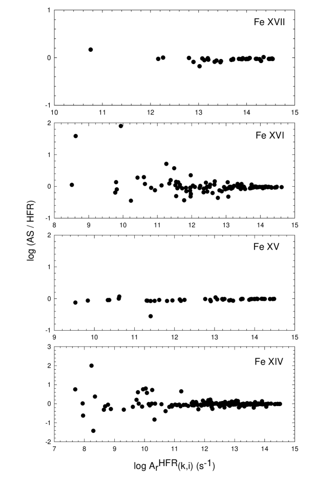
Figure 1: Comparison of transition probabilities (s^-1), $A_{r}(k,i)$, of HFR2 (HFR) and AST1 (AS) datasets for Fe xvii - xiv ions.

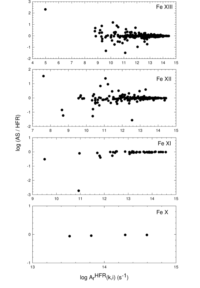
Figure 2: Comparison of transition probabilities (s^-1), $A_{r}(k,i)$, of HFR2 (HFR) and AST1 (AS) datasets for Fe xv - x ions.

BPR1 calculations of Auger rates have also been performed; they are very involved and have proved intractable for Fe ions with $N=$ 13–15. Although the BPR1 KLL widths agree with those of AST1 within 5%, differences much larger are found for the KLM and KMM widths. As explained in Paper II, it is difficult to obtain reliable partial Auger rates with bprm.

7 Spectral features

The present study of the radiative and Auger decay processes of the K-vacancy states allows us to infer some of their emission and absorption spectral features, particularly those that result from the near constancy of the total widths. Regarding the emission spectrum, we discuss the EBIT measurements in the interval 1.925–1.050 Å reported by Decaux et al. (1995). In Fig. 3 we show the wavelength intervals for the K$\alpha_{1}$ and K$\alpha_{2}$ arrays that result from the lowest K-vacancy configuration for Fe ions with effective charge, $z=Z-N+1$, in the range $1\leq z\leq 18$. They have been computed with the HFR2 model. It may be appreciated that while for ions with $z\leq 10$ two well defined peaks appear, the intermediate ions ($11\leq z\leq 17$) give rise to a dense and blended forest of satellite lines between the $[{\rm 1s}]\ ^{2}{\rm S}_{1/2}\rightarrow[{\rm 2p}]\ ^{2}{\rm P}^{\rm o}_{J}$ doublet (F1,F2) in Fe xviii and the $[{\rm 1s}]{\rm 3s}^{2}{\rm 3p}^{6}\ {}^{2}{\rm S}_{1/2}\rightarrow[{\rm 2p}]{\rm 3s}^{2}{\rm 3p}^{6}\ {}^{2}{\rm P}^{\rm o}_{J}$ doublet (Cl1,Cl2) in Fe x. This view agrees well with the laboratory spectrum: the present F and Cl doublets are estimated at (1.9268,1.9306) Å and (1.9376,1.9414) Å, respectively, compared with spectroscopic values of (1.92679,1.93079) Å and (1.9388,1.9413) Å.

The approximately constant resonance widths imply that the K$\alpha$ and K$\beta$ line fluorescence yields

$$\omega_{\alpha}(k,i)=\frac{A_{\alpha}(k,i)}{A_{\alpha}(k)+A_{\beta}(k)+A_{a}(k)}$$ (20)

and

$$\omega_{\beta}(k,i)=\frac{A_{\beta}(k,i)}{A_{\alpha}(k)+A_{\beta}(k)+A_{a}(k)}$$ (21)

are proportional to the respective $A$-value. Hence, the total level yields, $\omega_{\alpha}(k)=\sum_{i}\omega_{\alpha}(k,i)$ and $\omega_{\beta}(k)=\sum_{i}\omega_{\beta}(k,i)$, are also radiatively controled. (In the electronic Table 3, level yields are listed, and in Table 4 line yields are tabulated for all transitions; an accuracy of 20% is estimated for lines with $\omega(k,i)>0.01$.) It is therefore possible to correlate experimental spectral peaks with transitions with large $A$-values. In Table 10 transitions with $A_{\alpha}(k,i)>2.00\times 10^{14}$ s^-1 are listed. As discussed in Section 5, they all correspond to $\Delta J=1$ except for the K$\alpha_{2}$ line $(11,{\rm 3s}^{2};\ ^{2}{\rm S}_{1/2},\ ^{1}{\rm P}^{\rm o}_{1/2})$, and many involve states with $L=0$. We agree with the interpretation by Decaux et al. (1995) regarding the origin of the peaks labeled A ($\sim 1.9297$ Å) and B ($\sim 1.9322$ Å) in their EBIT spectrum, i.e. as arising respectively from ${\rm 2p}_{3/2}\rightarrow{\rm 1s}_{1/2}$ transitions in Fe xvi and Fe xiv. The transitions with the largest $A$-values in Table 10 are precisely $(11,{\rm 3s}^{2};^{2}{\rm S}_{1/2},^{2}{\rm P}^{\rm o}_{3/2})$ and $(11,{\rm 3s3p};^{2}{\rm P}^{\rm o}_{3/2},^{2}{\rm D}_{5/2})$ at 1.9292 Å and $(13,{\rm 3s}^{2}{\rm 3p}^{2};^{4}{\rm P}_{1/2},^{4}{\rm P}^{\rm o}_{3/2})$ at 1.9323 Å and $(13,{\rm 3s}^{2}{\rm 3p}^{2};^{2}{\rm S}_{1/2},^{2}{\rm P}^{\rm o}_{3/2})$ at 1.9325 Å.

The absorption features that emerge from the K-vacancy states of Fe ions have been described by Palmeri et al. (2002). The constant widths cause smeared K edges that have been observed in the X-ray spectra of active galactic nuclei and black-hole candidates (Ebisawa et al. 1994; Done & Zycki 1999). Also the K$\beta$ array gives rise to an absorption feature at $\sim 7$ KeV which has been observed but not identified in the X-ray spectra of novae and Seyfert 1 galaxies (Ebisawa et al. 1994; Pounds & Reeves 2002).

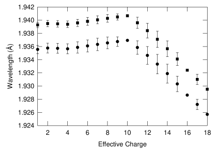
Figure 3: Wavelength intervals (depicted with error bars) for the K$\alpha_{1}$ (circles) and K$\alpha_{2}$ (squares) line arrays arising from the lowest K-vacancy configuration in Fe ions with effective charge $1\leq z\leq 18$.

8 Satellite lines

Although we have concentrated on the $n=3$ satellite lines, Palmeri et al. (2002) have predicted that the $n{\rm p}$ K-vacancy states ($n>3$) can be populated by photoabsorption. Therefore, K$\alpha$ emission feartures can be generated by the following two step processes:

• Photoexcitation followed by K$\alpha$ emission

  $$\gamma+\mu\stackrel{{\scriptstyle f}}{{\longrightarrow}}[{\rm 1s}]\mu\,n{\rm p}\stackrel{{\scriptstyle\omega_{\alpha}}}{{\longrightarrow}}[{\rm 2p}]\mu\,n{\rm p}+\gamma_{\alpha}$$ (22)

• Photoionization followed by K$\alpha$ emission

  $$\gamma+\mu\stackrel{{\scriptstyle\sigma_{\rm PI}}}{{\longrightarrow}}[{\rm 1s}]\mu+e^{-}\stackrel{{\scriptstyle\omega_{\alpha}}}{{\longrightarrow}}[{\rm 2p}]\mu+\gamma_{\alpha}+e^{-}$$ (23)

where Eqs. (22–23) respectively describe the production of the $n{\rm p}$-satellite and principal components.

In order to assess the importance of such satellite lines, shifted energies ($\Delta E=14.5$ eV), oscillator strengths and fluorescence yields have been calculated in Fe xvii for $[1s]{\rm 2p}^{6}n{\rm p}$ ($n=3-10$) Rydberg states in the AST1 approximation. The decay data in Fe xviii needed to model the main lines have been taken from Paper II. The Fe xvii photoionization cross-section of Palmeri et al. (2002) has been integrated from threshold up to 10-fold threshold to obtain the bound-free oscillator strength. In Fig. 4, each line has been modeled by a Lorentzian profile with a width equal to the depletion rate (Auger $+$ radiative widths) and an integrated intensity equal to the product of the weighted oscillator strength by the K$\alpha$ fluorescence yield. Fig. 4 clearly shows that the $n{\rm p}$-satellite lines are almost completely blended with the main lines and that they contribute less than 10% of the total intensity.

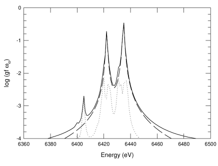
Figure 4: K$\alpha$ fluorescence lines in Fe xvii produced by photoabsorption. The product of the weighted oscillator strength ($gf$) with the fluorescence yield ($\omega_{\alpha}$) is plotted on logarithmic scale in order to enhance the faint features. The different contributions are displayed: total (solid), main lines (dash) and satellite lines (dot).

9 Summary and conclusions

As a follow-up to our previous studies on the iron K-lines (Paper I and II), we have applied the same multi-code approach to calculate level energies, wavelengths and, for the first time, radiative and Auger rates relevant to the modeling of the fluorescence properties of K-vacancy states in Fe x–Fexvii. Due to the complete lack of experimental K-excited level energies, which are used in the fine tuning of theoretical results, only ab initio data have been calculated. Systematic differences between level energies obtained with orthogonal and non-orthogonal orbital sets in both hfr and autostructure are attributed to CRE. Since hfr handles CRE more efficiently, this code is used for data production. By comparing with other theoretical data and the scarce measurements available, we have resolved to shift up the HFR wavelengths by 0.7 mÅ. The above comparison suggests that this shift is due to the incomplete implementation of the Breit interaction in hfr. However, as CRE is expected to affect much more the rates than the two-body relativistic corrections, hfr remains our prefered platform and we are confident that the hfr wavelengths are accurate to within 2 mÅ. As a result, the experimental fine-structure energy splitting of the $[{\rm 2p}]{\rm 3s}^{2}{\rm 3p}^{6}\ {}^{2}{\rm P}^{\rm o}_{J}$ term is questioned.

Radiative and Auger rates have been computed with both the HFR2 and AST1 approximations examining the effects of CI, CRE and the Breit interaction. Calculations of Auger rates with BPR1 have been also performed, but they are lengthy and for ions with $N=13-15$ proved to be intractable. The K$\alpha$ and KLL widths have been found to be nearly independent of the outer-electron configurations and electron occupancy, keeping the constant ratio $1.53\pm 0.06$. The accuracy of the HFR2 radiative rates with $\log A(k,i)>13$ has been estimated within 20% while that of the total depletion rate, $A_{\alpha}(i)+A_{\beta}(i)+A_{\rm a}(i)$, at better than 10%. While the accuracy of BPR1 KLL rates have been found to be within the latter interval, there are inherent difficulties in the current implementation to obtain reliable KLM and KMM rates. By comparing HFR2 and AST1 line fluorescence yields greater than 0.01, it has been possible to estimate their accuracy to within 20%.

The near constancy of the total depletion rates of K-vacancy states in ions with $N>9$ gives rise to characteristic spectral features which we have been able to predict and correlate with spectroscopic measurements in both laboratory and astrophysical plasmas. In this respect, we have found good quantitative agreement with the EBIT emission spectrum of Decaux et al. (1995) while the absorption features have been recently discussed by Palmeri et al. (2002).

$n{\rm p}$-Satellite lines produced by photoabsorption have been investigated. It was found that they contribute to less than 10% of the emissivity of the main lines and appear almost completely blended with them.

Finally, the HFR2 atomic data calculated for the 251 fine-structure levels and the 876 transitions considered in this study are available in two electronic tables, i.e. Tables 3 and 4 respectively.

Table 7: Radiative widths (s^-1) for states in Fe ions ($10\leq N\leq 17$) with configurations $[{\rm 1s}]\mu(i)$ computed in approximations HFR2 and AST1. Note: $a\pm b\equiv a\times 10^{\pm b}$.

			HFR2				AST1
Ion	$N$	$\mu(i)$	$A_{\alpha}(i)$	$A_{\beta}(i)$	$A_{\beta}(i)/A_{\alpha}(i)$		$A_{\alpha}(i)$	$A_{\beta}(i)$	$A_{\beta}(i)/A_{\alpha}(i)$
Fe xvii	10	${\rm 3s}\leavevmode\nobreak\ ^{3}{\rm S}_{1}$	6.26$+$14	0.00$+$00	0.00$+$00		5.88$+$14	0.00$+$00	0.00$+$00
		${\rm 3s}\leavevmode\nobreak\ ^{1}{\rm S}_{0}$	6.30$+$14	0.00$+$00	0.00$+$00		5.99$+$14	0.00$+$00	0.00$+$00
		${\rm 3p}\leavevmode\nobreak\ ^{3}{\rm P}^{\rm o}_{0}$	6.26$+$14	0.00$+$00	0.00$+$00		5.87$+$14	0.00$+$00	0.00$+$00
		${\rm 3p}\leavevmode\nobreak\ ^{3}{\rm P}^{\rm o}_{1}$	6.25$+$14	6.33$+$12	1.01$-$02		5.87$+$14	6.23$+$12	1.06$-$02
		${\rm 3p}\leavevmode\nobreak\ ^{3}{\rm P}^{\rm o}_{2}$	6.26$+$14	0.00$+$00	0.00$+$00		5.87$+$14	0.00$+$00	0.00$+$00
		${\rm 3p}\leavevmode\nobreak\ ^{1}{\rm P}^{\rm o}_{1}$	6.21$+$14	7.70$+$13	1.24$-$01		5.80$+$14	7.18$+$13	1.24$-$01
Fe xvi	11	${\rm 3s}^{2}\leavevmode\nobreak\ {}^{2}{\rm S}_{1/2}$	6.25$+$14	1.44$+$12	2.30$-$03		5.91$+$14	1.28$+$12	2.17$-$03
		${\rm 3s3p}\leavevmode\nobreak\ ^{4}{\rm P}^{\rm o}_{1/2}$	6.23$+$14	4.55$+$11	7.30$-$04		5.85$+$14	5.09$+$11	8.69$-$04
		${\rm 3s3p}\leavevmode\nobreak\ ^{4}{\rm P}^{\rm o}_{3/2}$	6.22$+$14	1.24$+$12	1.99$-$03		5.85$+$14	1.19$+$12	2.03$-$03
		${\rm 3s3p}\leavevmode\nobreak\ ^{4}{\rm P}^{\rm o}_{5/2}$	6.23$+$14	0.00$+$00	0.00$+$00		5.85$+$14	1.94$+$06	3.31$-$09
		${\rm 3s3p}\leavevmode\nobreak\ ^{2}{\rm P}^{\rm o}_{1/2}$	6.23$+$14	5.77$+$13	9.26$-$02		5.89$+$14	5.47$+$13	9.28$-$02
		${\rm 3s3p}\leavevmode\nobreak\ ^{2}{\rm P}^{\rm o}_{3/2}$	6.21$+$14	6.57$+$13	1.06$-$01		5.87$+$14	6.29$+$13	1.07$-$01
		${\rm 3s3p}\leavevmode\nobreak\ ^{2}{\rm P}^{\rm o}_{1/2}$	6.23$+$14	2.23$+$13	3.58$-$02		5.88$+$14	2.13$+$13	3.63$-$02
		${\rm 3s3p}\leavevmode\nobreak\ ^{2}{\rm P}^{\rm o}_{3/2}$	6.23$+$14	1.35$+$13	2.17$-$02		5.86$+$14	1.24$+$13	2.11$-$02
Fe xv	12	${\rm 3s}^{2}{\rm 3p}\leavevmode\nobreak\ ^{3}{\rm P}^{\rm o}_{0}$	6.07$+$14	8.89$+$11	1.46$-$03		5.88$+$14	7.75$+$11	1.32$-$03
		${\rm 3s}^{2}{\rm 3p}\leavevmode\nobreak\ ^{3}{\rm P}^{\rm o}_{1}$	6.06$+$14	6.82$+$12	1.13$-$02		5.88$+$14	6.52$+$12	1.11$-$02
		${\rm 3s}^{2}{\rm 3p}\leavevmode\nobreak\ ^{3}{\rm P}^{\rm o}_{2}$	6.07$+$14	9.48$+$11	1.56$-$03		5.88$+$14	8.09$+$11	1.38$-$03
		${\rm 3s}^{2}{\rm 3p}\leavevmode\nobreak\ ^{1}{\rm P}^{\rm o}_{1}$	6.02$+$14	7.53$+$13	1.25$-$01		5.81$+$14	6.88$+$13	1.18$-$01
Fe xiv	13	${\rm 3s}^{2}{\rm 3p}^{2}\leavevmode\nobreak\ {}^{4}{\rm P}_{1/2}$	6.04$+$14	3.31$+$12	5.48$-$03		5.85$+$14	2.98$+$12	5.11$-$03
		${\rm 3s}^{2}{\rm 3p}^{2}\leavevmode\nobreak\ {}^{4}{\rm P}_{3/2}$	6.05$+$14	1.65$+$12	2.73$-$03		5.85$+$14	1.79$+$12	3.06$-$03
		${\rm 3s}^{2}{\rm 3p}^{2}\leavevmode\nobreak\ {}^{4}{\rm P}_{5/2}$	6.04$+$14	2.25$+$12	3.73$-$03		5.85$+$14	1.96$+$12	3.36$-$03
		${\rm 3s}^{2}{\rm 3p}^{2}\leavevmode\nobreak\ {}^{2}{\rm P}_{1/2}$	5.96$+$14	1.13$+$14	1.90$-$01		5.75$+$14	1.04$+$14	1.80$-$01
		${\rm 3s}^{2}{\rm 3p}^{2}\leavevmode\nobreak\ {}^{2}{\rm P}_{3/2}$	5.98$+$14	9.02$+$13	1.51$-$01		5.76$+$14	8.45$+$13	1.47$-$01
		${\rm 3s}^{2}{\rm 3p}^{2}\leavevmode\nobreak\ {}^{2}{\rm D}_{5/2}$	6.02$+$14	3.68$+$13	6.11$-$02		5.82$+$14	3.36$+$13	5.78$-$02
		${\rm 3s}^{2}{\rm 3p}^{2}\leavevmode\nobreak\ {}^{2}{\rm D}_{3/2}$	5.99$+$14	6.44$+$13	1.08$-$01		5.78$+$14	5.90$+$13	1.02$-$01
		${\rm 3s}^{2}{\rm 3p}^{2}\leavevmode\nobreak\ {}^{2}{\rm S}_{1/2}$	6.02$+$14	4.19$+$13	6.96$-$02		5.81$+$14	3.90$+$13	6.72$-$02
Fe xiii	14	${\rm 3s}^{2}{\rm 3p}^{3}\leavevmode\nobreak\ {}^{5}{\rm S}^{\rm o}_{2}$	6.02$+$14	9.12$+$11	1.51$-$03		5.82$+$14	7.17$+$11	1.23$-$03
		${\rm 3s}^{2}{\rm 3p}^{3}\leavevmode\nobreak\ {}^{3}{\rm S}^{\rm o}_{1}$	5.91$+$14	1.41$+$14	2.39$-$01		5.69$+$14	1.29$+$14	2.26$-$01
		${\rm 3s}^{2}{\rm 3p}^{3}\leavevmode\nobreak\ {}^{3}{\rm D}^{\rm o}_{2}$	5.99$+$14	3.77$+$13	6.29$-$02		5.79$+$14	3.50$+$13	6.06$-$02
		${\rm 3s}^{2}{\rm 3p}^{3}\leavevmode\nobreak\ {}^{3}{\rm D}^{\rm o}_{1}$	5.99$+$14	4.68$+$13	7.81$-$02		5.77$+$14	4.28$+$13	7.41$-$02
		${\rm 3s}^{2}{\rm 3p}^{3}\leavevmode\nobreak\ {}^{3}{\rm D}^{\rm o}_{3}$	6.00$+$14	3.66$+$13	6.10$-$02		5.79$+$14	3.30$+$13	5.70$-$02
		${\rm 3s}^{2}{\rm 3p}^{3}\leavevmode\nobreak\ {}^{1}{\rm D}^{\rm o}_{2}$	5.96$+$14	8.40$+$13	1.41$-$01		5.74$+$14	7.54$+$13	1.31$-$01
		${\rm 3s}^{2}{\rm 3p}^{3}\leavevmode\nobreak\ {}^{3}{\rm P}^{\rm o}_{0}$	6.00$+$14	3.78$+$13	6.30$-$02		5.78$+$14	3.51$+$13	6.06$-$02
		${\rm 3s}^{2}{\rm 3p}^{3}\leavevmode\nobreak\ {}^{3}{\rm P}^{\rm o}_{1}$	6.00$+$14	4.20$+$13	7.00$-$02		5.78$+$14	3.93$+$13	6.81$-$02
		${\rm 3s}^{2}{\rm 3p}^{3}\leavevmode\nobreak\ {}^{3}{\rm P}^{\rm o}_{2}$	5.98$+$14	6.38$+$13	1.07$-$01		5.76$+$14	5.93$+$13	1.03$-$01
		${\rm 3s}^{2}{\rm 3p}^{3}\leavevmode\nobreak\ {}^{1}{\rm P}^{\rm o}_{1}$	5.94$+$14	1.09$+$14	1.84$-$01		5.72$+$14	9.93$+$13	1.74$-$01
Fe xii	15	${\rm 3s}^{2}{\rm 3p}^{4}\leavevmode\nobreak\ {}^{4}{\rm P}_{5/2}$	5.97$+$14	3.63$+$13	6.08$-$02		5.76$+$14	3.25$+$13	5.65$-$02
		${\rm 3s}^{2}{\rm 3p}^{4}\leavevmode\nobreak\ {}^{4}{\rm P}_{3/2}$	5.97$+$14	4.06$+$13	6.80$-$02		5.75$+$14	3.66$+$13	6.36$-$02
		${\rm 3s}^{2}{\rm 3p}^{4}\leavevmode\nobreak\ {}^{4}{\rm P}_{1/2}$	5.98$+$14	3.68$+$13	6.15$-$02		5.75$+$14	3.41$+$13	5.93$-$02
		${\rm 3s}^{2}{\rm 3p}^{4}\leavevmode\nobreak\ {}^{2}{\rm P}_{3/2}$	5.89$+$14	1.29$+$14	2.19$-$01		5.67$+$14	1.18$+$14	2.09$-$01
		${\rm 3s}^{2}{\rm 3p}^{4}\leavevmode\nobreak\ {}^{2}{\rm P}_{1/2}$	5.89$+$14	1.40$+$14	2.38$-$01		5.66$+$14	1.28$+$14	2.26$-$01
		${\rm 3s}^{2}{\rm 3p}^{4}\leavevmode\nobreak\ {}^{2}{\rm D}_{5/2}$	5.95$+$14	7.00$+$13	1.18$-$01		5.73$+$14	6.36$+$13	1.11$-$01
		${\rm 3s}^{2}{\rm 3p}^{4}\leavevmode\nobreak\ {}^{2}{\rm D}_{3/2}$	5.94$+$14	8.17$+$13	1.38$-$01		5.71$+$14	7.47$+$13	1.31$-$01
		${\rm 3s}^{2}{\rm 3p}^{4}\leavevmode\nobreak\ {}^{2}{\rm S}_{1/2}$	5.95$+$14	7.54$+$13	1.27$-$01		5.72$+$14	6.93$+$13	1.21$-$01
Fe xi	16	${\rm 3s}^{2}{\rm 3p}^{5}\leavevmode\nobreak\ {}^{3}{\rm P}^{\rm o}_{2}$	5.94$+$14	6.82$+$13	1.15$-$01		5.69$+$14	6.10$+$13	1.07$-$01
		${\rm 3s}^{2}{\rm 3p}^{5}\leavevmode\nobreak\ {}^{3}{\rm P}^{\rm o}_{1}$	5.92$+$14	7.98$+$13	1.35$-$01		5.68$+$14	7.14$+$13	1.26$-$01
		${\rm 3s}^{2}{\rm 3p}^{5}\leavevmode\nobreak\ {}^{3}{\rm P}^{\rm o}_{0}$	5.94$+$14	6.83$+$13	1.15$-$01		5.68$+$14	6.24$+$13	1.10$-$01
		${\rm 3s}^{2}{\rm 3p}^{5}\leavevmode\nobreak\ {}^{1}{\rm P}^{\rm o}_{1}$	5.88$+$14	1.27$+$14	2.16$-$01		5.64$+$14	1.15$+$14	2.05$-$01
Fe x	17	${\rm 3s}^{2}{\rm 3p}^{6}\leavevmode\nobreak\ {}^{2}{\rm S}_{1/2}$	5.89$+$14	9.87$+$13	1.68$-$01		5.63$+$14	8.77$+$13	1.56$-$01

Table 8: Radiative transition probabilities with $A_{r}(k,i)>10^{13}$ s^-1 computed in approximations HFR2 and AST1 that show discrepancies greater that 20%.

$N$	$\mu(k)$	$\mu(i)$	$k$	$i$	$A_{r}(k,i)$ (s-1)
					HFR2	AST1
10	${\rm 3p}$	${\rm 3p}$	${}^{3}{\rm P}^{\rm o}_{1}$	${}^{3}{\rm P}_{1}$	1.05$+$13b	6.93$+$12
10	${\rm 3p}$	${\rm 3p}$	${}^{3}{\rm P}^{\rm o}_{2}$	${}^{3}{\rm S}_{1}$	2.16$+$13	1.77$+$13
10	${\rm 3p}$	${\rm 3p}$	${}^{1}{\rm P}^{\rm o}_{1}$	${}^{3}{\rm D}_{1}$	2.85$+$13	2.28$+$13
11	${\rm 3s3p}$	${\rm 3s3p}$	${}^{4}{\rm P}^{\rm o}_{1/2}$	${}^{4}{\rm D}_{3/2}$	2.69$+$13	2.22$+$13
11	${\rm 3s3p}$	${\rm 3s3p}$	${}^{4}{\rm P}^{\rm o}_{3/2}$	${}^{4}{\rm P}_{5/2}$	1.12$+$13b	1.51$+$13
11	${\rm 3s3p}$	${\rm 3s3p}$	${}^{4}{\rm P}^{\rm o}_{3/2}$	${}^{4}{\rm P}_{1/2}$:	3.60$+$13	2.97$+$13
11	${\rm 3s3p}$	${\rm 3s3p}$	${}^{2}{\rm P}^{\rm o}_{3/2}$	${}^{2}{\rm D}_{5/2}$	1.17$+$13b	5.53$+$12
13	${\rm 3s}^{2}{\rm 3p}^{2}$	${\rm 3s}^{2}{\rm 3p}^{2}$	${}^{4}{\rm P}_{1/2}$	${}^{2}{\rm P}^{\rm o}_{1/2}$	1.40$+$13	8.93$+$12
13	${\rm 3s}^{2}{\rm 3p}^{2}$	${\rm 3s}^{2}{\rm 3p}^{2}$	${}^{4}{\rm P}_{3/2}$	${}^{2}{\rm D}^{\rm o}_{5/2}$	1.71$+$13	1.40$+$13
13	${\rm 3s}^{2}{\rm 3p}^{2}$	${\rm 3s}^{2}{\rm 3p}^{2}$	${}^{2}{\rm P}_{1/2}$	${}^{2}{\rm P}^{\rm o}_{3/2}$	1.29$+$13	1.78$+$13
13	${\rm 3s}^{2}{\rm 3p}^{2}$	${\rm 3s}^{2}{\rm 3p}^{2}$	${}^{2}{\rm P}_{1/2}$	${}^{2}{\rm P}^{\rm o}_{1/2}$	4.37$+$13	2.73$+$13
13	${\rm 3s}^{2}{\rm 3p}^{2}$	${\rm 3s}^{2}{\rm 3p}^{2}$	${}^{2}{\rm P}_{3/2}$	${}^{2}{\rm P}^{\rm o}_{1/2}$	2.12$+$13	1.53$+$13
13	${\rm 3s}^{2}{\rm 3p}^{2}$	${\rm 3s}^{2}{\rm 3p}^{2}$	${}^{2}{\rm P}_{3/2}$	${}^{2}{\rm P}^{\rm o}_{1/2}$	1.13$+$13	1.63$+$13
13	${\rm 3s}^{2}{\rm 3p}^{2}$	${\rm 3s}^{2}{\rm 3p}^{2}$	${}^{2}{\rm D}_{3/2}$	${}^{2}{\rm D}^{\rm o}_{5/2}$	1.57$+$13b	1.21$+$13
13	${\rm 3s}^{2}{\rm 3p}^{2}$	${\rm 3s}^{2}{\rm 3p}^{2}$	${}^{2}{\rm S}_{1/2}$	${}^{2}{\rm P}^{\rm o}_{1/2}$	8.22$+$13	1.10$+$14
13	${\rm 3s}^{2}{\rm 3p}^{2}$	${\rm 3s}^{2}{\rm 3p}^{2}$	${}^{2}{\rm S}_{1/2}$	${}^{2}{\rm P}^{\rm o}_{1/2}$	1.14$+$14	7.92$+$13
14	${\rm 3s}^{2}{\rm 3p}^{3}$	${\rm 3s}^{2}{\rm 3p}^{3}$	${}^{3}{\rm S}^{\rm o}_{1}$	${}^{3}{\rm P}_{0}$	2.43$+$13	1.89$+$13
14	${\rm 3s}^{2}{\rm 3p}^{3}$	${\rm 3s}^{2}{\rm 3p}^{3}$	${}^{3}{\rm S}^{\rm o}_{1}$	${}^{1}{\rm D}_{2}$	4.11$+$13	3.28$+$13
14	${\rm 3s}^{2}{\rm 3p}^{3}$	${\rm 3s}^{2}{\rm 3p}^{3}$	${}^{3}{\rm D}^{\rm o}_{2}$	${}^{3}{\rm F}_{3}$	3.89$+$13	3.11$+$13
14	${\rm 3s}^{2}{\rm 3p}^{3}$	${\rm 3s}^{2}{\rm 3p}^{3}$	${}^{3}{\rm D}^{\rm o}_{2}$	${}^{3}{\rm P}_{1}$	2.17$+$13	2.84$+$13
14	${\rm 3s}^{2}{\rm 3p}^{3}$	${\rm 3s}^{2}{\rm 3p}^{3}$	${}^{3}{\rm D}^{\rm o}_{3}$	${}^{1}{\rm D}_{2}$	2.81$+$13	2.28$+$13
14	${\rm 3s}^{2}{\rm 3p}^{3}$	${\rm 3s}^{2}{\rm 3p}^{2}$	${}^{1}{\rm D}^{\rm o}_{2}$	${}^{1}{\rm D}_{2}$	5.06$+$13	4.12$+$13
14	${\rm 3s}^{2}{\rm 3p}^{3}$	${\rm 3s}^{2}{\rm 3p}^{3}$	${}^{1}{\rm D}^{\rm o}_{2}$	${}^{3}{\rm P}_{1}$	2.17$+$13	1.69$+$13
14	${\rm 3s}^{2}{\rm 3p}^{3}$	${\rm 3s}^{2}{\rm 3p}^{3}$	${}^{3}{\rm P}^{\rm o}_{1}$	${}^{3}{\rm P}_{0}$	1.23$+$13	1.69$+$13
14	${\rm 3s}^{2}{\rm 3p}^{3}$	${\rm 3s}^{2}{\rm 3p}^{3}$	${}^{3}{\rm P}^{\rm o}_{1}$	${}^{3}{\rm P}_{0}$	3.41$+$13	2.76$+$13
14	${\rm 3s}^{2}{\rm 3p}^{3}$	${\rm 3s}^{2}{\rm 3p}^{3}$	${}^{3}{\rm P}^{\rm o}_{2}$	${}^{3}{\rm P}_{1}$	4.21$+$13	3.39$+$13
14	${\rm 3s}^{2}{\rm 3p}^{3}$	${\rm 3s}^{2}{\rm 3p}^{3}$	${}^{3}{\rm P}^{\rm o}_{2}$	${}^{1}{\rm D}_{2}$:	2.69$+$13	2.00$+$13
15	${\rm 3s}^{2}{\rm 3p}^{4}$	${\rm 3s}^{2}{\rm 3p}^{4}$	${}^{4}{\rm P}_{5/2}$	${}^{4}{\rm S}^{\rm o}_{3/2}$:	5.63$+$13	3.88$+$13
15	${\rm 3s}^{2}{\rm 3p}^{4}$	${\rm 3s}^{2}{\rm 3p}^{4}$	${}^{4}{\rm P}_{5/2}$	${}^{4}{\rm D}^{\rm o}_{3/2}$	1.50$+$13	1.12$+$13
15	${\rm 3s}^{2}{\rm 3p}^{4}$	${\rm 3s}^{2}{\rm 3p}^{4}$	${}^{4}{\rm P}_{3/2}$	${}^{4}{\rm F}^{\rm o}_{5/2}$	1.03$+$13	6.98$+$12
15	${\rm 3s}^{2}{\rm 3p}^{4}$	${\rm 3s}^{2}{\rm 3p}^{4}$	${}^{4}{\rm P}_{1/2}$	${}^{4}{\rm S}^{\rm o}_{3/2}$:	1.67$+$13b	2.20$+$13
15	${\rm 3s}^{2}{\rm 3p}^{4}$	${\rm 3s}^{2}{\rm 3p}^{4}$	${}^{2}{\rm S}_{1/2}$	${}^{4}{\rm S}^{\rm o}_{3/2}$:	2.02$+$13	7.76$+$13
15	${\rm 3s}^{2}{\rm 3p}^{4}$	${\rm 3s}^{2}{\rm 3p}^{4}$	${}^{2}{\rm S}_{1/2}$	${}^{2}{\rm P}^{\rm o}_{3/2}$	2.31$+$14	1.56$+$14
16	${\rm 3s}^{2}{\rm 3p}^{5}$	${\rm 3s}^{2}{\rm 3p}^{4}$	${}^{3}{\rm P}^{\rm o}_{1}$	${}^{3}{\rm P}_{0}$	1.15$+$13	8.27$+$12

• Designation questionable due to strong admixture.
  

• Transition subject to extensive cancellation.
  

Table 9: Comparison of Auger rates (s^-1) for the $[{\rm 1s}]\mu(i)$ states in Fe ions ($10\leq N\leq 17$) computed with approximations AST1 and HFR2.

		AST1					HFR2
$N$	$\mu(i)$	$A_{\rm KLL}(i)$	$A_{\rm KLM}(i)$	$A_{\rm KMM}(i)$	$A_{\rm a}(i)$		$A_{\rm KLL}(i)$	$A_{\rm KLM}(i)$	$A_{\rm KMM}(i)$	$A_{\rm a}(i)$
10	${\rm 3s}\leavevmode\nobreak\ ^{3}{\rm S}_{1}$	8.86+14	2.33+13	0.00+00	9.09+14		9.59+14	2.44+13	0.00+00	9.83+14
	${\rm 3s}\leavevmode\nobreak\ ^{1}{\rm S}_{0}$	8.85+14	6.83+13	0.00+00	9.53+14		9.60+14	5.93+13	0.00+00	1.02+15
	${\rm 3p}\leavevmode\nobreak\ ^{3}{\rm P}^{\rm o}_{0}$	8.86+14	4.61+13	0.00+00	9.32+14		9.59+14	5.25+13	0.00+00	1.01+15
	${\rm 3p}\leavevmode\nobreak\ ^{3}{\rm P}^{\rm o}_{1}$	8.86+14	4.76+13	0.00+00	9.34+14		9.59+14	5.08+13	0.00+00	1.01+15
	${\rm 3p}\leavevmode\nobreak\ ^{3}{\rm P}^{\rm o}_{2}$	8.85+14	4.97+13	0.00+00	9.35+14		9.59+14	5.25+13	0.00+00	1.01+15
	${\rm 3p}\leavevmode\nobreak\ ^{1}{\rm P}^{\rm o}_{1}$	8.85+14	3.30+13	0.00+00	9.18+14		9.59+14	3.17+13	0.00+00	9.91+14
11	${\rm 3s}^{2}\leavevmode\nobreak\ {}^{2}{\rm S}_{1/2}$	8.51+14	6.52+13	3.75+12	9.20+14		9.55+14	6.47+13	9.68+12	1.03+15
	${\rm 3s3p}\leavevmode\nobreak\ ^{4}{\rm P}^{\rm o}_{1/2}$	8.52+14	6.24+13	9.99+09	9.14+14		9.55+14	7.37+13	1.00+09	1.03+15
	${\rm 3s3p}\leavevmode\nobreak\ ^{4}{\rm P}^{\rm o}_{3/2}$	8.51+14	6.40+13	2.71+09	9.15+14		9.55+14	7.36+13	$<$1.00+09	1.03+15
	${\rm 3s3p}\leavevmode\nobreak\ ^{4}{\rm P}^{\rm o}_{5/2}$	8.50+14	6.46+13	5.22+06	9.15+14		9.55+14	7.38+13	0.00+00	1.03+15
	${\rm 3s3p}\leavevmode\nobreak\ ^{2}{\rm P}^{\rm o}_{1/2}$	8.52+14	8.79+13	9.54+11	9.41+14		9.56+14	8.50+13	5.09+11	1.04+15
	${\rm 3s3p}\leavevmode\nobreak\ ^{2}{\rm P}^{\rm o}_{3/2}$	8.51+14	8.11+13	5.38+11	9.33+14		9.55+14	7.88+13	2.78+11	1.03+15
	${\rm 3s3p}\leavevmode\nobreak\ ^{2}{\rm P}^{\rm o}_{1/2}$	8.52+14	7.70+13	2.32+12	9.31+14		9.55+14	8.17+13	2.19+12	1.04+15
	${\rm 3s3p}\leavevmode\nobreak\ ^{2}{\rm P}^{\rm o}_{3/2}$	8.52+14	6.87+13	1.99+12	9.23+14		9.55+14	7.54+13	1.96+12	1.03+15
12	${\rm 3s}^{2}{\rm 3p}\leavevmode\nobreak\ ^{3}{\rm P}^{\rm o}_{0}$	8.98+14	1.12+14	4.87+12	1.01+15		9.50+14	1.11+14	4.22+12	1.07+15
	${\rm 3s}^{2}{\rm 3p}\leavevmode\nobreak\ ^{3}{\rm P}^{\rm o}_{1}$	8.98+14	1.11+14	4.74+12	1.01+15		9.50+14	1.09+14	4.12+12	1.06+15
	${\rm 3s}^{2}{\rm 3p}\leavevmode\nobreak\ ^{3}{\rm P}^{\rm o}_{2}$	8.98+14	1.12+14	4.89+12	1.01+15		9.50+14	1.11+14	4.24+12	1.07+15
	${\rm 3s}^{2}{\rm 3p}\leavevmode\nobreak\ ^{1}{\rm P}^{\rm o}_{1}$	8.98+14	9.71+13	3.28+12	9.98+14		9.50+14	9.18+13	2.89+12	1.04+15
13	${\rm 3s}^{2}{\rm 3p}^{2}\leavevmode\nobreak\ {}^{4}{\rm P}_{1/2}$	8.94+14	1.53+14	6.08+12	1.05+15		9.45+14	1.52+14	5.22+12	1.10+15
	${\rm 3s}^{2}{\rm 3p}^{2}\leavevmode\nobreak\ {}^{4}{\rm P}_{3/2}$	8.94+14	1.53+14	6.05+12	1.05+15		9.45+14	1.52+14	5.20+12	1.10+15
	${\rm 3s}^{2}{\rm 3p}^{2}\leavevmode\nobreak\ {}^{4}{\rm P}_{5/2}$	8.94+14	1.53+14	6.19+12	1.05+15		9.45+14	1.52+14	5.33+12	1.10+15
	${\rm 3s}^{2}{\rm 3p}^{2}\leavevmode\nobreak\ {}^{2}{\rm P}_{1/2}$	8.93+14	1.32+14	3.74+12	1.03+15		9.45+14	1.25+14	3.26+12	1.07+15
	${\rm 3s}^{2}{\rm 3p}^{2}\leavevmode\nobreak\ {}^{2}{\rm P}_{3/2}$	8.93+14	1.37+14	5.51+12	1.04+15		9.45+14	1.30+14	4.63+12	1.08+15
	${\rm 3s}^{2}{\rm 3p}^{2}\leavevmode\nobreak\ {}^{2}{\rm D}_{5/2}$	8.94+14	1.46+14	7.95+12	1.05+15		9.45+14	1.43+14	7.43+12	1.10+15
	${\rm 3s}^{2}{\rm 3p}^{2}\leavevmode\nobreak\ {}^{2}{\rm D}_{3/2}$	8.94+14	1.39+14	6.14+12	1.04+15		9.45+14	1.37+14	6.06+12	1.09+15
	${\rm 3s}^{2}{\rm 3p}^{2}\leavevmode\nobreak\ {}^{2}{\rm S}_{1/2}$	8.94+14	1.46+14	7.51+12	1.05+15		9.45+14	1.43+14	6.42+12	1.09+15
14	${\rm 3s}^{2}{\rm 3p}^{3}\leavevmode\nobreak\ {}^{5}{\rm S}^{\rm o}_{2}$	8.86+14	1.89+14	7.16+12	1.08+15		9.41+14	1.91+14	6.10+12	1.14+15
	${\rm 3s}^{2}{\rm 3p}^{3}\leavevmode\nobreak\ {}^{3}{\rm S}^{\rm o}_{1}$	8.85+14	1.66+14	5.12+12	1.06+15		9.41+14	1.57+14	4.01+12	1.10+15
	${\rm 3s}^{2}{\rm 3p}^{3}\leavevmode\nobreak\ {}^{3}{\rm D}^{\rm o}_{2}$	8.85+14	1.83+14	1.01+13	1.08+15		9.41+14	1.82+14	9.41+12	1.13+15
	${\rm 3s}^{2}{\rm 3p}^{3}\leavevmode\nobreak\ {}^{3}{\rm D}^{\rm o}_{1}$	8.85+14	1.79+14	9.14+12	1.07+15		9.41+14	1.80+14	9.04+12	1.13+15
	${\rm 3s}^{2}{\rm 3p}^{3}\leavevmode\nobreak\ {}^{3}{\rm D}^{\rm o}_{3}$	8.85+14	1.83+14	1.02+13	1.08+15		9.41+14	1.82+14	9.55+12	1.13+15
	${\rm 3s}^{2}{\rm 3p}^{3}\leavevmode\nobreak\ {}^{1}{\rm D}^{\rm o}_{2}$	8.85+14	1.75+14	9.17+12	1.07+15		9.41+14	1.70+14	8.55+12	1.12+15
	${\rm 3s}^{2}{\rm 3p}^{3}\leavevmode\nobreak\ {}^{3}{\rm P}^{\rm o}_{0}$	8.85+14	1.83+14	1.00+13	1.08+15		9.41+14	1.82+14	8.96+12	1.13+15
	${\rm 3s}^{2}{\rm 3p}^{3}\leavevmode\nobreak\ {}^{3}{\rm P}^{\rm o}_{1}$	8.85+14	1.82+14	9.82+12	1.08+15		9.41+14	1.81+14	8.87+12	1.13+15
	${\rm 3s}^{2}{\rm 3p}^{3}\leavevmode\nobreak\ {}^{3}{\rm P}^{\rm o}_{2}$	8.85+14	1.78+14	9.41+12	1.07+15		9.41+14	1.76+14	8.72+12	1.13+15
	${\rm 3s}^{2}{\rm 3p}^{3}\leavevmode\nobreak\ {}^{1}{\rm P}^{\rm o}_{1}$	8.85+14	1.70+14	8.43+12	1.06+15		9.41+14	1.65+14	7.70+12	1.11+15
15	${\rm 3s}^{2}{\rm 3p}^{4}\leavevmode\nobreak\ {}^{4}{\rm P}_{5/2}$	8.75+14	2.15+14	1.18+13	1.10+15		9.36+14	2.17+14	1.10+13	1.16+15
	${\rm 3s}^{2}{\rm 3p}^{4}\leavevmode\nobreak\ {}^{4}{\rm P}_{3/2}$	8.75+14	2.14+14	1.17+13	1.10+15		9.36+14	2.16+14	1.09+13	1.16+15
	${\rm 3s}^{2}{\rm 3p}^{4}\leavevmode\nobreak\ {}^{4}{\rm P}_{1/2}$	8.75+14	2.15+14	1.18+13	1.10+15		9.36+14	2.17+14	1.10+13	1.16+15
	${\rm 3s}^{2}{\rm 3p}^{4}\leavevmode\nobreak\ {}^{2}{\rm P}_{3/2}$	8.75+14	2.00+14	1.04+13	1.09+15		9.36+14	1.94+14	9.72+12	1.14+15
	${\rm 3s}^{2}{\rm 3p}^{4}\leavevmode\nobreak\ {}^{2}{\rm P}_{1/2}$	8.74+14	1.98+14	9.84+12	1.08+15		9.36+14	1.92+14	9.30+12	1.14+15
	${\rm 3s}^{2}{\rm 3p}^{4}\leavevmode\nobreak\ {}^{2}{\rm D}_{5/2}$	8.75+14	2.09+14	1.33+13	1.10+15		9.36+14	2.08+14	1.28+13	1.16+15
	${\rm 3s}^{2}{\rm 3p}^{4}\leavevmode\nobreak\ {}^{2}{\rm D}_{3/2}$	8.75+14	2.06+14	1.26+13	1.09+15		9.36+14	2.06+14	1.24+13	1.15+15
	${\rm 3s}^{2}{\rm 3p}^{4}\leavevmode\nobreak\ {}^{2}{\rm S}_{1/2}$	8.75+14	2.08+14	1.28+13	1.10+15		9.36+14	2.08+14	1.19+13	1.16+15
16	${\rm 3s}^{2}{\rm 3p}^{5}\leavevmode\nobreak\ {}^{3}{\rm P}^{\rm o}_{2}$	8.29+14	2.18+14	1.59+13	1.06+15		9.34+14	2.40+14	1.50+13	1.19+15
	${\rm 3s}^{2}{\rm 3p}^{5}\leavevmode\nobreak\ {}^{3}{\rm P}^{\rm o}_{1}$	8.29+14	2.16+14	1.56+13	1.06+15		9.34+14	2.38+14	1.49+13	1.19+15
	${\rm 3s}^{2}{\rm 3p}^{5}\leavevmode\nobreak\ {}^{3}{\rm P}^{\rm o}_{0}$	8.28+14	2.16+14	1.57+13	1.06+15		9.34+14	2.40+14	1.50+13	1.19+15
	${\rm 3s}^{2}{\rm 3p}^{5}\leavevmode\nobreak\ {}^{1}{\rm P}^{\rm o}_{1}$	8.27+14	2.11+14	1.48+13	1.05+15		9.34+14	2.26+14	1.41+13	1.17+15
17	${\rm 3s}^{2}{\rm 3p}^{6}\leavevmode\nobreak\ {}^{2}{\rm S}_{1/2}$	8.15+14	2.29+14	1.79+13	1.06+15		9.29+14	2.61+14	1.84+13	1.21+15

Table 10: K$\alpha$ transitions $(N,\mu;k,i)$ in second-row Fe ions ($10\leq N\leq 17$) with line yields $\omega_{\alpha}(k,i)>0.12$.

$N$	$\mu$	$k$	$i$	$\lambda$ (Å)	$A_{\alpha}(k,i)$ (s-1)	$\omega_{\alpha}(k,i)$
10	${\rm 3s}$	${}^{1}{\rm S}_{0}$	${}^{1}{\rm P}^{\rm o}_{1}$	1.9270	3.39$+$14	0.205
	${\rm 3p}$	${}^{3}{\rm P}^{\rm o}_{0}$	${}^{3}{\rm S}_{1}$	1.9273	2.26$+$14	0.138
	${\rm 3s}$	${}^{3}{\rm S}_{1}$	${}^{3}{\rm P}^{\rm o}_{2}$	1.9280	3.48$+$14	0.216
	${\rm 3p}$	${}^{3}{\rm P}^{\rm o}_{2}$	${}^{3}{\rm D}_{3}$	1.9280	2.95$+$14	0.180
	${\rm 3p}$	${}^{3}{\rm P}^{\rm o}_{1}$	${}^{3}{\rm D}_{2}$	1.9283	3.18$+$14	0.194
11	${\rm 3s3p}$	${}^{4}{\rm P}^{\rm o}_{1/2}$	${}^{4}{\rm S}_{3/2}$	1.9291	2.13$+$14	0.129
	${\rm 3s}^{2}$	${}^{2}{\rm S}_{1/2}$	${}^{2}{\rm P}^{\rm o}_{3/2}$	1.9292	4.17$+$14	0.252
	${\rm 3s3p}$	${}^{2}{\rm P}^{\rm o}_{3/2}$	${}^{2}{\rm D}_{5/2}$	1.9292	3.02$+$14	0.181
10	${\rm 3p}$	${}^{3}{\rm P}^{\rm o}_{0}$	${}^{1}{\rm P}_{1}$	1.9292	2.00$+$14	0.122
11	${\rm 3s3p}$	${}^{4}{\rm P}^{\rm o}_{5/2}$	${}^{4}{\rm D}_{7/2}$	1.9296	2.80$+$14	0.169
	${\rm 3s3p}$	${}^{4}{\rm P}^{\rm o}_{3/2}$	${}^{4}{\rm D}_{5/2}$	1.9299	2.94$+$14	0.178
	${\rm 3s3p}$	${}^{2}{\rm P}^{\rm o}_{1/2}$	${}^{2}{\rm P}_{3/2}$	1.9299	2.68$+$14	0.159
12	${\rm 3s}^{2}{\rm 3p}$	${}^{3}{\rm P}^{\rm o}_{0}$	${}^{3}{\rm S}_{1}$	1.9304	2.43$+$14	0.145
10	${\rm 3s}$	${}^{1}{\rm S}_{0}$	${}^{3}{\rm P}^{\rm o}_{1}$	1.9306	2.91$+$14	0.176
12	${\rm 3s}^{2}{\rm 3p}$	${}^{3}{\rm P}^{\rm o}_{2}$	${}^{3}{\rm D}_{3}$	1.9308	2.86$+$14	0.170
	${\rm 3s}^{2}{\rm 3p}$	${}^{3}{\rm P}^{\rm o}_{1}$	${}^{3}{\rm D}_{2}$	1.9310	3.08$+$14	0.184
13	${\rm 3s}^{2}{\rm 3p}^{2}$	${}^{2}{\rm P}_{1/2}$	${}^{2}{\rm D}^{\rm o}_{3/2}$	1.9318	2.18$+$14	0.123
	${\rm 3s}^{2}{\rm 3p}^{2}$	${}^{2}{\rm D}_{5/2}$	${}^{2}{\rm F}^{\rm o}_{7/2}$	1.9320	2.71$+$14	0.156
	${\rm 3s}^{2}{\rm 3p}^{2}$	${}^{4}{\rm P}_{3/2}$	${}^{4}{\rm P}^{\rm o}_{5/2}$	1.9321	2.31$+$14	0.135
	${\rm 3s}^{2}{\rm 3p}^{2}$	${}^{4}{\rm P}_{1/2}$	${}^{4}{\rm P}^{\rm o}_{3/2}$	1.9323	3.24$+$14	0.190
	${\rm 3s}^{2}{\rm 3p}^{2}$	${}^{2}{\rm S}_{1/2}$	${}^{2}{\rm P}^{\rm o}_{3/2}$	1.9325	3.07$+$14	0.177
	${\rm 3s}^{2}{\rm 3p}^{2}$	${}^{4}{\rm S}_{5/2}$	${}^{4}{\rm D}^{\rm o}_{7/2}$	1.9325	2.70$+$14	0.158
11	${\rm 3s}^{2}$	${}^{2}{\rm S}_{1/2}$	${}^{2}{\rm P}^{\rm o}_{1/2}$	1.9330	2.07$+$14	0.125
14	${\rm 3s}^{2}{\rm 3p}^{3}$	${}^{3}{\rm D}^{\rm o}_{2}$	${}^{3}{\rm D}_{3}$	1.9333	2.00$+$14	0.113
	${\rm 3s}^{2}{\rm 3p}^{3}$	${}^{3}{\rm D}^{\rm o}_{3}$	${}^{3}{\rm F}_{4}$	1.9337	2.62$+$14	0.148
	${\rm 3s}^{2}{\rm 3p}^{3}$	${}^{3}{\rm P}^{\rm o}_{0}$	${}^{3}{\rm S}_{1}$	1.9337	2.48$+$14	0.140
	${\rm 3s}^{2}{\rm 3p}^{3}$	${}^{5}{\rm S}^{\rm o}_{2}$	${}^{5}{\rm P}_{3}$	1.9338	2.81$+$14	0.161
	${\rm 3s}^{2}{\rm 3p}^{3}$	${}^{3}{\rm D}^{\rm o}_{1}$	${}^{3}{\rm D}_{2}$	1.9340	2.02$+$14	0.114
15	${\rm 3s}^{2}{\rm 3p}^{4}$	${}^{4}{\rm P}_{5/2}$	${}^{4}{\rm D}^{\rm o}_{7/2}$	1.9348	2.68$+$14	0.149
	${\rm 3s}^{2}{\rm 3p}^{4}$	${}^{2}{\rm D}_{5/2}$	${}^{2}{\rm F}^{\rm o}_{7/2}$	1.9349	2.70$+$14	0.148
	${\rm 3s}^{2}{\rm 3p}^{4}$	${}^{4}{\rm P}_{3/2}$	${}^{4}{\rm D}^{\rm o}_{5/2}$	1.9351	2.19$+$14	0.122
	${\rm 3s}^{2}{\rm 3p}^{4}$	${}^{2}{\rm S}_{1/2}$	${}^{2}{\rm P}^{\rm o}_{3/2}$	1.9352	2.31$+$14	0.126
	${\rm 3s}^{2}{\rm 3p}^{4}$	${}^{4}{\rm P}_{1/2}$	${}^{4}{\rm P}^{\rm o}_{3/2}$	1.9353	2.75$+$14	0.153
16	${\rm 3s}^{2}{\rm 3p}^{5}$	${}^{3}{\rm P}^{\rm o}_{2}$	${}^{3}{\rm D}_{3}$	1.9359	2.81$+$14	0.152
	${\rm 3s}^{2}{\rm 3p}^{5}$	${}^{3}{\rm P}^{\rm o}_{0}$	${}^{3}{\rm S}_{1}$	1.9367	3.72$+$14	0.201
	${\rm 3s}^{2}{\rm 3p}^{5}$	${}^{3}{\rm P}^{\rm o}_{1}$	${}^{3}{\rm S}_{2}$	1.9369	2.33$+$14	0.125
17	${\rm 3s}^{2}{\rm 3p}^{6}$	${}^{2}{\rm S}_{1/2}$	${}^{2}{\rm P}^{\rm o}_{3/2}$	1.9376	3.93$+$14	0.207