Relaxation of a Collisionless System and the Transition to a New Equilibrium Velocity Distribution

Abstract

In this paper, we present our conclusions from the numerical study of the collapse of a destabilized collisionless stellar system. We use both direct integration of the Vlasov-Poisson equations and an N-body tree code to obtain our results, which are mutually confirmed. We find that spherical and moderately nonspherical collapse configurations evolve to new equilibrium configurations in which the velocity distribution approaches a Gaussian form, at least in the central regions. The evolution to this state has long been an open question, and in this work we are able to clarify the process responsible and to support predictions made from statistical considerations (Lynden-Bell 1967; Nakamura 2000). The simulations of merging N-body systems show a transition to a Gaussian velocity distribution that is increasingly suppressed as the initial separation of centres is increased. Possible reasons for this are discussed.

1 Introduction

Collisionless systems are very important in astronomical contexts and have been studied extensively in the past (see, for example, Lynden-Bell 1967; van Albada 1982; Fujiwara 1983; Rasio, Shapiro & Teukolsky 1989; Henriksen & Widrow 1995, 1997, 1999; Kandrup, Mahon & Smith 1994; Hozumi, Fujiwara & Kan-ya 1996; Makino & Ebisuzaki 1996; Makino 1997; Merritt & Quinlan 1998; Hozumi, Burkert & Fujiwara 2000). Cold dark matter haloes are considered quintessential examples of collisionless systems and are treated in the ‘mean field’ approximation. In this approximation the individual members of the system move under the influence of the mean gravitational field of the entire ensemble, with close-encounters playing only a minor role.

Plasma physicists have also been studying collisionless systems for most of that field’s existence. One of the most common observations from plasma physics is the prevalence of single-component Gaussian velocity distributions. Since Langmuir’s (1925) observations, Gaussian velocity distributions have been found in laboratory, space, and simulated plasmas whenever they are supposed to be well-relaxed (Nakamura 2000); despite having an initial non-Gaussian velocity distribution. The Gaussian distribution is so common, in fact, that very little attention is paid to it. Experiments and computer simulations are expected to produce it, and theorists have no doubts about using it as a starting condition in their calculations (Nakamura 2000). The direct plasma analogy with our problem concerns of course non-neutral plasma.

We explore in this work the extent to which the same distribution might be expected to arise in the analogous gravitational problem. We begin by looking at common equilibrium systems (polytropes) that we destabilize by a sudden ‘cooling’. Their subsequent evolution is followed by a direct numerical integration of the Vlasov-Poisson system (referred to herein as the ’CBE integration method’) in this part of the paper and we find eventually a new virialized state. The central regions of this new equilibrium show a Gaussian velocity distribution when a top-hat smoothing over the phase-mixing streams is applied. This work is repeated for several polytropic indices and each case yields similar conclusions. We detect the phase stream instability that was found by Henriksen & Widrow (1997) using a simple spherical shell code. This two-stream type instability is most vigorous for ‘cold’ systems and at the current ‘turn-round’ radius where infalling material interacts strongly with newly turning material. It appears likely from our calculations that this instability is one relaxation mechanism that leads to the Gaussian distribution. The other, more properly termed ‘violent relaxation’, involves the bulk time dependence directly as originally envisaged.

In the second part of the paper we use an N-body tree code to follow the evolution of a destabilized halo that initially had an equilibrium velocity distribution. This calculation confirms the CBE integration in that it shows the same instability leading to the same (Gaussian) central distribution for sufficiently cold systems (all this in the absence of a central black hole of course). We also show in this connection that the oscillations in the virial ratio reported elsewhere (David & Theuns, 1989) that appear in these calculations are finite number effects, as was indeed suggested in Rasio, Shapiro & Teukolsky (1989). We show explicitly that these oscillations decrease in amplitude with increasing N (figure 4). The system behaviour appears to approach the behaviour found in the CBE integration as $N\rightarrow\infty$. By finite number effects we do not mean simple statistical fluctuations. Rather it is likely that these correspond to the wave-particle interaction part of the ‘violent relaxation’ as discussed in Funato, Makino and Ebisuaki (1992a,b).

Subsequently in a third part we explore the relaxation of merging systems using the tree code. We start the systems (each in equilibrium) with their centres at various distances and allow them to evolve under their mutual (all particles active) attraction. The impact parameter is always zero. We find that there is a distance beyond which the relaxation to a Gaussian velocity distribution is suppressed.

In all of the N-body work the finest-grained distribution function $f$ is found at any time by tagging the particles with the value of $f_{o}$ at their initial position. In a collisionless system this is then the value of $f$ at their current position $(\vec{r},\vec{v})$ and so in this fashion $f(\vec{r},\vec{v})$ is found. Coarser grained pictures may then be obtained by suitable binning of the particles, but no such smoothing is applied in this part of the paper. These un-smoothed results are consistent with the those found by the CBE integration method when the latter are smoothed over the phase space streams.

1.1 Equilibrium Velocity Distributions: Theoretical Background

The first attempt at the formulation of a statistical analysis of the Collisionless Boltzmann Equation (CBE) ( also referred to here as the Vlasov equation since Boltzmann never considered his equation without collisions) was made by Lynden-Bell (1967). In this work, Lynden-Bell constructed a statistical theory of equilibrium based on the conservation of phase-space volume. The distribution function (DF) obtained by Lynden-Bell is a superposition of Fermi-Dirac distributions. In the nondegenerate limit (defined by Lynden-Bell as the coarse-grained limit, when the average DF in a macro-cell is much less than the fine-grained DF), the equilibrium becomes a superposition of Gaussian components, with velocity dispersions inversely proportional to the phase-space density. This prediction has become known as the “velocity dispersion problem” since in the nondegenerate limit the distribution should simply be a single-component Gaussian, with no mass segregation in the velocity dispersion. Although it suffers from this problem, Lynden-Bell’s paper is seen as a ground-breaking work in the understanding of the equilibria of collisionless systems.

Following Lynden-Bell, Nakamura (2000) recently attempted to formulate a statistical theory of a collisionless system which did not exhibit the velocity dispersion problem. In his analysis, Nakamura used the “maximum entropy principle” of Jaynes (1957a, b). This principle is stated as producing, “the probability distribution over microscopic states which has maximum entropy subject to whatever is known, [and] provides the most unbiased representation of our knowledge of the system” (Jaynes 1957b). In this context the term unbiased is used in the colloquial sense, without any strict technical meaning. Jaynes has shown how to construct the standard theory of statistical mechanics based on this principle, with no need to invoke the ergodic hypotheses required in standard derivations of statistical mechanics. Nakamura acknowledges that using this theory simply amounts to making a different assumption from ergodicity (that of maximum entropy), and uses it for methodological convenience rather than some innate conceptual superiority.

In his paper, Nakamura shows that Lynden-Bell’s statistics are equivalent to calculating the entropy of the system based on the probability of particle transition (i.e. the probability that a particle at some initial phase-space point moves to some other point). This is inconsistent with the entropy calculation of ordinary collisional gases, in which the entropy is calculated from the probability of particle existence (i.e. the probability that a particle is located at some point in phase-space). Nakamura uses the latter definition in his calculations, and demonstrates how this difference in entropy calculation can account for Lynden-Bell’s results. Using the maximum entropy principle, he is able to derive an expression for the relaxed velocity distribution which is a single-component Gaussian. With this result he is able to explain such phenomena as mass-mixing and the temperature distribution of solar wind particles (Nakamura 2000).

Additional support to the idea of Gaussian equilibrium velocity distributions is provided by Henriksen & Le Delliou (2002), who developed and studied a new method of coarse graining the distribution function of a collisionless system. They note that a Gaussian distribution is the one that is best-behaved in their coarse-graining scheme.

1.2 Gravitational Collapse

Collisionless systems may start their evolution from a variety of non-equilibrium initial conditions and they are expected to subsequently relax, although the relaxation in energy seems to be more ‘moderate’ than ‘violent’ (Funato, Makino & Ebisuzaki 1992a, b). Such systems have been studied at length using semi-analytic methods and shell codes (e.g. Fillmore & Goldreich 1984; Bertschinger 1985; Henriksen & Widrow 1997; Hoffman & Shaham 1985; Henriksen & Widrow 1999) for spherically symmetry and radial orbits. Some work has also been done on spherical systems with elliptical orbits (but without net rotation) as in Sikivie, Tkachev & Wang (1997) and Henriksen & Le Delliou (2002). However the shell code numerical method generally lacks the dynamical range and precision in phase space to accurately follow the evolution and final form of the distribution function.

In this work we perform an integration of the coupled CBE and Poisson equations based on methods suggested by Cheng & Knorr (1976), Fujiwara (1983) and Rasio, Shapiro & Teukolsky (1989) to remove this limitation, and so we are able to follow in detail the evolution of the DF during phase mixing and violent relaxation.

Other work aimed at studying the transition of a disturbed system to its end state in fully three-dimensional systems has been done using approximate N-body techniques (van Albada 1982; Funato, Makino & Ebisuzaki 1992a, b; Capelato, de Carvalho & Carlberg 1995; Dantas, Capelato, de Carvalho & Ribeiro 2002). Results obtained by van Albada (1982), Tanekusa (1987), and Funato, Makino & Ebisuzaki (1992a, b) suggest the process of violent relaxation is not sufficient to take the system to the maximum entropy state predicted by Lynden-Bell (1967), and Nakamura (2000).

Our present results show that with sufficient initial symmetry it is possible for a collisionless system to relax to a Gaussian velocity distribution. Other aspects of our results are in agreement with observations made by the above authors – for example, we agree with the correlation in particle energies between initial and final states of collapsing dissipationless systems (moderate ’violent relaxation’).

2 Mathematical Formulation

We have used two different methods of calculation in this paper. For the investigation of a spherically symmetric collapse, rather than using approximate N-body methods (e.g. Barnes & Hut 1986 and methods derived from it), we have integrated the CBE directly. Typical approximate N-body simulation techniques do amount to solving the CBE along a finite set of particle trajectories, with subsequent smoothing over many particles to find physical quantities (see e.g. Quinn 2001). The CBE integration method differs however in that it permits us to examine essentially any set (however large) of particles we wish, with the DF automatically conserved along each particle trajectory. This eliminates the need to smooth over many particles, as the value of $f$ is found at any phase-space point simply by the integration process.

For the nonspherical collapse simulations, however, it was necessary to employ approximate N-body techniques to calculate the DF evolution, as described below (see section 2.4).

2.1 The Collisionless Boltzmann Equation

The CBE is a statistical equation which uses a distribution function to describe how an ensemble of self-gravitating but otherwise non-interacting particles will behave. The probability distribution function is defined as,

$$f\!\left({\bf x},{\bf v}\right)=\frac{d^{6}N}{d^{3}{\bf x}\,d^{3}{\bf v}}\;.$$ (1)

This represents the number of particles inside some differential phase-space volume.

The CBE is given by,

$$\frac{\partial f\!\left({\bf r},{\bf v},t\right)}{\partial t}+{\bf v}\frac{\partial f\!\left({\bf r},{\bf v},t\right)}{\partial{\bf r}}+{\bf a}\!\left[f\right]\frac{\partial f\!\left({\bf r},{\bf v},t\right)}{\partial{\bf v}}=0\;,$$ (2)

with ${\bf v}$ and ${\bf a}\left[f\right]$ representing the velocity and acceleration respectively. The acceleration is a functional of $f$ and can be calculated directly from it at any point in space, and at any time. The velocity is an independent phase-space direction; together with the position an orthogonal basis is defined.

Without making any further restrictions the CBE can, in principle, be integrated in the full six-dimensional (e.g. $x,y,z,v_{x},v_{y},v_{z}$) phase space. This is, unfortunately, prohibitively time consuming. For this reason, we must impose certain restrictions. We must either treat the system as a discrete system of particles and make approximations to the gravitational force (the most common approach), which leads to statistical fluctuations and necessitates smoothing over many particles to obtain interesting information (e.g. density), or restrict our system through the use of symmetries. This section uses the latter method to investigate the gravitational collapse of a stellar polytrope.

For the current application to a system that is constrained to maintain spherical symmetry, equation (2) is reduced to a dependence only on $r$, $v_{r}$, and $j^{2}$ following Fujiwara (1983). It now reads,

$$\frac{\partial f}{\partial t}+v_{r}\frac{\partial f}{\partial r}+\left(\frac{j^{2}}{r^{3}}-\frac{G\,M\!\left(r\right)}{r^{2}}\right)\frac{\partial f}{\partial v_{r}}=0\;.$$ (3)

This represents the evolution equation of a system which is constrained to remain spherically symmetric with no net rotation, but with constituent particles that can have nonzero angular momentum (i.e. the particles are not limited to radial orbits, and the angular momentum vectors of the particles are uniformly distributed).

2.2 Calculation using the distribution function

With knowledge of the spherically-symmetric DF we are able to calculate physical quantities by integration of the DF. The density, kinetic energy, and potential energy are given by,

$$\rho\left(r\right)=\frac{\pi}{r^{2}}\int_{-\infty}^{\infty}\!\!\!dv_{r}\int_{0}^{\infty}\!\!\!dj^{2}f\!\!\left(r,v_{r},j^{2}\right)\;,$$ (4)

$$T=2\pi^{2}\int_{0}^{\infty}\!\!\!dr\int_{0}^{\infty}\!\!\!dj^{2}\int_{-\infty}^{\infty}\!\!\!dv_{r}\left(v_{r}^{2}+\frac{j^{2}}{r^{2}}\right)f\!\!\left(r,v_{r},j^{2}\right)\;,$$ (5)

$$W=2\pi\int_{0}^{\infty}\!\!\!\rho\!\left(r\right)\Phi\!\left(r\right)r^{2}\,dr\;.$$ (6)

The mass distribution $M\!\left(r\right)$ for a known or calculable DF can be calculated by finite-differencing the spherically-symmetric potential,

$$M\!\left(r_{i}\right)=i^{2}\,\delta r\left(\frac{\Phi_{i-1}-\Phi_{i+1}}{2\,G}\right)\;.$$ (7)

In this equation, $i$ labels the radial grid point, $\delta r$ is the spacing between points on the potential grid, and $\Phi_{i}$ is the calculated potential on the grid.

Using the above equations ((4) – (7)) we are able to calculate the density, potential, and mass distributions directly from the DF, as well as monitoring the total energy ($T\!+\!W$) and virial ratio ($-2T/W$) at each timestep.

2.3 Polytropic distributions

We have chosen to assume an initially polytropic distribution for part of this investigation. A polytrope has a DF which is simply a power-law in energy, $f\!\left(E\right)\!\propto\!\left(-E\right)^{n-\frac{3}{2}}$ (Camm 1952; Binney & Tremaine 1987), with a gravitational potential that is flat (i.e. no cusp) in the center. With these two conditions and the polytropic index, $n$, we are able to uniquely construct the phase-space matter distribution. Models with power-law dependence on energy and cusped central densities were previously studied by Henriksen & Widrow (1995).

The initial DF is then taken as,

$$f=\left\{\begin{array}[]{r @ {\quad:\quad}l}F\left(-E\right)^{n-\frac{3}{2}}&E<0\\ 0&E\geq 0\end{array}\right.\;,$$ (8)

where $n$ is the polytropic index, and the energy is given by,

$$E=\frac{1}{2}\>\alpha^{2}\!\left({v_{r}}^{2}+\frac{j^{2}}{r^{2}}\right)+\Phi\left(r\right)\;.$$ (9)

The coefficient of the DF, $F$, is chosen so the total mass is normalized to unity, and for general $n$ is given by,

$$F=\frac{\Gamma\!\left(n+1\right)\,A^{2}\,\alpha^{3}}{4\pi\left(2\pi\right)^{\frac{3}{2}}\Gamma\!\left(n-\frac{1}{2}\right)}\;,$$ (10)

with $A^{2}=4\pi G\rho_{c}$ depending on the order of the polytrope. This quantity is commonly tabulated for several values of $n$ (q.v. Chandrasekhar 1939).

The parameter $\alpha$ is a measure of the initial stability of the system. In the calculation of the DF, velocities are reduced with the substitution $v_{r}\!\to\!\alpha v_{r}$, $j\!\to\!\alpha j$. As $\alpha$ is increased, the value of $f$ is calculated assuming larger values of $v_{r}$ and $j^{2}$ (and therefore, larger kinetic energy) than are actually present. This means that for a given value of the DF the velocities are decreased from what they would be in a stable configuration by a factor $1/\alpha$, so the sphere loses thermal support and is free to collapse under the influence of its self-gravity until it reaches a new equilibrium. Since the velocities are all decreased by this constant factor, the kinetic energy must be similarly decreased ($K\!\to\!K/\alpha^{2}$) with the potential energy remaining unchanged, and the initial virial ratio of the system is reduced to $1/{\alpha}^{2}$. Of course, if $\alpha$ is set equal to unity, the distribution is in virial equilibrium and will not collapse. This has been numerically verified (see section 4.1), which demonstrates that the initial polytrope is indeed stable to small perturbations.

In order to begin our calculation, we must find the initial potential of the distribution by integrating the Lane-Emden equation (see e.g. Binney & Tremaine 1987; Kippenhahn & Wiegert 1990; Chandrasekhar 1939),

$$\frac{d^{2}w}{dz^{2}}+\frac{2}{z}\,\frac{dw}{dz}=-w^{n}\;,$$ (11)

with the boundary conditions $w(0)=1$, $w^{\prime}(0)=0$. For general $n$, no analytic solution exists so the potential must be found by solving (11) numerically.

Once the potential is found, we are able to construct the initial DF from equations (8) – (10). This allows us subsequently to self-consistently evolve the distribution under the influence of its self-gravity by solving the CBE as described below.

2.4 N-Body simulation

While the CBE integration method detailed above is able to provide accuracy, it can also be computationally intensive in systems of lower symmetry. Consequently, we have used a treecode (Barnes & Hut 1986) (modified to carry the initial DF along with each particle) to simulate the collapse of a system without requiring it to remain spherically symmetric. The initial conditions used in the simulations were provided by the Kuijken & Dubinski (1995) three-component galaxy software detailed below.

2.5 Lowered Evans Haloes

For this investigation, we used a halo given by a lowered Evans model (Kuijken & Dubinski 1994, 1995 – hereinafter KD94, KD95). This model provides a halo with a finite mass, adjustable core radius, and a flat rotation curve over an appreciable amount of its extent. The DF for this model is given in KD94, and is reproduced here,

$$f\!\left(E,L_{z}\right)\!=\!\left\{\!\!\!\begin{array}[]{r @ { \quad}l}\left[\left(A_{\mbox{o}}L_{z}^{2}+B_{\mbox{o}}\right)\mbox{exp}\!\left(-E/\sigma_{0}^{2}\right)+C_{\mbox{o}}\right]&\\ \times\left[\mbox{exp}\!\left(-E/\sigma_{0}^{2}\right)-1\right]&\mbox{if }E\!<\!0\\ &\\ 0&\mbox{if }E\!\geq\!0\end{array}\right.$$ (12)

The coefficients $A_{\mbox{o}}$, $B_{\mbox{o}}$, and $C_{\mbox{o}}$ are given by,

$$A_{o} = \frac{\left(1-q^{2}\right)G\rho_{1}^{2}}{\sqrt{\pi}q^{2}\sigma_{0}^{7}}$$

$$B_{o} = \frac{4R_{c}G\rho_{1}^{2}}{\sqrt{\pi}q^{2}\sigma_{0}^{5}}$$ (13)

$$C_{o} = \frac{\left(2q^{2}-1\right)\rho_{1}}{\left(2\pi\right)^{3/2}q^{2}\sigma_{0}^{3}}\;.$$

Spherically symmetric models have $A_{\mbox{o}}=0$. Coreless models have $B_{\mbox{o}}=0$. When $A_{\mbox{o}}=B_{\mbox{o}}=0$, we recover King’s model (King 1966).

The Evans halo was generated using software written by Kuijken & Dubinski (KD94, KD95). The halo portion of the KD94 & KD95 software takes five parameters (one of which is constrained to unity in a pure halo model). These parameters are, $\Psi_{0}$ – the central potential; $v_{0}=\sqrt{2}\sigma_{0}$ – the central velocity scale ($\sigma_{0}$ is the central velocity dispersion); $q$ – an optional flattening parameter; $(r_{c}/r_{k})^{2}$ – the ratio of the core radius to the King radius (this is constrained to unity for halo-only models such as the one we are using); and $R_{a}$ – a halo scaling parameter (this is roughly the radius at which the halo rotation curve would reach the value $\sqrt{2}\sigma_{0}$ if it were continued at its $R=0$ slope). These are all scale-free parameters (with Newton’s $G$ assumed equal to unity) and can be rescaled according to our needs. The physical scalings used in this work are presented below.

3 Computational Method

3.1 CBE integration

The evolution of each polytropic system was followed using the CBE coupled with Poisson’s equation to provide the self-gravity. There have been several works (e.g. Watanabe et al. 1981; Nishida et al. 1981; Fujiwara 1983; Hozumi, Burkert & Fujiwara 2000) which make use of Cheng & Knorr’s (1976) ‘operator splitting’ method of integrating the CBE in which the DF is alternately evolved through a ‘free-streaming phase’ during which the acceleration is taken to be zero for one half-timestep, and an ‘acceleration phase’ during which forces on the pseudoparticle are accounted for. A pseudoparticle is placed at the point of interest, (${\bf r_{n}}$, ${\bf v_{n}}$, $t_{n}$), and integrated back to the previous time position, (${\bf r_{n-1}}$, ${\bf v_{n-1}}$, $t_{n-1}$). The pseudoparticle will, in all likelihood, not land exactly on a grid point and so $f$ must be interpolated at that point from the values at the nearby grid points. By Liouville’s theorem, $f$ is conserved along the trajectory, $\frac{Df}{Dt}=0$. This method is accurate to second-order in time, although it has the drawback of requiring an Eulerian grid in the phase-space which can cause amplification of error by the repeated interpolation of the DF back to the grid at each timestep. In addition, when the DF experiences a large degree of phase mixing, details on scales smaller than the grid spacing will be washed out (see Rasio, Shapiro & Teukolsky (1989) for more details).

For this investigation we have implemented a scheme proposed in Rasio, Shapiro & Teukolsky (1989), in which the conservation of $f$ is again used explicitly. Since the mass distribution is known for all times previous to that being calculated, the acceleration for all times can be calculated. It is then possible to follow a trajectory backwards in time to $t\!=\!0$. By tracing a pseudoparticle from the point of interest, (${\bf r}_{n}$, ${\bf v}_{n}$, $t_{n}$), to its point at the initial time, (${\bf r}_{o}$, ${\bf v}_{o}$, $t_{o}$), the new DF can be calculated. The result of this integration tells us where in phase-space the particle must have started from at $t\!=\!0$ to have arrived at the specified point at $t\!=\!t_{n}$. Once again, the DF is conserved along this trajectory, so $f\left({\bf r}_{n},{\bf v}_{n},t_{n}\right)=f\left({\bf r}_{o},{\bf v}_{o},t_{o}\right)$. This allows us to use the value of $f$ initially specified, and avoid the problem of compounding the repeated interpolation error. The error in $f$ at any time is essentially independent of that at any other time, and we are free of the problem of compounding errors.

The integrals for equations (4)–(6) were calculated using a multidimensional adaptive quadrature. This allows a required accuracy to be specified, with the software adding interior points to the integration domain until this accuracy is reached. This adaptive method is necessary to handle the phase-separation that appears during a cold (large $\alpha^{2}$) collapse, when the streams do not fill a large fraction of the available phase-space.

The polytrope collapse simulations were performed in scaled variables with $R=r/a$, $V_{r}=v_{r}/\sqrt{GM_{tot}/a}$, $J=j/\sqrt{GM_{tot}a}$, and $T=t/\sqrt{a^{3}/(GM_{tot})}$. In these cases, the physical quantities are scaled by what will be referred to as ‘characteristic’ quantities (e.g. the characteristic time is $t_{o}=\sqrt{a^{3}/(GM_{tot})}$). It is then easy to extract physical quantities by choosing a total physical mass, $M_{tot}$, and a length scale, $a$. With these dimensional scalings, the half-mass crossing time for an $n=5$ polytrope is $T_{1\!/\!2}=2R_{1\!/\!2}/\sigma_{o}\sim 1.7t_{o}$.

3.2 N-body integration

The gravitational force for the nonspherical collapse was calculated using a treecode (Barnes & Hut 1986). This method saves a great deal of computational effort over the naïve direct pairwise summation approach by using an approximation to calculate the force due to distant particles.

The main item of interest in this paper is the expected transition of the velocity distribution to a Gaussian form during the collapse. As with our CBE integration scheme, we have made use of the conservation of the DF directly by tagging each N-body particle with its initial DF, calculated from equation (12). We can then simply plot that value against the particle velocity to gain an accurate visualization of the transition of the fine-grained DF to its final form. As with Henriksen & Le Delliou (2002), we would normally interpret a “fully relaxed” state to exist when the fine-grained and coarse-grained DFs coincide. However at the ‘finest’ (individual particle) scale the statistical treatment itself breaks down so that we can expect to have to apply some reasonable smoothing to the N-body calculation in order to define even a fine-grained DF. In this sense coarse-graining is merely a matter of degree. We give our results for the DF however simply by plotting each particle in velocity space. Thus no smoothing is applied except by way of the Gaussian fit.

4 Results

4.1 Spherically symmetric polytropes

4.1.1 Test-bed simulations

The spherically symmetric CBE integration software was tested on several stable polytropic distributions. All stable polytrope simulations were allowed to run for nine characteristic times. Throughout the lifetime of the simulations, the virial ratio, total energy, mass profile, and density profile were accurately conserved.

4.1.2 Collapse simulations

Once the test-bed simulations above had convinced us of the accuracy of our code, we performed several collapse simulations. The spheres were destabilized by increasing $\alpha^{2}$ from unity. This effectively reduces the kinetic energy by a factor of $\alpha^{2}$, and so also the initial virial ratio.

Results for the $n=5$ case are shown in Fig. (1) – (2).

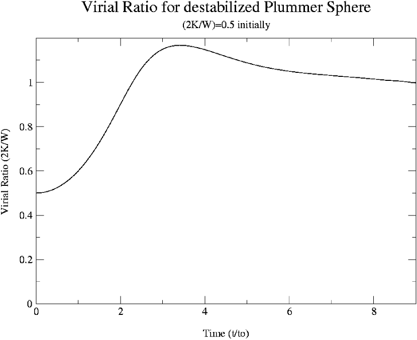
Figure 1: Evolution with time of virial ratio for $n=5$ polytrope with initial virial ratio 0.5. The virial ratio peaks and approaches unity, with the system essentially at virial equilibrium within eight characteristic times.

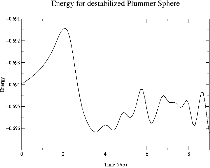
Figure 2: Evolution with time of energy for $n=5$ polytrope with initial virial ratio 0.5. Over nine characteristic times, the energy is conserved to within 0.5%.

Starting from $\left|2K/W\right|=0.5$, we can see that the virial ratio peaks above unity, then decreases toward that value. We note the absence of vigorous oscillations in the virial ratio about the equilibrium value.

At first glance the absence of oscillations may appear to contradict the results of David & Theuns (1989), who observed long-lived radial pulsations in $N$-body collapse simulations of homogeneous spheres. However the results shown in Fig. (1) confirm those seen by Rasio, Shapiro & Teukolsky (1989) (their fig. 2). Those authors conclude that the adaptive integration method produces results which approximate an $N$-body integration as $N\to\infty$, and so suppresses the virial oscillations which likely result from finite-number effects.

We have tested this supression using the N-body treecode to calculate the virial ratio for the same case as in Fig.  (2) using various particle numbers with the tree code that is used below. The direct integration calculation is superimposed. We see clearly that the increasing number of particles reduces the amplitude of the oscillation. Only very weak and smooth oscillations remain in the largest number used. The direct integration accurately reproduces this large $N$ behaviour as far as the calculation could be continued. It is likely that subsequent behaviour of the direct integration would show even weaker oscillation, but we are unable to demonstrate this because of the time requirements of the CBE code.

A subsequent test was performed using the N-body treecode by repeatedly evolving a destabilized galactic halo (as decribed in section 2.5) with initial virial ratio of $0.5$ with different numbers of particles. We are able to run this code over a much larger number of relaxation times than is the case for the CBE integration. These results are reported in Fig. (3) where we see in fact that the virial oscillation amplitude decreases as the particle number is increased.

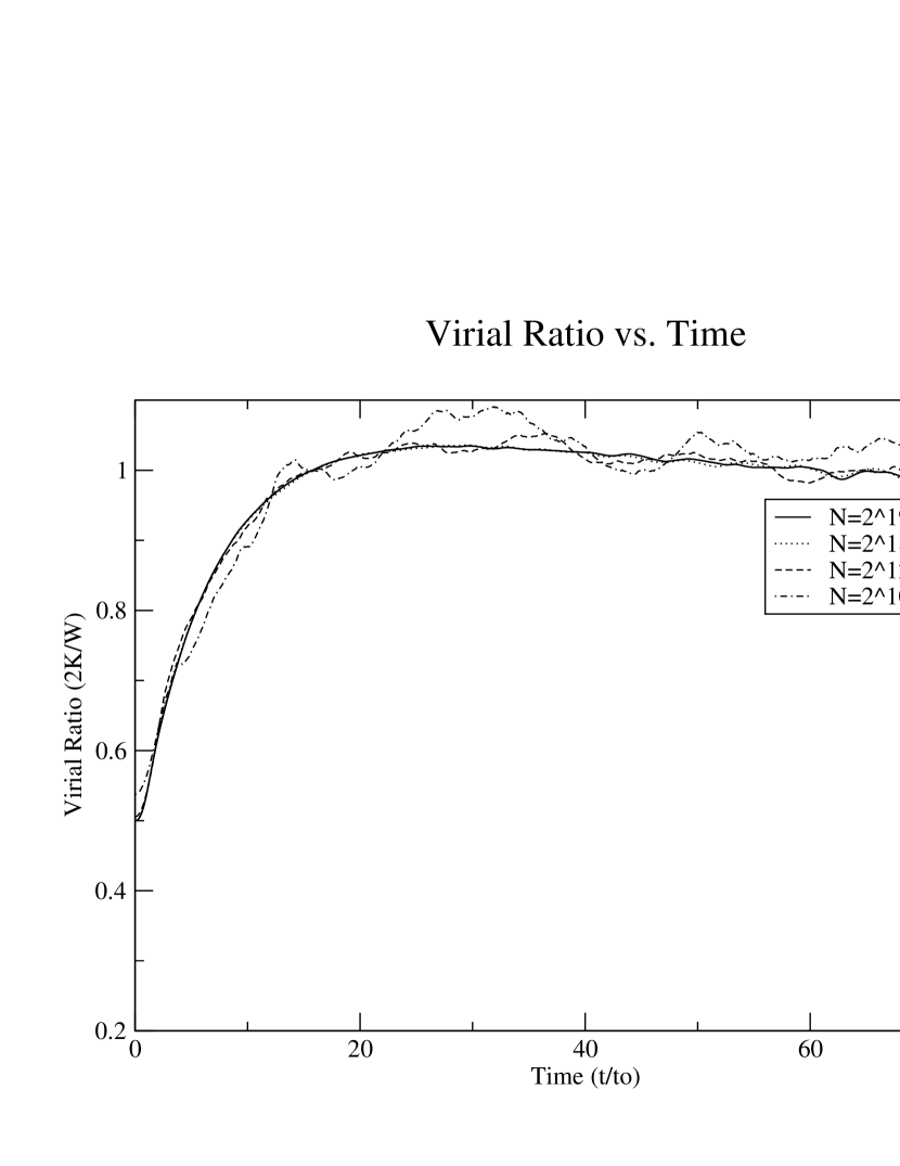
Figure 3: Evolution with time of virial ratio for a self-gravitating system of particles with initial virial ratio 0.5. Oscillations and numerical artifacts are suppressed as the number of particles is increased. This supports the assertion that the direct integration method does, in fact, allow us to approach the continuum limit.

We conclude that not only are any virial oscillations appearing in this type of simulation likely due to finite number effects but that in addition the results of this section are consistent with those obtained through traditional $N$-body methods in a significantly smaller number of relaxation times.

Having established empirically that the virial oscillations are most visible with a smaller number of particles in the system, and that the direct integration approaches the infinite particle limit, we must nevertheless be careful not to dismiss the oscillations as merely errors. There could be finite number effects that are physical and indeed those observed do exceed the $1/\sqrt{N}$ fluctuation noise (we are indebted to a referee for this remark). It is possible that we are seeing the wave-particle aspect of violent relaxation (Funato, Makino and Ebisuzaki 1992a,b) best in the small systems. For in these systems the short wavelength time disturbances will be suppressed due to lack of numerical resolution, leaving only the more global oscillations and relaxation. And in support of this idea we see that the oscillations in Fig.   (4) have periods of several crossing times in the most pronounced case.

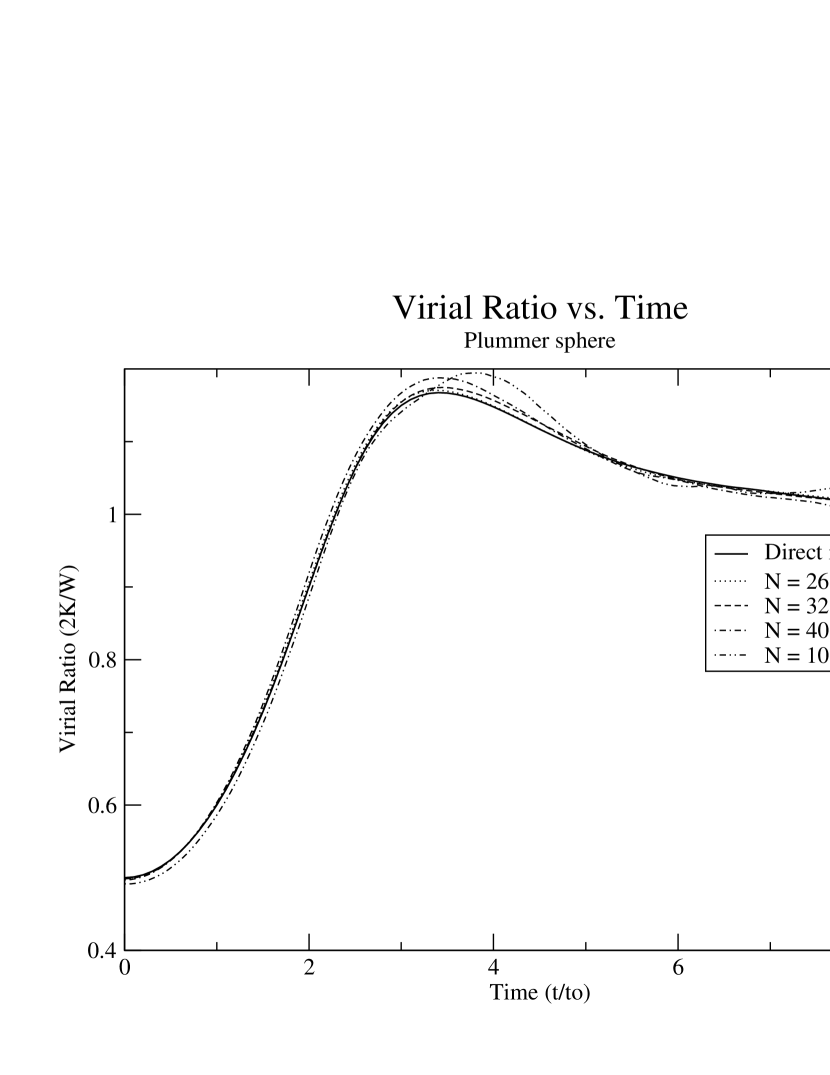
Figure 4: In this figure we show the virial ratio for the n=5 polytrope (Plummer Sphere) calculated using the tree code for a variety of particle numbers. The direct integration calculation is superimposed. The finite number effects are clearly visible, and only a very weak smooth oscillation remains with the largest number of particles.

As the number of particles increases, the short wavelengths should be progressively filled in and the relaxation will become more complete on all scales. This is probably the import of the observed stabilization of the virial ratio with increasing $N$ and in the direct integration limit.

Thus rather than being considered as errors the oscillations in small $N$ systems should be seen as providing a means of studying the actual development of the collisionless relaxation. It is likely that the onset of the phase mixing instability that we report is only evident with sufficiently large $N$ for example. However this is not the main interest of the present work, wherein we choose rather to study the evolution of the DF.

Returning to Fig. (1) which should represent the large $N$ limit as argued above, we conclude that after approximately eight characteristic times the cloud is almost fully virialized ($2K/W=1.01$). Using values for a dark matter halo obtained through observations of satellites of the Milky Way (M${}_{halo}\sim 1.3\times 10^{12}$M_⊙, R${}_{halo}\sim\;160$ kpc) (Little & Tremaine 1987; Arnold 1992) to scale our results, one finds that the system has almost fully relaxed in approximately $6.6$ Gyr.

The density profile of the virialized cloud (Fig. (5)), shows that the central core has contracted and the density has increased with respect to its initial value.

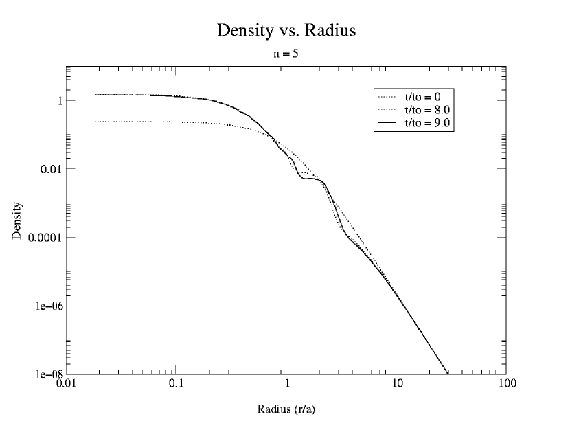
Figure 5: Evolution with time of density for $n=5$ polytrope with initial virial ratio 0.5. Density waves are clearly seen propagating outward.

There are also what appear to be density ‘waves’ propagating into the outer regions. As the system relaxes, particles initially close to the center are pulled into the potential well more tightly, causing the central density enhancement. Particles from farther out pass close to the center of the distribution, gaining kinetic energy as they collapse. They are then flung back to the outer regions and pass through incoming particles. Finally they are turned around by the increasing central attraction, which produces a ‘winding’ of the DF. Fig. (6) shows how the collapse proceeds in phase-space for two different collapse calculations.

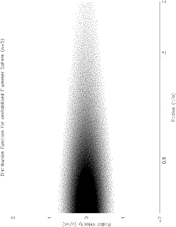
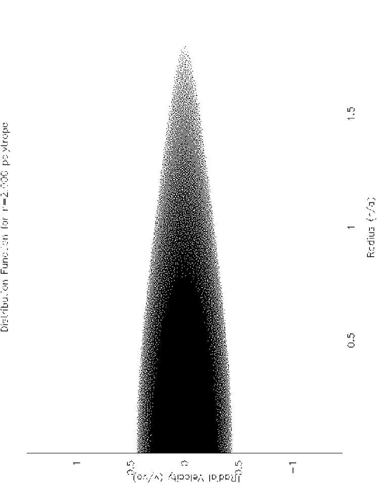
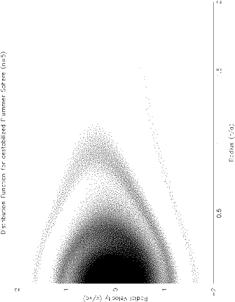
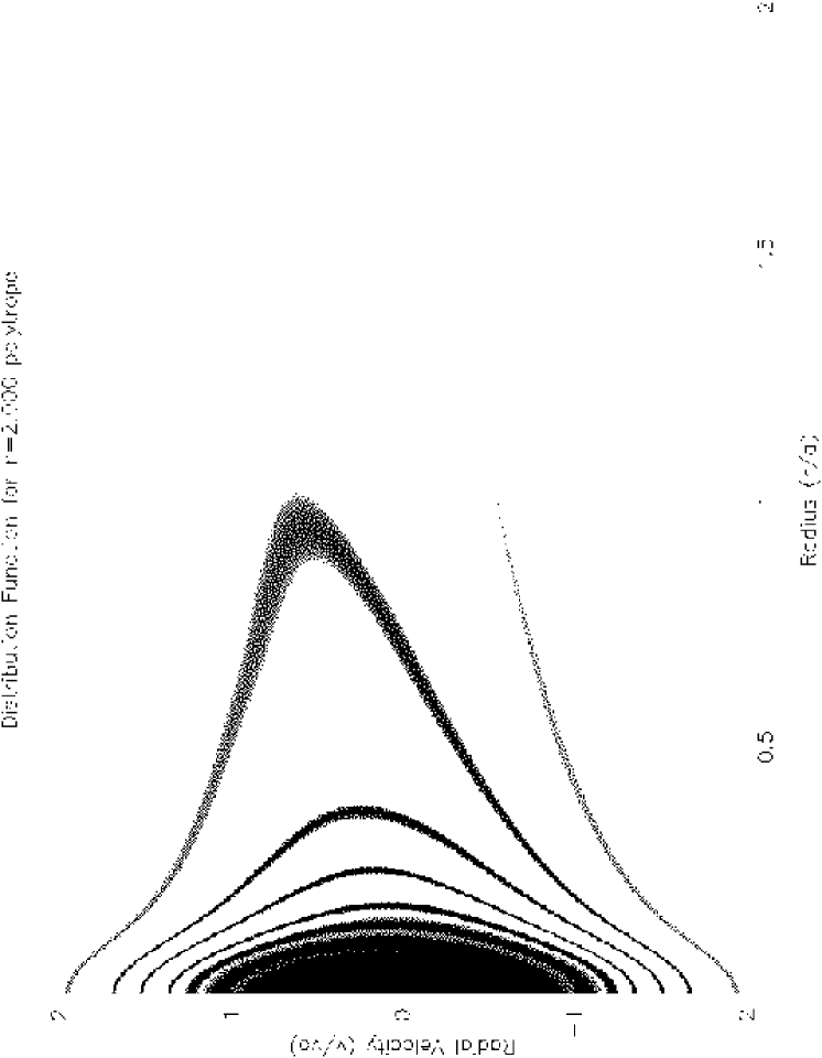
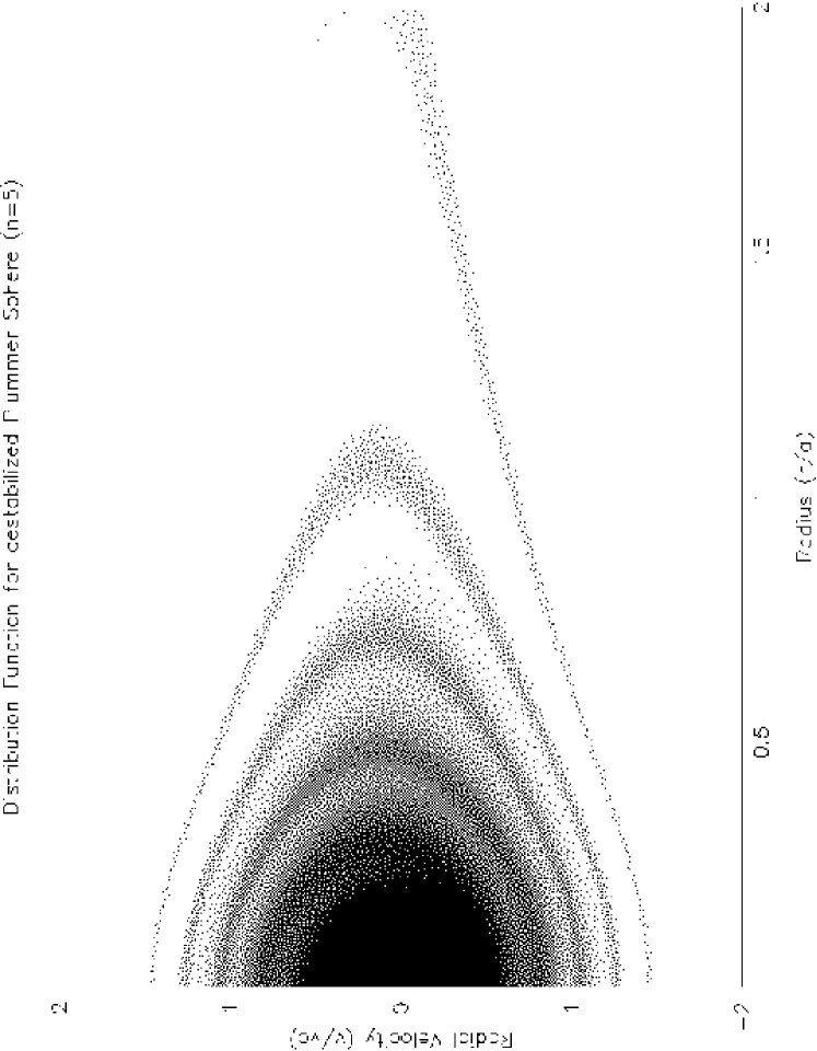
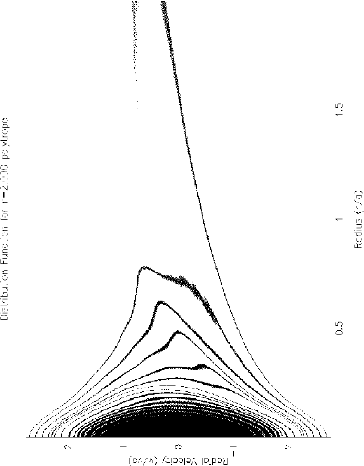
Figure 6: $j=0$ slices of phase space portrait for $n=5$ (left column) and $n=2$ (right column) polytrope with initial virial ratio 0.5 and 0.1 respectively. Times shown are (from top) $t/t_{o}=0.0,\,4.0,\,8.0$.

The growth of the phase-mixing spiral ‘stream’ in phase space is thus perceived as a train of outward propagating density ‘waves’ in physical space. However they are really best understood in phase space. As the system is cooled, the peaks become much sharper, eventually approaching the ‘smoothed infinite peaks’ observed by Fillmore & Goldreich (1984) in their particle simulations.

In addition to the $\alpha^{2}=2$ case considered above, simulations were performed using very cold initial conditions ($\alpha^{2}=20$). Qualitatively, many of the features seen above were also present in this case (central density enhancement, density ‘waves’ due to multiple streaming). One new feature, however, was observed in the phase-space portrait. An instability in the phase streams was seen during the collapse (see Fig. (6, bottom right panel) for an example of the same instability as seen in the $n=2$, $\alpha^{2}=10$ case). This instability does not appear in warmer collapse simulations (Fig. (6), bottom left panel) when the ‘smoothing’ pre-exists.

This instability appears quite similar to one described by Henriksen & Widrow (1997). In their shell-code simulations, the radial instability was observed to blur the windings of the DF in phase space and to produce a smoother, more relaxed DF (see their fig. 1). Their interpretation is consistent with our result in which the central regions, still showing distinct streams after one characteristic time, have at the resolution level of this simulation blended into a more continuous DF after four characteristic times.

It is conjectured that this instability is one of the mechanisms by which a cold system can approach the smooth maximum-entropy state. The observed instability spreads the infalling phase streams out and allows an approach to a finer grained equilibrium. The initially warmer simulations are free of the instability due to the initial spread in velocities. Reducing the discreteness of the velocity streams appears to reduce the strength of the instability and the initial DF is already sufficiently “smeared” in velocity space that a smooth final state does not require the destabilizing of the phase streams. The wave-particle aspect of ‘violent relaxation’ must still operate however.

It was suggested in Henriksen & Le Delliou (2002), that relaxation may be said to be complete when the finer grained (but still statistically valid) DF and less finely grained DF coincide. This is a useful notion but clearly it is bounded at the two ends of the resolution scale. If the resolution is such that an individual particle may be followed then clearly the DF description is not useful. On the other hand a resolution which just resolves the system would provide no structural information. There is then an optimum smoothing range over which to test the invariance of the relaxed DF. Practically, in our direct integration results, we simply coarse grain until until the DF is smoothly varying. This requires typically a $20$% smoothing in velocity space. Our N-body calculations are presented unsmoothed.

4.1.3 Velocity distribution

The extent (completeness) of any ultimate Gaussian will be limited by the finite mass and radius, since a complete Gaussian profile (i.e. extending to infinite positive and negative velocities) would correspondingly require infinite mass and radius. So, when we speak of a Gaussian velocity distribution, it is with the implicit understanding that it must be lowered in such a manner as to be truncated at some finite velocity (since, of course, $f$ can never be negative).

Lowering a Gaussian was considered by King (1966), who determined that the cutoff and the method of lowering the curve have very little effect on the central regions, with deviation in the density profile appearing only near the spatial limit of the distribution. A lowered Gaussian will have the effect of including only those particles with negative energy (bound particles). The method of modifying the DF to include only those stars with negative energy has been discussed by King (1966), Binney & Tremaine (1987), and Kuijken & Dubinski (1994). While it is true that a lowered Gaussian is not strictly a Gaussian (as it does not lie within an infinite domain), up to the point where $f=0$ the velocity distribution should have a Gaussian shape consistent with predictions (Nakamura,2000).

As the destabilized polytrope collapses, the finest-grained DF spirals in phase space, leading to a series of peaks in the velocity distribution (Fig. (7)).

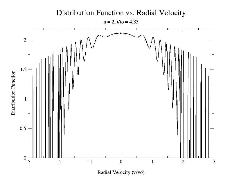
Figure 7: Profile of DF vs. radial velocity for $n=2$ polytrope with initial virial ratio 0.1 after 4.35 characteristic times. This profile is taken at $r=0$.

By smoothing the velocity distribution with a moving window average, we are able to determine a coarser grained DF. We find that the smoothed DF is indeed Gaussian (Fig.  (8)) up to the edge of the distribution in velocity space. The figures are shown for the centres of the polytropes.

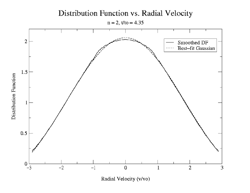
Figure 8: Profile of DF vs. radial velocity for $n=2$ polytrope with initial virial ratio 0.1 after 4.35 characteristic times, smoothed with a window of 20% of the total width. Also shown is the best-fit Gaussian ($DF=2.606\;exp\!\left(-0.15v_{r}^{2}\right)-0.549$). This profile is taken at $r=0$.

The window function used in the smoothing was a simple top-hat averaging, centered on the point under consideration. A Gaussian distribution has not been imposed anywhere in the calculation process, and the Gaussian shape of the smoothed distribution appears to be a result of the relaxation process rather than an artifact of the smoothing. The width of the window was adjusted to smooth over all the peaks in the finest-grained DF, while still maintaining a significant ‘fine-grained’ signal. Choosing too small a window (too high a resolution) does not sufficiently smooth the spikes (leaving non-equilibrium features in the profile), while oversmoothing the distribution with too large a window causes a suppression of the signal. The signal is completely suppressed in the limit of the coarsest-grained smoothing that would simply produce a completely flat DF. The top-hat width used was always the same fraction of the total width of the velocity distribution in the various figures.

It is clear that at the full resolution of this simulation the system has not relaxed microscopically because the phase space ‘spiral’ is only beginning to be subject to the phase mixing instability. We would expect that in time the smoothed or coarse-grained DF will become valid on finer and finer scales. The calculation became very time consuming at this point and so we decided to test the DF over longer time scales with an N-body tree code. There (see below) one does see the phase space structure becoming smooth at a fixed resolution.

A velocity distribution from an earlier time (before the central region has approached its relaxed state) was smoothed with the same window as Fig. (8), and is clearly not Gaussian (Fig. (9)).

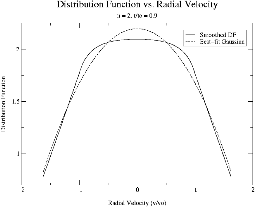
Figure 9: Profile of DF vs. radial velocity for $n=2$ polytrope with initial virial ratio 0.1 after 0.9 characteristic times, smoothed with a window of 20% of the total width. Also shown is the best-fit Gaussian. It is clear that it this early stage in the relaxation process the DF has not yet established a Gaussian velocity profile. This profile is taken at $r=0$.

This supports the idea that as time passes the distribution becomes more nearly Gaussian, and that the Gaussian signals seen are not simply artifacts of the smoothing. Fig. (10) illustrates the effect for the $n=4$ case. This demonstrates that the evolution to Gaussianity does not rely on a particular value of $n$ to take place, and should occur for a general spherical collapse.

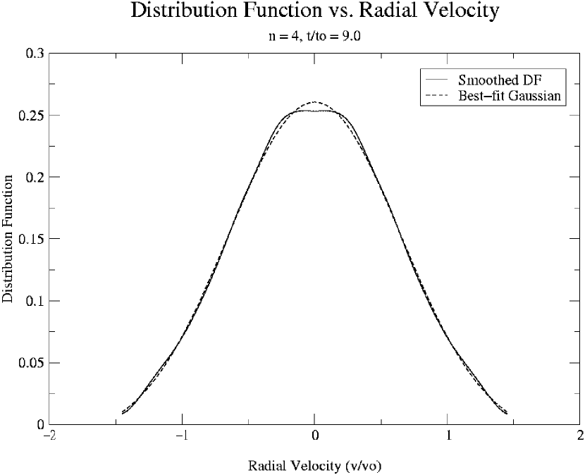
Figure 10: Profile of DF vs. radial velocity for $n=4$ polytrope with initial virial ratio 0.667 after 9.0 characteristic times, smoothed with a window of 20% of the total width. Also shown is the best-fit Gaussian. This profile is taken at $r=0$.

The smoothing of the DF by a moving window average is an approximation to a coarse-graining of the system. In Henriksen & Le Delliou (2002), a coarse graining scheme is proposed which involves a nonuniform rescaling of the phase space. This scheme produces a series representation of the DF which is interpreted as progressively finer graining at higher orders. They discover that the best behaved coarse graining expansion is that which produces a Gaussian velocity distribution in the inner (relaxed) region, in agreement with the statistical arguments of Lynden-Bell (1967) and Nakamura (2000). Our current investigation confirms both the Gaussian inner distribution, and their supposition that the deviation from the relaxed state increases with radius.

4.2 Collapsing Halo Results

The input parameters for the KD code and the resulting dimensionless halo properties are summarized in Tables (1)–(2).

Table 1: Kuijken & Dubinski halo parameters (Model 1)

$\Psi_{o}$	= -8.0			Total Mass	: 42.313$M_{o}$
$v_{o}$	= $\sqrt{2}$			Tidal Radius	: 87.58$R_{o}$
$q$	= 1			King Radius	: 5.211$R_{o}$
$(r_{c}/r_{k})^{2}$	= 1
$R_{a}$	= 1

Table 2: Kuijken & Dubinski halo parameters (Model 2)

$\Psi_{o}$	= -8.0			Total Mass	: 4.344$M_{o}$
$v_{o}$	= $\sqrt{2}$			Tidal Radius	: 8.98$R_{o}$
$q$	= 1			King Radius	: 0.5212$R_{o}$
$(r_{c}/r_{k})^{2}$	= 1
$R_{a}$	= 0.1

In order to get physically meaningful quantities from the scaled variables, we used the same dark matter halo parameters as above (M${}_{halo}\sim 1.3\times 10^{12}$M_⊙, R${}_{halo}\sim\;160$ kpc) (Little & Tremaine 1987; Arnold 1992). These values lead to the scalings presented in Tables (3)–(4).

Table 3: Kuijken & Dubinski halo physical scalings (Model 1)

$M_{o}$	= 3.0723$\times 10^{10}$ M⊙
$R_{o}$	= 1.827 kpc
$t_{o}$ = $\sqrt{R_{o}^{3}/GM_{o}}$	= 6.6425$\times 10^{6}$ years
$v_{o}$ = $\sqrt{GM_{o}/R_{o}}$	= 268.9 km s-1
$\sigma_{o}$ = $v_{o}$/$\sqrt{2}$	= 190.17 km s-1
$T_{\mbox{core}}$ = $2\pi r_{k}/\sqrt{3}\sigma_{o}$	= 18.90$t_{o}$
$T_{\mbox{cross}}$ = $2R_{t}/\sigma_{o}$	= 175.16$t_{o}$

Table 4: Kuijken & Dubinski halo physical scalings (Model 2)

$M_{o}$	= 2.9926$\times 10^{11}$ M⊙
$R_{o}$	= 17.817 kpc
$t_{o}$ = $\sqrt{R_{o}^{3}/GM_{o}}$	= 64.79$\times 10^{6}$ years
$v_{o}$ = $\sqrt{GM_{o}/R_{o}}$	= 268.74 km s-1
$\sigma_{o}$ = $v_{o}$/$\sqrt{2}$	= 190.03 km s-1
$T_{\mbox{core}}$ = $2\pi r_{k}/\sqrt{3}\sigma_{o}$	= 2.67$t_{o}$
$T_{\mbox{cross}}$ = $2R_{t}/\sigma_{o}$	= 25.41$t_{o}$

The N-body haloes produced by the KD94 code were destabilized by reducing the velocities by a constant factor just as in the polytropic collapse considered above. This reduced the thermal support and facilitated the collapse of the halo. In the first case, we used a velocity reduction factor of $\alpha^{2}=2$ applied to a Model 1 halo. This is a fairly warm collapse and, as such, we do not expect to see significant growth of the Henriksen & Widrow (1997) phase mixing instability.

The relaxation of the Model 1 halo proceeds in much the same manner as for the spherical polytropes calculated with the CBE code above. As the collapse progresses, the velocity distribution spreads in order to provide the necessary thermal support to stabilize the configuration. The peaks shown in Fig. (11) were similar to those seen in Fig. (7) and were evident in the collapse at various radii.

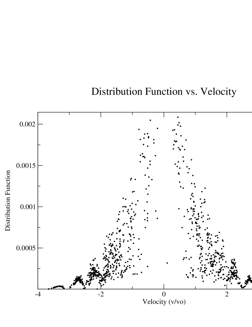
Figure 11: Profile of DF vs. radial velocity for a galactic halo (Model 1) with initial virial ratio 0.5, prior to relaxation of the halo ($t/t_{o}=20$). This slice is taken at a radial bin of width 0.05, centered at 2.0. Peaks in the velocity distribution corresponding to distinct phase streams are apparent in the wings of the distribution.

The finite resolution coming from the discrete nature of the N-body simulation causes the peaks in the velocity distribution to become indistinct and blur in time into a more continuous distribution.

Fig. (12) shows the increasing velocity width in the approach to the equilibrium state at $r=0.9$. Fig. (13) shows the velocity distribution closer to the center of the halo ($r=0.15$, as compared to $r=0.9$). At this time, the velocity distribution in this central region has already evolved to a near-Gaussian form (Fig. (13)), but the distribution farther out still shows evidence of non-Gaussianity in the form of noticeable streams in the wings of the distribution (Fig. (11) – (12)). In time the velocity distributions at larger radii will also evolve to near-Gaussian form as they spread to provide ‘thermal’ support.

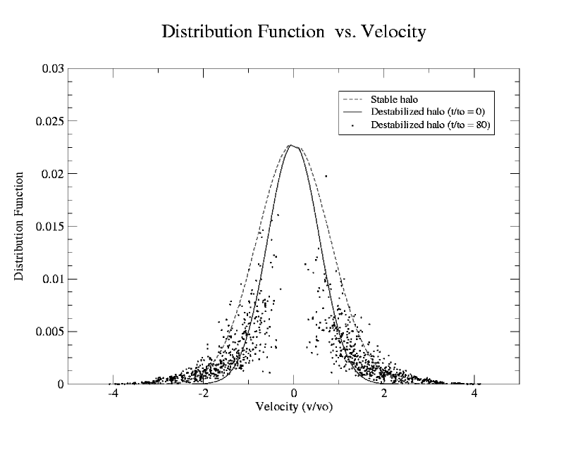
Figure 12: Profile of DF vs. radial velocity for a galactic halo (Model 1) with initial virial ratio 0.5. This slice is taken at a radial bin of width 0.05, centered at 0.95.

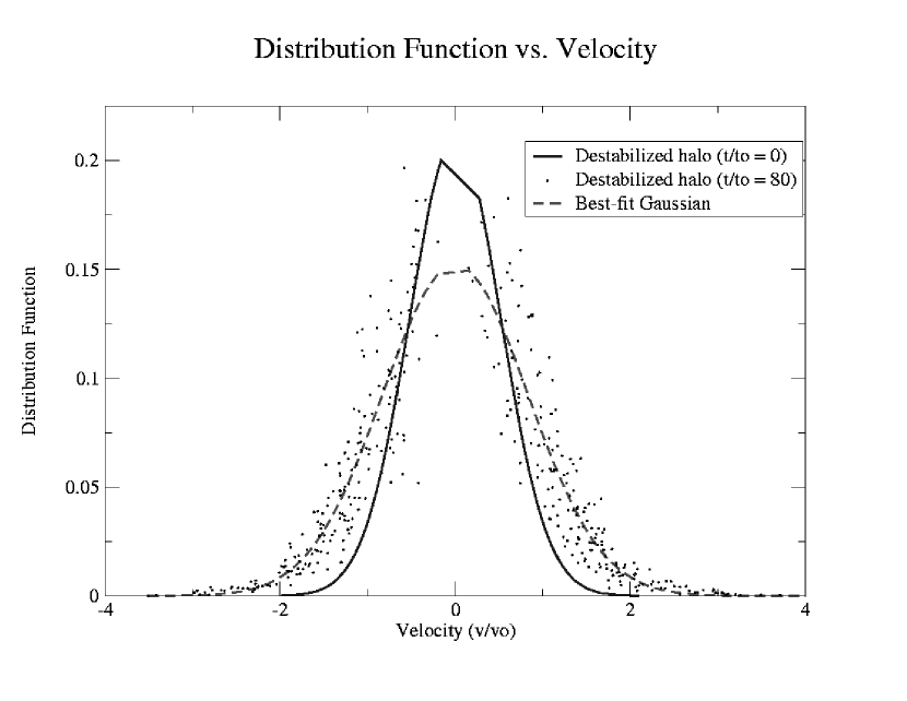
Figure 13: Profile of DF vs. radial velocity for a galactic halo (Model 1) with initial virial ratio 0.5. This slice is taken at a radial bin of width 0.05, centered at 0.15. The flattening at the peak of the initial and stable halo distributions is simply a result of having too few points with near-zero velocity to completely define the curve.

For the Model 2 halo, an initial virial ratio of 0.25 was chosen. This value is on the edge of the ‘cool’ domain where we expect the Henriksen & Widrow (1997) instability to play a rôle in relaxation.

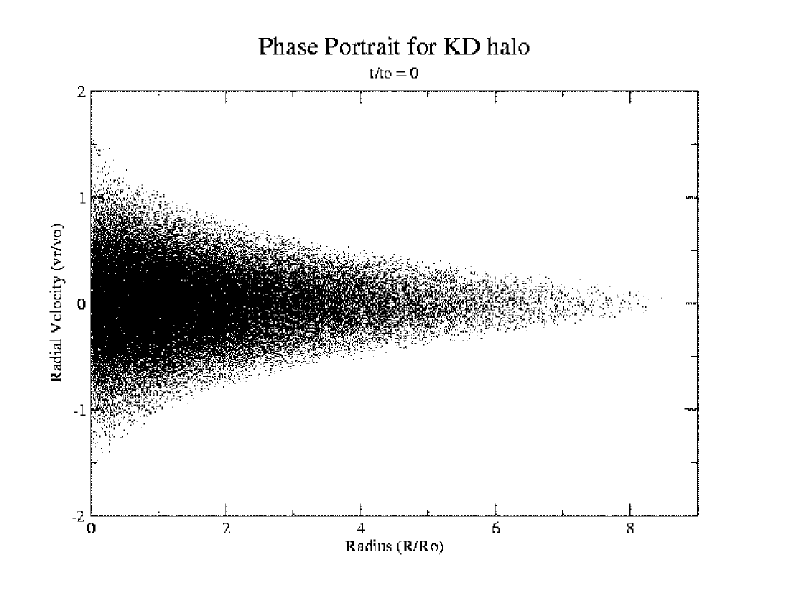
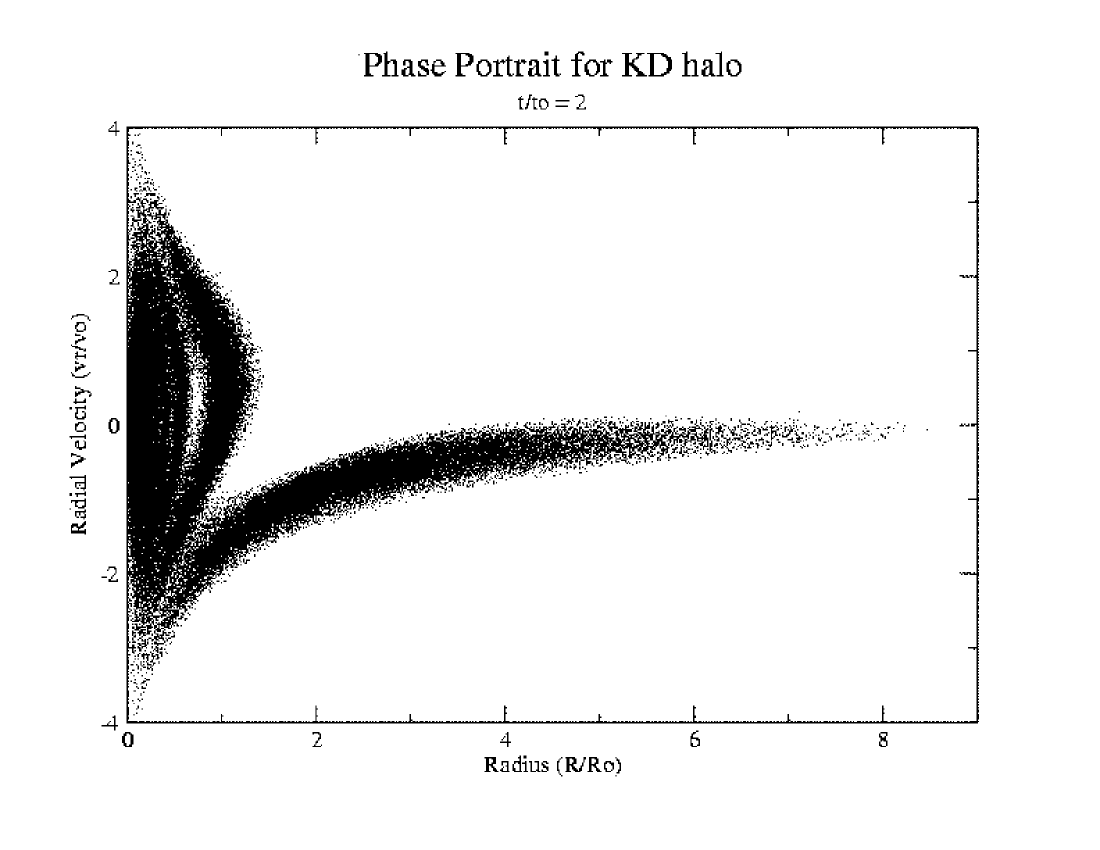
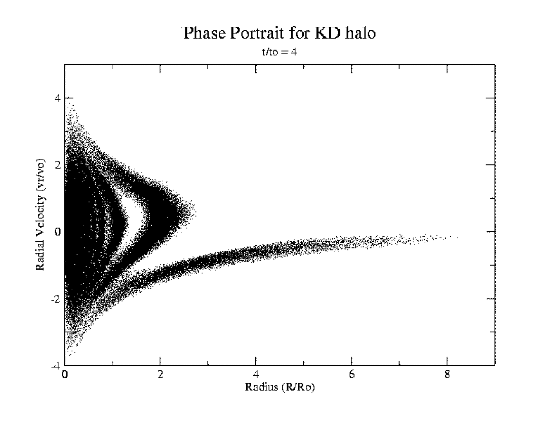
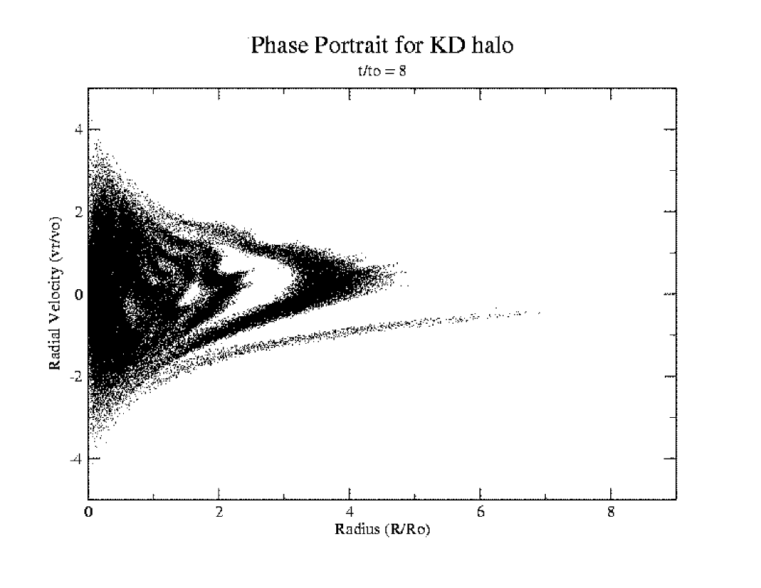
Figure 14: ($r$, $v_{r}$) projection of a collapsing KD halo (Model 2) with $\alpha^{2}=4$. Time increases from left to right, top to bottom. Times shown are $t/t_{o}$ = 0, 2, 4, 8.

As the collapse proceeds, we find very similar results to those found with the CBE calculation. The DF phase mixes in the projected ($r$, $v_{r}$) phase-space (Fig. (14)) – also observed in configuration space as a set of outward propagating density ‘waves’ (Fig. (15))

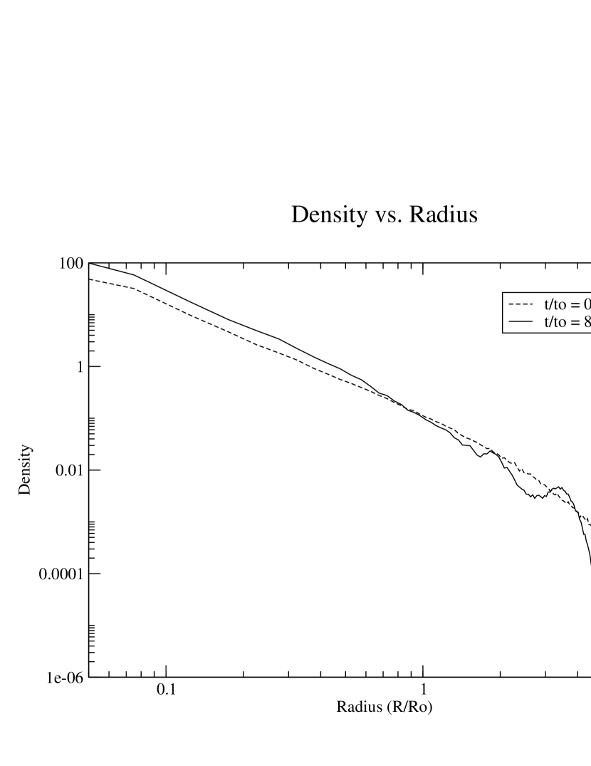
Figure 15: Evolution with time of density for a galactic halo (Model 2) with initial virial ratio 0.25. Density waves are clearly seen propagating outward. The power-law region of the final state goes as $r^{-3}$.

and again in the velocity distribution as a set of peaks (seen dominating the velocity distribution in Fig. (16)),

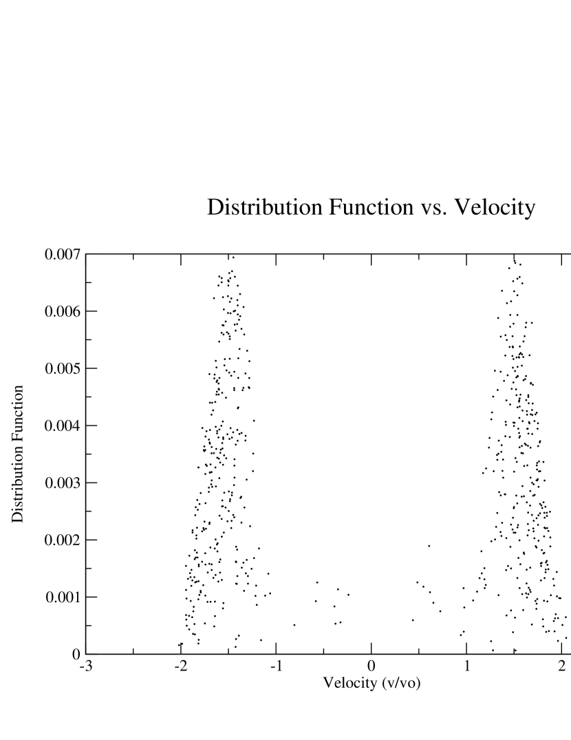
Figure 16: Profile of DF vs. velocity for a galactic halo (Model 2) with initial virial ratio 0.25. This slice is taken at a radial bin of width 0.05, centered at 0.75. The velocity distribution is dominated by two large peaks (velocity streams).

which spread and become less distinct in time (Fig. (17)).

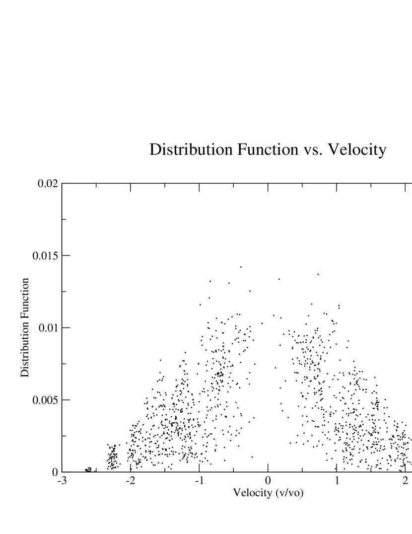
Figure 17: Profile of DF vs. velocity for a galactic halo (Model 2) with initial virial ratio 0.25. This slice is taken at a radial bin of width 0.05, centered at 0.75. The velocity distribution is in the process of relaxing to Gaussianity, and the peaks in the wings of the distribution which dominated the velocity distribution in Fig. (16) have become much less prominent due to the onset of the Henriksen & Widrow hw97 instability.

The onset of the phase mixing instability can be seen in the bottom right panel of Fig. (14). We note that the central regions have already become close to Gaussian (Fig. (18)).

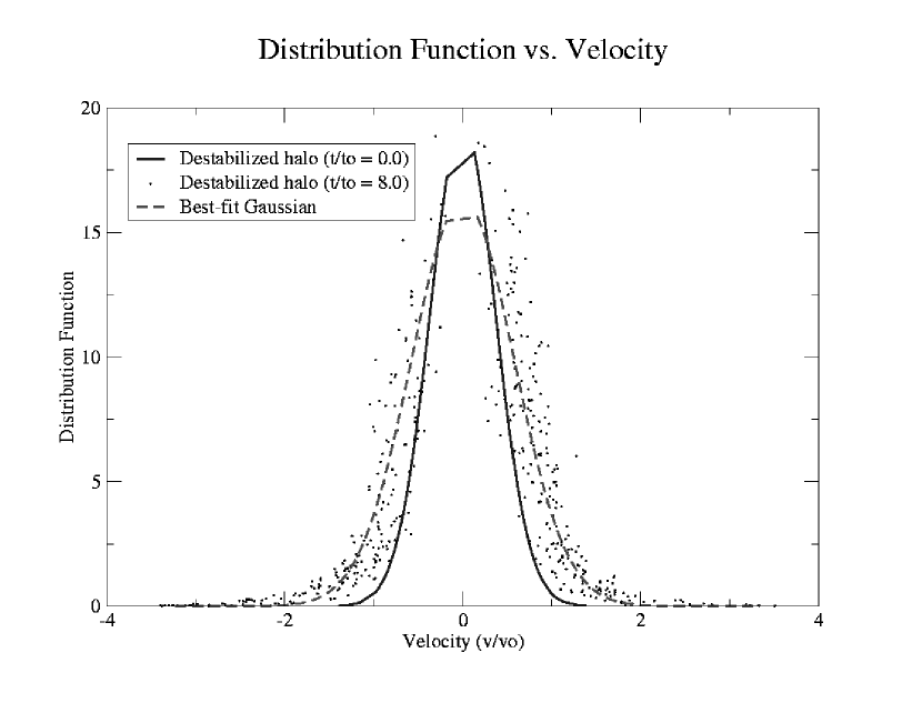
Figure 18: Profile of DF vs. velocity for a galactic halo (Model 2) with initial virial ratio 0.25. This slice is taken at a radial bin of width 0.05, centered at 0.025. The velocity distribution has almost reached a relaxed Gaussian state.

The width of the distribution has once again increased to provide the thermal support required to halt collapse.

The DF–Energy correlation is plotted in Fig. (19).

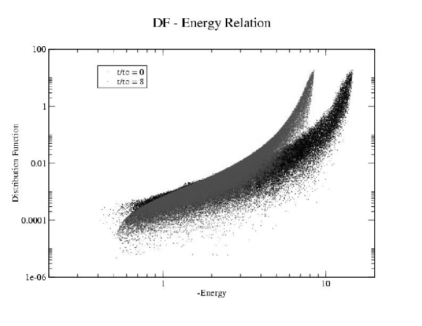
Figure 19: Distribution Function – Energy relationship for a KD halo (Model 2) with an initial virial ratio of 0.25. For this halo, the rough shape of the relation is maintained, with the most negative energy particles becoming more tightly bound as collapse progresses.

As the halo relaxes to its new equilibrium, we can see that the overall shape of the curve is maintained, although the larger phase space density (higher $f$) particles (corresponding to those that initially have more negative energy) becoming even more tightly bound as time passes. Funato, Makino & Ebisuzaki (1992a) also observed this energy segregation through violent relaxation, but they interpreted this as meaning that the Gaussian distribution would not be realized in practice. Our results demonstrate that although violent relaxation does segregate energies, a Gaussian velocity distribution can nevertheless result from the collapse.

The fact that the shape of the $f(E)$ relation is maintained suggests that the particles retain some memory of their initial state throughout the relaxation process. This is consistent with the results of van Albada (1982), who also observed correlation between initial and final energies in violently-relaxing particles as did Henriksen and Widrow (1999). This ‘moderate’ Violent relaxation is nevertheless a process which acts over a much shorter timescale than two-body relaxation in the systems studied. Thus we conclude that a collisionless collapse needs only a moderate dispersion in energy at each position,in order to produce a Gaussian velocity distribution.

The behaviour of the virial ratio is shown for a typical case in Fig. (3). We see not only the finite number effects referred to previously but the trend toward an ultimate virial ratio different from unity. This is a numerical effect which results from calculating the potential energy using the exact summation over the $1/r$ potentials of a set of pointlike particles in a system which evolves under a softened force. This effect is well known and is due to the slight inconsistency of evolving the system under a softened gravitational force, while calculating the potential energy from the unsoftened potential.

4.3 Colliding Halo Results

In this section spherical symmetry is explicitly broken by modelling the merging of two centrally cusped galactic haloes. We performed six merger simulations. All six consisted of the merging of two identical stable galaxy models (KD Model 2 – see Tables 2 & 4 for halo parameters and physical scalings respectively). The collision parameters are summarized in Table 5.

In the first simulation, the two galaxies were placed with their centers separated by a distance $54R_{o}=0.962$ Mpc, with a relative approach velocity of $1.4v_{o}=376.24$km s^-1. This approach velocity is approximately half of what it would be if the galaxies had come from infinity with zero initial velocity. In the second simulation, the galaxies were initially at rest with respect to one another with their centers separated by $24R_{o}=427.6$ kpc. The third simulation had the galaxies starting from a separation of almost $2.5$ Mpc, with initial velocities of $40.3$km s^-1. The initial conditions of this third simulation are such that the difference in the interaction (tidal) gravitational potential across each galaxy is very small. This was intended to minimize the initial disequilibrium of the haloes. The fourth simulation began with the galaxies already overlapping and with zero relative velocity (more like a fragmentation). The centers are separated by $4.5R_{o}=80$ kpc (which places the edges of the King radii approximately $4.5R_{o}$ apart). The fifth and sixth “collision” (again more like fragmentation) simulations had the cores of the haloes initially overlapping, and zero relative velocity. Simulation 5 begins with zero distance between the centers of the haloes, and simulation 6 begins with the centers separated by $1R_{o}=17.8$ kpc. The initial distance between the haloes in simulation 6 places the King radii of the haloes in tangential contact.

The virial ratio and total energy are both well conserved in these simulations, with the virial ratio approaching unity (but see comment in the previous section) shortly after the merging and the energy remaining within $1\%$ of the initial value throughout the lifetime of the simulation. The simulations were allowed to run for almost 12 Gyr (simulation 1), over 17 Gyr (simulation 2), over 50 Gyr (simulation 3), 13 Gyr (simulation 4), and 1.3 Gyr (simulations 5 & 6).

The final density profile of simulation 2 is typical of that found in the first three merger simulations, and is shown in Fig. (20).

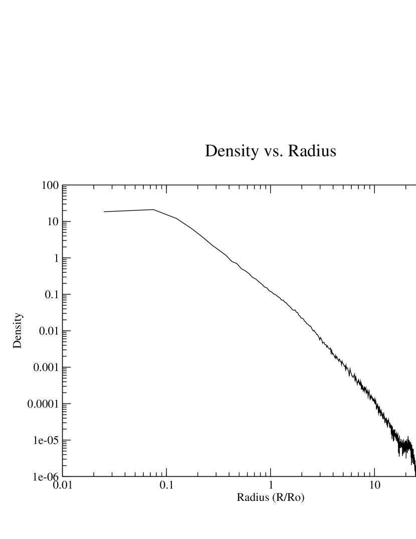
Figure 20: Final density profile for a pair of colliding galactic haloes (Simulation 2). This figure is taken at a time $t=10.1$ Gyr after the initial contact. The power-law region of the final state goes as $r^{-3}$ between the edge of the core region and the first outgoing density peak at $\sim 25R_{o}$.

It is seen to exhibit a flat central region, with a power-law envelope which falls off as $r^{-3}$. This observation is consistent with the results of White white78 white79 , who found the same behaviour in an extensive examination of elliptical galaxy mergers.

Simulations 4 – 6 have final density profiles which are different from $r^{-3}$ and, in fact, show two different power-law regions in addition to the flat central core. It is interesting that this difference should characterize a kind of re-merging after an earlier fragmentation rather than the violent collisions of the first three mergers. The effect is to suppress the complete transition to $r^{-3}$ – leading to an inner region which is flatter than $r^{-3}$, and an outer region which is steeper. The final density profile of simulation 4 is shown in Fig. (21).

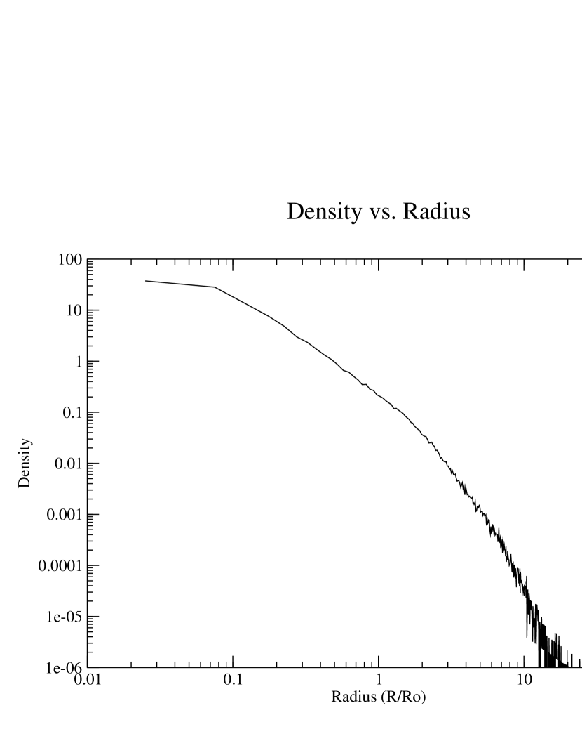
Figure 21: Final density profile for a pair of initially-overlapping galactic haloes (Simulation 4). This figure is taken after $t=12.9$ Gyr of relaxation. The inner power-law region goes as $r^{-2.2}$, and the outer power-law region goes as $r^{-4.25}$.

This is much like the NFW profile except that there is a flat core.

As all of the haloes relax, the velocity distributions for the collision simulations become centrally peaked at all radii. However, it is not possible to state with any degree of confidence that they are Gaussian (Fig. (22)), at least for simulations 1, 2, and 3.

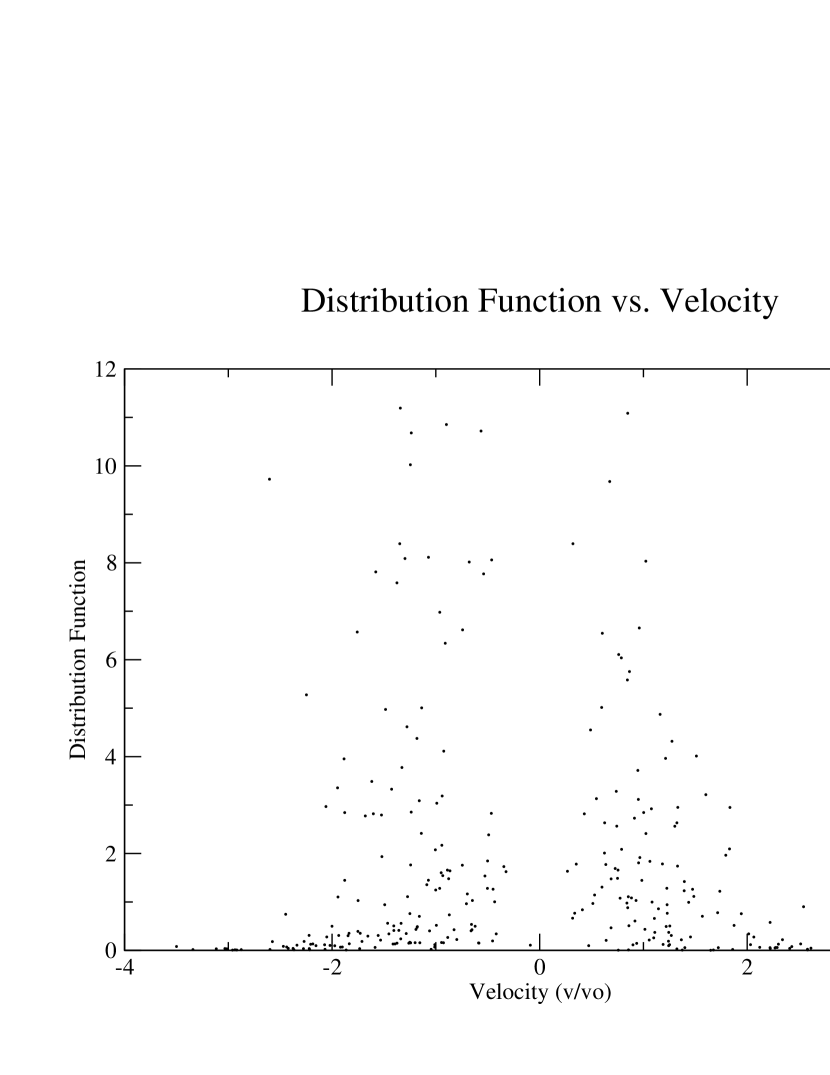
Figure 22: Profile of DF vs. velocity for colliding galactic haloes (Simulation 1). This slice is taken at a radial bin of width 0.05, centered at 0.025. The velocity distribution appears centrally peaked, but is not clearly Gaussian.

Examining the velocity distribution for a small range of $j^{2}$ (rather than for all values of the angular momentum), and angular momentum direction ($\cos{\theta}=j_{z}/\sqrt{j^{2}}$) does not improve the Gaussian fit. An example is given in in Fig. (23).

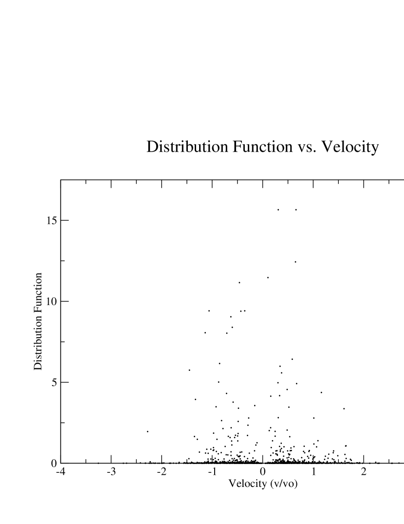
Figure 23: Profile of DF vs. velocity for colliding galactic haloes (Simulation 3). This figure is taken at an angular momentum slice $0\leq j^{2}<0.1$. The velocity distribution appears centrally peaked, but is not clearly Gaussian.

This indicates that the velocity distribution is not segregated by angular momentum with distinct Gaussians appearing in individual $j^{2}$ slices. Rather, we find that the relaxation process is able to distribute angular momentum among the particles, but is unable to produce the predicted distribution.

For simulations 1, 2, 4, 5 & 6, there is a tidal effect previously alluded to that may play a role. Each halo was generated assuming that it was isolated. If that were true, the DF would be a single-valued function of the total energy alone $f=f(E)$ – as in the collapse simulations of section 4.2. When placed in proximity to another halo, the net gravitational potential will no longer be spherically symmetric, and there can, in fact, be a significant potential gradient across the galaxy. This has the effect of changing the total energies of the particles and making $f$ a multi-valued as a function of $E$. Even in the first simulation, when the galaxies are separated by almost 1 Mpc, the change in potential across the galaxy is of order $\sim 5\%$. An energy spread of $5\%$ will give a variation in the DF of $\sim 50\%$ for a weakly bound particle in the KD model 2 halo we considered (taking $E=-0.1$ in the expression for $f$). Even a very tightly bound particle ($E=-10$) will experience a DF spread of $\sim 10\%$. This leads to a very complicated initial DF and this may delay the onset of the Gaussian final state.

However, although the initial multi-valued DF is a major factor affecting the Gaussian signature, it cannot be the only one and ultimately it should not prevent it. Thus simulation 3 was started from initial conditions in which the galaxies were sufficiently far apart that the spread in the Energy – DF relation was small, and yet it also failed to relax to a Gaussian over the lifetime of the simulation (over 20 Gyr after the galaxies’ initial contact).

Funato, Makino & Ebisuzaki (1992a, b) also performed a study of violent relaxation, and found that it proceeds by a combination of wave–particle interaction and phase mixing. In the early stage, the coherent motion of particles causes large-amplitude fluctuations in the potential field. The interaction of the individual particles with this wave can change the energies of the particles significantly in a classic Landau ‘damping’ mode. The waves decay rapidly due to the wave–particle interaction and phase mixing. In the later stages the energy change of the particles is much smaller, since the amplitude of the wave has been significantly reduced. At this point, relaxation proceeds primarily through phase mixing (until the phase-mixing instability becomes important). Funato et al. show that phase mixing in this stage of evolution can be slow in the core, and small oscillations can survive there for a relatively long time (they claim the oscillations can survive for 10 crossing times or more).

We believe that our simulations also display these oscillations, but they also show that they are most visible the more finite the number of particles employed. In the infinite particle limit represented by our direct integration these fluctuations are smoothed to the point of invisibility (Fig. 4) through the addition of very short wavelengths. Nevertheless the persistence of these oscillations tends to support the conclusion of Funato et al.

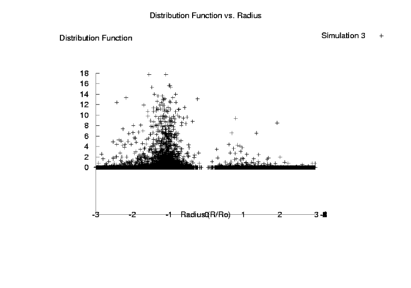
Figure 24: Profile of DF vs. radius for colliding galactic haloes (Simulation 3). This figure clearly shows that the indiviual halo cores have retained some identity within the merger remnant through the relaxation process.

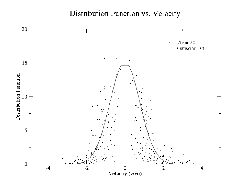
Figure 25: Profile of DF vs. velocity for colliding galactic haloes (Simulation 6). This slice is taken at a radial bin of width 0.05, centered at 0.025. The velocity distribution appears Gaussian, with the curve broadened due to perturbation of the DF–Energy relation of the haloes.

In a merger simulation performed by these same authors (Funato, Makino & Ebisuzaki 1992b), the cores of the initial galaxies remained distinct after the galaxies have merged to one remnant. The two cores oscillate about the center of the remnant. Our $f$($r$) plot for simulation 3 confirms this observation (Fig. (24)). There are evidently two distinct core regions in the final remnant as represented by the double-peaked DF. Funato, Makino & Ebisuzaki (1992a) note that, “violent relaxation disappears within the crossing time scale, no matter whether the system reaches some equilibrium or not.” It appears that in the colliding systems studied here (1,2,3 and 4) the violent relaxation process does not last long enough to produce the Gaussian velocity distribution observed in the isolated collapse simulations. Given our comments above, it is possible that the necessary small scale interactions have not been sufficiently resolved in these calculations. Even a reasonable coarse graining would not however smooth the merger remnant to a convincing Gaussian form.

The initially concentric placement of the haloes in simulation 5 has the effect of simply doubling the potential energy of each particle with no increase in its kinetic energy – essentially generating a single halo with an initial virial ratio of 0.5, similar to those studied in the previous section. Moreover, the effective resolution is increased. It is therfore not surprising that this simulation shows the transition to a Gaussian velocity distribution within a few core orbital periods.

Perhaps our most original result in this section is revealed in simulation 6. The final velocity distribution of the merger remnant in simulation 6 is close to Gaussian in the central region (Fig. (25)). This is true despite the spread in the initial DF–Energy relation so that as has already been remarked, this can not be the dominant factor. Moreover the ‘relaxation’ has occurred in a relatively short time implying that the violent relaxation has been relatively efficient while operating over this short time. It seems then that it more likely to be the case that true collision mergers require too strong a relaxation mechanism for collisionless relaxation to be effective as in Funato, Makino & Ebisuzaki (1992a). Our new observation is essentially that this lack of effective relaxation is correlated with the exterior $r^{-3}$ density profile, while the relaxed systems develop a more nearly NFW type profile outside the core. Moreover, the relaxed systems have formed by a process more similar to fragmentation and subsequent re-merging than to collision of distinct systems.

Table 5: Collision simulation parameters

Label	Initial Separation	Relative Velocity
1	$54R_{o}=0.962$ Mpc	$1.4v_{o}=376.24$km s-1
2	$24R_{o}=427.6$ kpc	0
3	$140R_{o}=2.5$ Mpc	$40.3$km s-1
4	$4.5R_{o}=80$ kpc	0
5	$0$ kpc	0
6	$1R_{o}=17.8$ kpc	0

5 Discussion and Conclusions

We have examined in this paper the relaxation of collisionless systems from non-linearly destabilized initial states toward new equilibrium states. Our work combined with previous work indicates that both violent relaxation (time dependent potential variations and wave-particle interactions) and unstable phase mixing operate. We have also confirmed that these processes are not always sufficient to relax a merging system to a Gaussian DF even at the centre of the system, if the collision is too energetic. This last statement may be resolution dependent since there is a hint that with many more particles the relaxation may be more effective microscopically. However real systems are finite and will have a ‘natural’ resolution with which they should be regarded.

We have demonstrated with two entirely independent computational techniques the approach to a Gaussian velocity distribution of various collapsing isolated systems. In one code (CBE integration method) spherical symmetry is constrained throughout the collapse,while the N-body tree code does not impose any symmetry. We were also able to independently confirm the existence of a radial phase-mixing instability as described by Henriksen & Widrow (1997) using both codes. Our results indicate that an isolated halo will relax toward a Gaussian velocity distribution, with a relaxation timescale of a few Gyr as predicted by some authors (e.g. Nakamura (2000)). This is a fairly robust result since these Gaussian profiles appear in collapsing polytropes of various indices, and in destabilized lowered Evans haloes, when two independent numerical techniques are used. This can happen within a few core orbital periods.

Although several authors (van Albada 1982; Tanekusa 1987; Funato, Makino & Ebisuzaki 1992a, b) have disputed this prediction for various reasons, to our knowledge no one prior to this work has actually examined the velocity-space structure of the end-state to search for the Gaussian signature. By plotting the velocity distributions for different times and radial positions and could actually observe the evolution of the system to the Gaussian form. We confirm that violent relaxation can produce the predicted distribution within a few core orbital periods ((half-mass crossing times in the case of the polytropic collapse models) – exactly the time frame over which violent relaxation is expected to be important.

Although the systems studied here were collisionless (or approximately collisionless, in the case of the particle simulations), they were able to evolve to the predicted Gaussian velocity state. In the case of a cold collapse, an instability was observed which it is believed allows the system to relax by permitting particles to ‘diffuse’ across characteristics in a less than ‘finest-graining’ representation. We expect that the addition of some small collisional interaction will assist the relaxation (as in Tanekusa 1987) also by allowing particles to diffuse across characteristics of the CBE. Such a process would compete with and perhaps suppress the growth of the instability since the phase streams would no longer be so distinct.

We have identified two effects that lead to requiring longer and stronger relaxation than is available by collisionless processes to cause a merger event to forget the initial conditions. One effect is that the halo models were generated assuming they were gravitationally isolated (i.e. no background potential gradient). Thus the DF is a single-valued function of the total energy $E$. In the first two merger simulations, however, the galaxies begin near enough that the gravitational potential across a galaxy changes by $>\sim 5\%$. In this case, the difference in potential across the galaxy is enough to significantly broaden the relation between $f$ and $E$.

The more dominant factor which contributes to the incomplete transition is the limited timescale over which violent relaxation operates, at least with finite ‘resolution’ (a physical effect in finite systems). Sufficient initial asymmetry in the merger for a given number of particles leads to the violent relaxation ending before the memory independent ‘relaxed’ state is reached. That is the bulk oscillations implied by the asymmetry do not degrade to ‘thermal’ motion. We are left then with a system which has only partially proceeded to the maximum entropy state. Subsequent mergers might however restart this process, and if they are gentle enough (or one system is much smaller than the other) ultimately the system may relax. We saw in fact in simulation 6 that systems that are merging in a closely overlapping state with zero relative velocity do relax to the Gaussian form with our resolution. This distinction is also reflected in the final density profiles, wherein the unrelaxed profiles are approximately $r^{-3}$ outside the core, while the relaxed systems have a flat core and what might be described as an exterior NFW profile.

We conclude then by stating that isolated, finite, collisionless systems that form by approximately central collapse should relax to a universal Gaussian form (predicted to be a state of maximum entropy) when appropriately coarse-grained (that is ‘resolved’ or ‘smoothed’). However, those that form through the merging of systems of comparable size will not relax, given the same coarse-graining.

Our present simulations do not start from strict cosmological conditions (although the cold collapses are not so very different) and in particular the initial density profiles have flat cores. Thus we can not comment directly on whether or not the Cold Dark Matter (CDM) heirarchical halo formation theory leads to central cusps or cores. The Gaussian velocity distribution is also compatible with a singular isothermal sphere and the corresponding $r^{-2}$ profile. However one might expect that this isolated solution is not the maximum entropy limit and that in fact the Gaussian distribution corresponds in general to a flat core. Haloes that have not relaxed to the Gaussian state may well show cusp profiles, especially if they have begun in this fashion (unlike our examples). Our results allow us to speculate however that the accretion of a dwarf halo by an unrelaxed massive halo may restart the relaxation process in the large halo. This might lead through a series of such episodic relaxation events to the formation of a flat core. We intend to investigate this speculation in future work.

References

- (1) Arnold R., 1992, MNRAS, 255, 680
- (2) Barnes J., Hut P., 1986, Nature, 324, 446
- (3) Bertschinger E., 1985, ApJS, 58, 39
- (4) Binney J., Tremaine S., 1987, Galactic Dynamics, Princeton University Press, Princeton
- (5) Camm G.L., 1952, MNRAS, 112, 155
- (6) Capelato H.V., de Carvalho R.R., Carlberg R.G., 1995, ApJ, 451, 525
- (7) Chandrasekhar S., 1939, An Introduction to the Study of Stellar Structure, Dover Publications, London
- (8) Cheng C.Z., Knorr G., 1976, J. Comp. Phys., 22, 330
- (9) Dantas C.C., Capelato H.V., de Carvalho R.R., Ribeiro A.L.B., 2002, A&A, 384, 772
- (10) David M., Theuns T., 1989, MNRAS, 240, 957
- (11) Fillmore J.A. and Goldreich P., 1984, ApJ, 281, 1
- (12) Fujiwara T., 1983, PASJ, 35, 547
- (13) Funato Y., Makino J., Ebisuzaki T., 1992a, PASJ, 44, 291
- (14) Funato Y., Makino J., Ebisuzaki T., 1992b, PASJ, 44, 613
- (15) Hénon M., 1973, A&A, 24, 229
- (16) Henriksen R.N., Le Delliou M., 2002, MNRAS, 331, 423
- (17) Henriksen R.N., Widrow L.M., 1995, MNRAS, 276, 679
- (18) Henriksen R.N., Widrow L.M., 1997, Phys. Rev. Lett., 78, 3426
- (19) Henriksen R.N., Widrow L.M., 1999, MNRAS, 302, 321
- (20) Hoffman Y., Shaham J., 1985, ApJ, 297, 16
- (21) Hozumi S., Burkert A., Fujiwara T., 2000, MNRAS, 311, 377
- (22) Hozumi S., Fujiwara T., Kan-ya Y., 1996, PASJ, 48, 503
- (23) Jaynes E.T., 1957, Phys. Rev., 106, 620
- (24) Jaynes E.T., 1957, Phys. Rev., 108, 171
- (25) Kandrup H.E., Mahon M.E., Smith Jr. H., 1994, Phys. Rev. E, 49, 3757
- (26) King I.R., 1966, AJ, 67, 471
- (27) Kippenhahn R., Wiegert A., 1990, Stellar Structure and Evolution, Springer-Verlag, Berlin
- (28) Kuijken K., Dubinski J., 1994, MNRAS, 269, 13
- (29) Kuijken K., Dubinski J., 1995, MNRAS, 277, 1341
- (30) Langmuir I., 1925, Phys. Rev., 26, 585
- (31) Little B., Tremaine S., 1987, ApJ, 320, 493
- (32) Lynden-Bell D., 1967, MNRAS, 36, 101
- (33) Makino J., 1997, ApJ, 478, 58
- (34) Makino J., Ebisuzaki T., 1996, ApJ, 465, 527
- (35) Merritt D., Quinlan G.D., 1998, ApJ, 498, 625
- (36) Nakamura T.K., 2000, ApJ, 531, 739
- (37) Nishida M.T., Yoshizawa M., Watanabe Y., Inagaki S., Kato S., 1981, PASJ, 33, 567
- (38) Quinn T., 2001, in Steves B.A., Maciejewski A.J., eds, Proc. Fifty Fourth Scottish Universities Summer School in Physics, The Restless Universe: Applications of Gravitational N-Body Dynamics to Planetary, Stellar, and Galactic Systems. SUSSP Publications and Institute of Physics Publishing, Bristol and Philadelphia, p. 1
- (39) Rasio F.A., Shapiro S.L., Teukolsky S.A., 1989, ApJ, 344, 146
- (40) Sikivie P. Tkachev I.I., Wang Y., 1997, Phys. Rev. D, 56, 1863
- (41) Tanekusa J., 1987, PASJ, 39, 425
- (42) van Albada T.S., 1982, MNRAS, 201, 939
- (43) Watanabe Y., Inagaki S., Nishida M.T., Tanaka Y.D., Kato S., 1981, PASJ, 33, 541
- (44) White S.D.M., 1978, MNRAS, 184, 185
- (45) White S.D.M., 1979, MNRAS, 189, 834