The radial structure of galaxy groups and clusters

Abstract

Simple self-consistent models of galaxy groups and clusters are tested against the results of high-resolution adiabatic gasdynamical simulations. We investigate two models based on the existence of a ’universal’ dark matter density profile and two versions of the beta-model. The mass distribution of relaxed clusters can be fitted by phenomenological formulae proposed in the literature. Haloes that have experienced a recent merging event are systematically less concentrated and show steeper profiles than relaxed objects near the centre. The hot X-ray emitting gas is found to be in approximate hydrostatic equilibrium with the dark matter potential, and it is well described by a polytropic equation of state. Analytic formulae for the gas density and temperature can be derived from these premises. Though able to reproduce the X-ray surface brightness, the beta-model is shown to provide a poor description of our numerical clusters. We find strong evidence of a ’universal’ temperature profile that decreases by a factor of $2-3$ from the centre to the virial radius. We claim that the spherically-averaged profiles of all physical properties of galaxy groups and clusters can be fitted with only two free parameters. Numerical resolution and entropy conservation play a key role in the shapes of the simulated profiles at small radii.

1 Introduction

Clusters of galaxies are the largest gravitationally bound structures in the universe, and as such they have often been considered as a canonical data set for cosmological tests. As a first-order approximation for analytical studies, they can be described as spherically symmetric systems in which the baryonic gas is in hydrostatic equilibrium with an underlying cold dark matter (CDM) halo.

Even for this basic model, the radial distributions of both types of matter are far from being well understood. During the last two decades, a great effort has been devoted to investigate the mass distribution of CDM haloes by means of numerical N-body simulations. The systematic study undertaken by Navarro et al. (1997, hereafter NFW) concluded that the simulated density profiles can be fitted by a single two-parameter function, valid from galactic to cluster scales.

Similar results have been found in several independent papers, although there is still some debate about the innermost value of the logarithmic slope of the density profile and its dependence on resolution. For instance, Fukushige & Makino (1997, 2001), Moore et al. (1998, 1999, hereafter MQGSL) or Ghigna et al. (1998, 2000) find a central slope steeper than the NFW profile. On the other hand, Jing & Suto (2000) and Klypin et al. (2001) claim that the actual value might depend on halo mass, merging history and substructure. More recently, Power et al. (2003) point out that the logarithmic slope becomes increasingly shallower inwards, with little sign of approaching an asymptotic value at the resolved radii.

The situation is even less clear for the baryonic component. Most gas in the intracluster medium (ICM) is in the form of a hot diffuse X-ray emitting plasma, where the cooling time (except in the innermost regions) is typically longer than the age of the universe. Adiabatic gasdynamical simulations have therefore been used to study the formation and evolution of galaxy groups and clusters in different cosmologies (e.g. Navarro et al., 1995; Evrard et al., 1996; Bryan & Norman, 1998; Eke et al., 1998). This early work already showed that the gas distribution is also similar in all objects, but more extended than that of the dark matter. Temperature profiles are found to decrease significantly with radius, but an isothermal core (or even increasing temperatures) of variable extent have often been reported.

Recently, many numerical studies have focused on the effects of radiative cooling and non-gravitational heating on the final properties of groups and clusters of galaxies (see e.g. Bialek et al., 2001; Davé et al., 2002; Muanwong et al., 2002; Borgani et al., 2001; Tornatore et al., 2003). Entropy injection at high redshift and/or removal of low-entropy gas modify the radial distribution of gas at small radii, making the ICM even more extended than it would be in the purely gravitational case. Since cool systems are more sensitive to additional heating, non-adiabatic processes have often been invoked to explain the discrepancy between the observed $L_{\rm X}-T_{\rm X}$ relation (e.g. Edge & Stewart, 1991) and the self-similar scaling (Kaiser, 1986), as well as the entropy excess detected in galaxy groups (e.g. Ponman et al., 1999).

The extent to which additional physics can influence the cluster structure outside the cooling radius is unfortunately still unclear (see e.g. Lewis et al., 2000; Pearce et al., 2000; Motl et al., 2003). In this work, we are concerned with the theoretical predictions that can be made about the radial structure of galaxy groups and clusters beyond self-similarity arguments, in an attempt to gain some understanding of the purely gravitational case. We will consider that the ICM gas is in thermally-supported hydrostatic equilibrium with the CDM halo, which in turn dominates the mass of the system,

$$\frac{1}{\rho_{\rm g}(r)}\frac{{\rm d}P(r)}{{\rm d}r}=-\frac{GM(r)}{r^{2}}\simeq-\frac{GM_{\rm dm}(r)}{r^{2}}$$ (1)

where $P=(\rho_{\rm g}kT)/(\mu m_{\rm p})$ denotes gas pressure, $G$ is Newton’s constant, and $M$ is the mass enclosed within radius $r$. $\rho_{\rm g}$ and $T$ are the gas density and temperature, $k$ is Boltzmann’s constant, $m_{\rm p}$ is the proton mass and $\mu$ is the mean molecular weight of an ionised plasma of primordial composition ($\mu\simeq 0.6$).

Several approximations are made in equation (1). The first one is spherical symmetry. Second, bulk and random motions within the gas are not included. And third, baryons can contribute a significant fraction of the total mass at large radii. These effects can lead to appreciable departures from equation (1) in systems that are indeed in hydrostatic equilibrium. On the other hand, clusters of galaxies are evolving systems, and such a condition must not necessarily be fulfilled, particularly by dynamically young objects.

Assuming a polytropic equation of state,

$$P(r)\propto\rho_{\rm g}^{\gamma}(r)$$ (2)

a one-to-one correspondence between mass, gas density and temperature can be established (Makino et al., 1998). Note that isothermality is a particular case of a polytropic relation (i.e. $\gamma=1$). The physical origin of a polytropic equation of state is still a matter under investigation. A possible justification can be given in terms of the entropy profile, related to the mass accretion history of the system (Voit et al., 2003).

A different approach to the radial structure of galaxy groups and clusters is the the so-called $\beta$-model, pioneered by Cavaliere & Fusco-Femiano (1976) and widely used thereafter (see e.g. Rosati et al., 2002, for a recent review). This model assumes that the ICM gas follows a ’universal’ King-like density profile

$$\rho_{\rm g}(r)=\rho_{0}\left[1+(r/r_{\rm c})^{2}\right]^{-3\beta/2}$$ (3)

and that its temperature is approximately constant. Then, the observed X-ray surface brightness is given by the expression

$$S_{\rm X}(\theta)=S_{0}\left[1+(\theta/r_{\rm c})^{2}\right]^{-3\beta+1/2}$$ (4)

where $\theta$ is the projected radius from the observed X-ray centroid and $S_{0}$ is the central surface brightness.

The physical meaning of $\beta$ is the ratio between gas temperature and the line-of sight velocity dispersion of the CDM component. The difference between this ratio ($\beta_{\rm spec}\sim 1$) and the fits obtained by applying (4) to observed clusters of galaxies ($\beta_{\rm fit}\sim 0.7$) has been often referred to as the ’$\beta$-discrepancy’ (see e.g. Sarazin, 1986). None the less, it has long been known both from observations (e.g. Neumann & Arnaud, 1999) and simulations (e.g. Bartelmann & Steinmetz, 1996) that the $\beta$-model does not provide an optimal description of the gas density, and that the best value of $\beta_{\rm fit}$ tends to increase with the outermost radius used in the fit.

In this paper, we investigate the radial distribution of dark and baryonic matter by means of adiabatic gasdynamical simulations. We assess the validity of the assumptions of hydrostatic equilibrium and a polytropic equation of state, and compare the density and temperature profiles derived from these tenets with a sample of 15 numerical clusters of galaxies.

The accuracy of the $\beta$-model has been previously addressed in several numerical studies (e.g. Evrard et al., 1996; Bartelmann & Steinmetz, 1996), focusing mainly on the mass estimates based on the observed X-ray surface brightness. In the present work, we consider four analytical cluster models. Two of them rely on the existence of a ’universal’ CDM density profile, whereas the others assume a $\beta$-model for the gas distribution. First, we attempt to obtain a self-consistent fit to our numerical data with each one of these models, noting that baryonic and dark matter profiles are not independent. Then, we try to estimate several cluster profiles from the simulated X-ray surface brightness.

We would like to make special emphasis on the importance of numerical resolution and accurate entropy conservation. We will show that the inner structure of the ICM depends critically on these issues. More specifically, we claim that they are responsible for the systematic differences observed between Eulerian and Lagrangian integration techniques (see e.g. Frenk et al., 1999).

Section 2 describes our numerical experiments. Analytical cluster models are summarised in Section 3. Results are compared in Section 4, and the impact on the analysis and interpretation of current observations is discussed in Section 5. We sum up our main conclusions in Section 6.

2 Numerical experiments

We have carried out a series of high-resolution gasdynamical simulations of cluster formation in a flat CDM universe with non-vanishing cosmological constant ($\Omega_{\rm m}=0.3$; $\Omega_{\Lambda}=0.7$; $h=0.7$; $\sigma_{8}=0.9$; $\Omega_{\rm b}=0.02\ h^{-2}$). A thorough description of the numerical experiments can be found in Ascasibar (2003).

Simulations have been run with the parallel Tree-SPH code Gadget (Springel et al., 2001). We have used a new non-public version of the code, kindly provided by Volker Springel, in which the entropy of SPH particles is explicitly conserved (Springel & Hernquist, 2002). Similar experiments have been accomplished with the Adaptive Refinement Tree (ART) pure N-body code (Kravtsov et al., 1997) from the same initial conditions. In order to test the reliability of our results, one of the clusters has been re-simulated with the gasdynamical version of ART (Kravtsov et al., 2002).

2.1 Cluster sample

In a cubic volume of 80 $h^{-1}$ Mpc on a side, an unconstrained realization of the power spectrum of density fluctuations corresponding to the $\Lambda$CDM model was generated for a total of $1024^{3}$ Fourier modes. The density field was then resampled to a grid of $128^{3}$ particles, which were displaced from their Lagrangian positions according to the Zeldovich approximation up to $z=49$. Their evolution until the present epoch is traced by means of a pure N-body simulation with $128^{3}$ dark matter particles.

Our sample comprises a total number of 15 clusters of galaxies, selected from this preliminary low-resolution experiment. Each object has been re-simulated with higher resolution by means of the multiple mass technique (see Klypin et al., 2001, for details). First, we located the particles in a spherical region around the centre of mass of the $128^{3}$ counterpart at $z=0$. Mass resolution is then increased by using smaller masses in the Lagrangian volume depicted by these particles, including the additional small-scale waves from the $\Lambda$CDM power spectrum in the new initial conditions.

We use 3 levels of mass refinement, reaching an effective resolution of $512^{3}$ CDM particles ($2.96\times 10^{8}\ h^{-1}$ M_⊙). Gas has been added in the highest resolved area only. The total number of particles (dark+SPH) in this area is greater than $2\times 10^{6}$ for all clusters. The gravitational softening length was set to $\epsilon=2-5\ h^{-1}$ kpc, depending on number of particles within the virial radius (Power et al., 2003). The minimum smoothing length for SPH was fixed to the same value as $\epsilon$. In total, 7 independent numerical experiments have been performed, running Gadget on a SGI Origin 3800 parallel computer at Ciemat (Spain), using 32 CPU simultaneously. The average computing time needed to run each simulation was $\sim 8$ CPU days ($6\times 10^{5}$ s). The same clusters have also been simulated with the N-body version of ART on the Hitachi SVR at the LRZ (Germany).

Table 1 displays the physical properties of our clusters at $z=0$. Objects have been sorted (and named) according to their virial mass at the present day. Clusters J₂ and K₂ are an exception to this rule, since they are two small groups falling into J₁ and K₁, respectively.

Cluster	State	$R_{200}$	$M_{200}$	$L_{200}^{\rm X}$	$T_{200}$	$T_{200}^{\rm X}$
A	Minor	931	18.96	70.06	2.000	2.873
B	Minor	871	15.57	20.30	1.860	2.620
C	Relaxed	871	15.53	42.65	1.958	2.810
D	Minor	771	10.77	11.49	1.301	1.642
E	Relaxed	719	8.74	12.53	1.287	1.866
F	Major	661	6.79	12.47	1.059	1.195
G	Major	638	6.10	4.50	0.844	0.818
H	Relaxed	618	5.56	16.60	1.107	1.614
I	Major	581	4.60	2.34	0.666	0.666
J1	Relaxed	584	4.67	9.99	0.937	1.498
K1	Relaxed	557	4.06	4.98	0.690	1.043
L	Minor	547	3.84	1.21	0.624	0.779
M	Major	503	2.99	0.64	0.545	0.610
K2	Minor	497	2.89	3.08	0.470	0.808
J2	Relaxed	491	2.77	8.22	0.673	0.979

Table 1: Physical properties of the clusters at $z=0$, defined at 200 times the critical density. Cluster name, dynamical state, $R_{200}$ in $h^{-1}$ kpc, enclosed mass in $10^{13}h^{-1}$ M_⊙, bolometric X-ray luminosity in $10^{25}h$ erg s^-1, and average temperatures (mass and emission-weighted) in keV. Individual images of our 15 clusters can be found in Appendix A.

In order to study the effect of mergers and close encounters, we used the Bound Density Maxima galaxy finding algorithm (see e.g. Klypin et al., 1999; Colín et al., 1999). We label as major merger any cluster in which we are able to identify a companion structure inside $R_{200}$ whose mass is greater than 0.5 $M_{200}$; if the most massive companion is in the range $[0.1-0.5M_{200}]$, the object is classified as a minor merger; otherwise, we consider it a relaxed system in virial equilibrium. The results of this classification scheme are quoted in the second column of Table 1. Clusters named J_i and K_i are relatively close pairs, but they are separate enough ($\sim 2-3$ Mpc) not to be considered as mergers.

We find a remarkable amount of dynamical activity in our randomly selected sample. Only 6 objects have been catalogued as relaxed clusters, whereas 5 fall into the category of minor mergers and 4 have been classified as major merging systems. As pointed out by Gottlöber et al. (2001), we find that the typical merging rate in groups is much higher than in the more massive clusters.

Columns 3–7 display the bulk properties of each object. The subscript ’200’ refers to the overdensity with respect to the critical value, $\rho_{c}\simeq 2.8\times 10^{11}\ h^{2}$ M_⊙ Mpc^-3. Although the density contrast predicted in the spherical collapse model is closer to 100 for our $\Lambda$CDM cosmology, we chose this value for consistency with most observational studies. Since most of the mass is concentrated in the central regions, the difference between the two prescriptions is not large.

Throughout this paper, we assume that X-ray emission arises from bremsstrahlung radiation only. The total luminosity of a set of $N$ gas particles is therefore computed as

$$L_{\rm X}=\lambda\sum_{i=1}^{N}m_{i}\rho_{i}T_{i}^{1/2}$$ (5)

where $\lambda=1.68\times 10^{17}$ erg s^-1 M${}_{\odot}^{-2}$ Mpc³ keV^-1/2. For equal mass particles, the emission-weighted temperature is given by

$$T_{\rm X}=\frac{\sum_{i=1}^{N}\rho_{i}T_{i}^{3/2}}{\sum_{i=1}^{N}\rho_{i}T_{i}^{1/2}}$$ (6)

These formulae have been used to compute the corresponding entries in Table 1, as well as the analytical and numerical profiles of X-ray related quantities.

2.2 Comparison with other numerical techniques

Since the late 1980s a variety of techniques have been developed to simulate gasdynamics in a cosmological context. In part inspired by the success of the N-body scheme, the first gasdynamical techniques were based on a particle representation of Lagrangian gas elements using the smoothed particle hydrodynamics (SPH) technique (Lucy, 1977; Gingold & Monaghan, 1977). Soon thereafter, fixed-mesh Eulerian methods were adapted (Cen et al., 1990; Cen, 1992) and, more recently, Eulerian methods with sub-meshing (Bryan & Norman, 1995), deformable moving meshes (Gnedin, 1995; Pen, 1995, 1998) or adaptive mesh refinement (AMR, Bryan et al., 1995; Kravtsov et al., 2002) have been developed, as well as extensions of the SPH technique (Shapiro et al., 1996; Springel & Hernquist, 2002; Serna et al., 2003).

The Santa Barbara cluster comparison project (Frenk et al., 1999) attempted to assess the extent to which existing modelling techniques gave consistent results in a realistic astrophysical application. The formation of a galaxy cluster in a SCDM universe was simulated with 12 independent codes, seven of them based on the SPH scheme and five on Eulerian methods. The properties of the CDM component were encouragingly similar, most discrepancies arising from small differences in timing (there was a merging event at $z\sim 0$). Less agreement was found in the gas-related quantities, but usually still within $10-20$ per cent. Only the X-ray luminosity showed a strong dependence on the resolution of the different codes, with a spread as high as a factor of 10.

One of the most remarkable findings was a systematic trend in the temperature profiles obtained for the inner regions ($r\leq 100$ kpc). Near the centre, SPH codes generate a flat (or even slightly declining inwards) temperature profile, while grid codes produce temperature profiles that are still rising at the resolution limit. The entropy profile in SPH codes decreases continously towards the centre, while grid codes develop an isentropic core at small radii.

Several authors (e.g. Hernquist, 1993; Nelson & Papaloizou, 1993, 1994; Serna et al., 1996; Serna et al., 2003; Springel & Hernquist, 2002) have pointed out that an important shortcoming of conventional SPH formulations is the poor conservation of entropy when a low number of particles is used. We have run several test simulations of the Santa Barbara cluster to study the effects of numerical resolution and entropy conservation. The standard implementation of Gadget (Springel et al., 2001) gives similar results as the SPH-based codes in Frenk et al. (1999), while the temperature and density profiles of the entropy-conserving version (Springel & Hernquist, 2002) are closer to the results of the Eulerian code by Bryan et al. (1995) up to the resolution limit (see Ascasibar, 2003, for details). The innermost radius $r_{\rm min}$ was defined according to the most restrictive of the following criteria:

1. 200 dark matter particles (Klypin et al., 2001).

2. 100 gas particles (Borgani et al., 2002).

3. 3 times the gravitational softening (Power et al., 2003).

Usually, the resolution limit is set by the last two conditions. Excessively low values of the smoothing length can lead to the formation of cold compact groups of SPH particles that decouple from the surrounding medium. Although Eulerian simulations are not affected by this problem, an unphysical temperature drop is often found in the cores of clusters simulated with SPH-based codes at low and medium resolutions (e.g. Eke et al., 1998; Frenk et al., 1999; Mathiesen & Evrard, 2001). When the smoothing length is properly set, a high number of particles is required to notice the effects of numerical entropy loss, because the entropy profile artificially flattens at $r\leq r_{\rm min}$ due to the softened density and temperature (see e.g. Borgani et al., 2002).

The maximum resolution allowed by the Santa Barbara initial conditions is only $256^{3}$ particles, and the comparison between different runs is further complicated by the merger at $z\sim 0$. Therefore, we decided to test the gasdynamical integration scheme with the most massive of our clusters. The results of the Eulerian code ART for Cluster A (Nagai & Kravtsov, 2002) are compared with both implementations of Gadget in Figure 1.

Figure 1: Simulations of Cluster A performed with the standard SPH (dashed lines) and entropy-conserving (solid lines) implementations of Gadget, compared to the results of the Eulerian code ART (crosses). Top left: Dark matter density. Bottom left: Gas density. Top right: Gas temperature. Bottom right: Gas entropy.

As expected, CDM density profiles agree within a few percent. Moreover, we find that the mass distribution in the pure N-body ART runs is almost identical ($\Delta M/M\sim 10$ per cent) to that obtained in Gadget, once rescaled to account for the slightly different values of $\Omega_{\rm dm}$ due to the presence of baryons. Only clusters F, I, J and K display bigger discrepancies ($\sim 40$ per cent) related to offsets in timing (note that all these systems are major mergers).

Differences between both implementations of Gadget are mostly evident in the gas distribution at small radii ($\sim 20\ h^{-1}$ kpc). The density profile is steeper in the standard formulation of SPH, whereas the temperature is systematically higher when entropy conservation is enforced. There is an excellent agreement between the gas density found in ART and the entropy-conserving version of Gadget, but we find a lower temperature in the latter throughout most of the cluster.

The shape of the temperature profile, though, is similar in the two codes, and noticeably different from the approximately isothermal structure found in the standard SPH version. This affects the gas entropy near the centre, which shows a ’floor’ value of 30-40 keV cm^-2 at $r\sim 20$ $h^{-1}$ kpc in both ART and entropy-conserving Gadget runs, in contrast with most SPH implementations (including the public version of Gadget), which tend to produce a decreasing entropy profile down to the resolution limit (see e.g. Frenk et al., 1999).

The agreement between the Eulerian code ART and the explicit entropy-conserving scheme by Springel & Hernquist (2002) provides encouraging support to this new SPH formulation. Furthermore, it constitutes a sound piece of evidence that the conventional scheme suffers from severe entropy losses, with important consequences on the shape of the profiles in the central regions of groups and clusters of galaxies. We conclude that a careful modelisation of adiabatic processes is an essential requisite prior to the inclusion of additional physics, such as cooling or preheating of the intergalactic medium at high redshift.

3 Analytical models

We compare our numerical data with self-consistent analytical cluster models based on the assumptions of hydrostatic equilibrium and a polytropic equation of state. As a first step, we check whether these approximations are consistent with our simulated sample of galaxy groups and clusters.

Once the reliability of the basic assumptions is tested, we focus on two different kinds of models: one is based on the existence of a ’universal’ dark matter density profile (e.g. NFW or MQGSL) and the other relies on a ’universal’ gas density (i.e. $\beta$-model). In total, we test four different descriptions of the radial structure of galaxy groups and clusters. Hereafter, we will refer to them as NFW, MQGSL, $\beta$-model (BM), and polytropic $\beta$-model (PBM).

3.1 Basic assumptions

The extent to which equations (1) and (2) hold for our numerical clusters is measured in Figure 2. On the top panel, we plot the ratio between the gravitational term $GM/r^{2}$ and the pressure gradient $\rho_{\rm g}^{-1}{\rm d}P/{\rm d}r$. For a gas in thermally-supported hydrostatic equilibrium (i.e. neglecting infall, angular momentum and turbulence), both quantities should be equal to satisfy equation (1). Clusters that have been classified as relaxed on dynamical grounds can be considered in hydrostatic equilibrium with an accuracy better than $10$ per cent. For minor mergers, this assumption holds only marginally ($\sim 25$ per cent). Clusters undergoing a major merger display an even larger scatter, particularly at small radii.

Deviations from hydrostatic equilibrium arise mostly from the contribution of kinetic energy to the gravitational support of the ICM gas. In relaxed clusters, thermal energy dominates the total energy budget. Velocity dispersion increases substantially during merging events, and the gas needs some time to dissipate this extra kinetic energy into heat. Since relaxed systems constitute only $40$ per cent of our sample, some caution must be kept in mind whenever equation (1) is applied to a real cluster ensemble. We note as well that infall and random motions are important in relaxed clusters for $r\geq 0.8R_{200}$.

Figure 2: Hydrostatic equilibrium and polytropic equation of state in our numerical sample. Objects have been classified according to their dynamical state as explained in 2.1. Solid squares correspond to the average over all systems in each category, and error bars are used to indicate one-sigma deviation of individual profiles (dotted lines) around the average. Top panel: Test of the hydrostatic equilibrium assumption. Bottom panel: Polytropic index as a function of $r$.

Concerning the equation of state, the most straightforward way to check whether the ICM follows a polytropic relation is to compute the effective value of the polytropic index from the spherically-averaged density and temperature profiles,

$$\gamma(r)=1+\frac{{\rm d}\log[T(r)]}{{\rm d}\log[\rho_{\rm g}(r)]}$$ (7)

This quantity is shown on the bottom panel of Figure 2. Albeit some scatter, gas in our relaxed clusters and minor mergers is consistent with a polytropic equation of state with $\gamma\sim 1.18$ (dashed line). An isothermal profile ($\gamma=1$) can be confidently ruled out from these data. A density-temperature histogram of the gas particles of Cluster A is plotted in Figure 3. We see that a polytropic equation of state reflects not only the mean behaviour of the ICM gas, but also describes the actual ratio between the density and temperature of individual mass elements. Although only one of our clusters is shown in Figure 3, the plot looks similar for any other object.

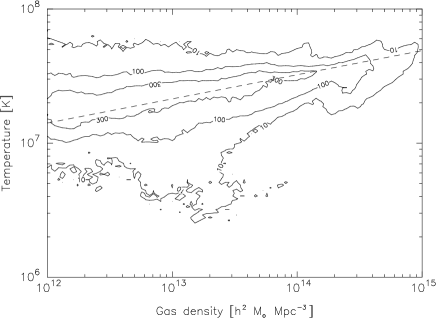
Figure 3: Histogram of individual gas particles of Cluster A in the $\rho_{\rm g}-T$ plane. Contour lines are drawn at 10, 100 and 300 particles per bin. Dashed line shows the expected slope for $\gamma=1.18$.

Gas in small haloes is typically much colder than the intracluster medium. Cold gas clumps corresponding to infalling galaxies can be distinctly appreciated in Figure 3, but their mass is too low to alter the effective polytropic index of Cluster A. However, the profiles become very noisy beyond the virial radius, as well as in major mergers. A constant $\gamma$ is not an accurate approximation in these cases, where the amount of substructure within a spherical shell is large.

3.2 Cluster models based on a ’universal’ CDM density profile

As pointed out in Makino et al. (1998) and Suto et al. (1998), the gas density and temperature profiles can be derived analytically from the CDM mass distribution under the assumptions of hydrostatic equilibrium and a polytropic equation of state. In the present work, we will consider the functional forms proposed by NFW,

$$\rho_{\rm dm}^{\rm NFW}(r)=\frac{\rho_{\rm s}}{(r/r_{\rm s})(1+r/r_{\rm s})^{2}}$$ (8)

and MQGSL,

$$\rho_{\rm dm}^{\rm MQGSL}(r)=\frac{\rho_{\rm m}}{(r/r_{\rm m})^{3/2}\left[1+(r/r_{\rm m})^{3/2}\right]}$$ (9)

Gas density and temperature profiles can be computed by substituting these mass distributions into equation (1) and combining it with equation (2). Following the notation of Suto et al. (1998), the gas temperature is given by

$$\frac{T(r)}{T_{0}}=1-B_{\rm i}f_{\rm i}(r/r_{\rm i})$$ (10)

where the subscript ’i’ can be either ’s’ or ’m’ for NFW and MQGSL models,

$$f_{\rm s}(x)=1-\frac{\ln(1+x)}{x}$$ (11)

and

$$f_{\rm m}(x) = \frac{\pi}{3\sqrt{3}}+\frac{2}{\sqrt{3}}\arctan\left(\frac{2x^{1/2}-1}{\sqrt{3}}\right)$$ (12)

$$+\frac{1}{3}\ln\left(\frac{x+2x^{1/2}+1}{x-x^{1/2}+1}\right)-\frac{2\ln(1+x^{3/2})}{3x}$$

In both cases,

$$B_{i}=\frac{4\pi G\mu m_{\rm p}(\gamma-1)\rho_{\rm i}r_{\rm i}^{2}}{\gamma kT_{0}}$$ (13)

relates the central temperature $T_{0}$ to the underlying dark matter distribution. The gas density can be easily obtained from the polytropic relation

$$\frac{\rho_{\rm g}(r)}{\rho_{0}}=\left[\frac{T(r)}{T_{0}}\right]^{1/(\gamma-1)}$$ (14)

According to this simple picture, clusters of galaxies can be described as a function of 5 parameters. A characteristic density and radius define the properties of the CDM halo, whereas for the ICM we also need to specify the gas density and temperature at $r=0$, as well as the polytropic index $\gamma$.

However, equation (13) relates the values of these variables. The number of free parameters can be further reduced by imposing additional constraints. For instance, Komatsu & Seljak (2001) choose $T_{0}$ and $\gamma$ by enforcing approximately constant baryon fraction at large radii. In our case, we just impose vanishing density at infinity, i.e. $B_{\rm s}=1$ and $B_{\rm m}=3\sqrt{3}/(4\pi)$, and we compute the central gas density from the condition that the baryon fraction never exceeds the cosmic value,

$$\frac{\rho_{\rm g}(r_{\rm max})}{\rho_{\rm dm}(r_{\rm max})}=\frac{\Omega_{\rm b}}{\Omega_{\rm dm}}$$ (15)

where $r_{\rm max}$ is the radius at which the predicted baryon fraction reaches its maximum ($2.71r_{\rm s}$ or $1.34r_{\rm m}$). With this prescription,

$$\rho_{0}^{\rm NFW}\simeq 1.51\frac{\Omega_{\rm b}}{\Omega_{\rm dm}}\rho_{\rm s}~{}~{},~{}~{}\rho_{0}^{\rm MQGSL}\simeq 23.08\frac{\Omega_{\rm b}}{\Omega_{\rm dm}}\rho_{\rm m}$$ (16)

In principle, there is no reason why the baryon fraction cannot exceed the cosmic value somewhere within the cluster. Yet, our numerical results (see Section 4.3 below) indicate that the gas to dark matter ratio increases monotonically (i.e. $r_{\rm max}=\infty$) up to $\Omega_{\rm b}/\Omega_{\rm dm}$. Since the analytical estimate obtained for NFW and MQGSL models does not tend to an asymptotic value, we decided to set the normalisation at the maximum. The value of $\rho_{0}$ varies by $\sim 25$ per cent for any choice between $r_{\rm max}$ and $R_{200}$, but inaccuracies in the assumption of thermally-supported hydrostatic equilibrium might bias a prescription based on large radii.

The last parameter in this family of models is the polytropic index $\gamma$. According to our results (see Figure 2), we set it to $\gamma=1.18$. Although this value is consistent with recent observations (e.g. Markevitch et al., 1998; Sanderson et al., 2003), it would be interesting to investigate its physical origin, as well as whether it can be related to other parameters such as halo mass or concentration. However, such a study requires a much larger number of objects, over a broader mass range, in order to be statistically significant.

3.3 $\beta$-models

Most observational studies do not explicitly rely on the assumption of a given CDM density profile. Instead, they fit the observed X-ray surface brightness with equation (4), and then compute the dark and baryonic profiles by applying hydrostatic equilibrium and a polytropic (often isothermal) equation of state.

To a great extent, the so-called ’$\beta$-discrepancy’ is due to the fact that expression (3) does not provide a good fit to the gas distribution throughout the whole cluster (see e.g. Navarro et al., 1995; Bartelmann & Steinmetz, 1996). Mathiesen & Evrard (2001) argue that line emission from cold gas in the outskirts of the cluster is entirely responsible for the observed value $\beta\sim 2/3$.

Polytropic $\beta$-models have also been proposed to account for the presence of a temperature gradient, but equation (3) is still used to model the gas density (e.g. Ettori, 2000). In the general polytropic case, the surface brightness

$$S_{\rm X}(\theta)=S_{0}\left[1+(\theta/r_{\rm c})^{2}\right]^{1/2-3\beta(1+\frac{\gamma-1}{4})}$$ (17)

is similar to the conventional form (4) for any reasonable value of the polytropic index ($1<\gamma<5/3$). Therfore, the gas density inferred from a fit to the observed X-ray profile has virtually the same shape in both the isothermal (BM) and polytropic (PBM) $\beta$-models. The central surface brightness is given by

$$S_{0}=\sqrt{\pi}\rho_{0}^{2}r_{\rm c}\lambda T_{0}^{1/2}\frac{\Gamma[3\beta(1+\frac{\gamma-1}{4})-1/2]}{\Gamma[3\beta(1+\frac{\gamma-1}{4})]}$$ (18)

Hydrostatic equilibrium leads to an underlying mass distribution

$$M(r)=\frac{3\beta kT_{0}\gamma r_{\rm c}}{G\mu m_{\rm p}}(r/r_{\rm c})^{3}\left[1+(r/r_{\rm c})^{2}\right]^{-3\beta(\gamma-1)/2-1}$$ (19)

which features a finite central density

$$\rho_{\rm dm}(0)\equiv\rho_{\beta}=\frac{9\beta kT_{0}\gamma}{4\pi G\mu m_{\rm p}r_{\rm c}^{2}}$$ (20)

Therefore, the structure of the dark matter halo in the $\beta$-model is related to gas temperature in a way analogous to the models described above. We can follow the same procedure to normalise the central gas density, imposing that the maximum baryon fraction equals the cosmic value. We will consider a standard $\beta$-model ($\gamma=1$) with $\beta=2/3$ and a polytropic form with $\gamma=1.18$ and $\beta=1$. For these values, the maximum baryon fraction occurs at $r_{\rm max}^{\rm BM}\to\infty$ and $r_{\rm max}^{\rm PBM}\simeq 4.18r_{\rm c}$, respectively, and hence

$$\rho_{0}^{\rm BM}=\frac{1}{3}\frac{\Omega_{\rm b}}{\Omega_{\rm dm}}\rho_{\beta}~{}~{},~{}~{}\rho_{0}^{\rm PBM}\simeq 0.39\frac{\Omega_{\rm b}}{\Omega_{\rm dm}}\rho_{\beta}$$ (21)

	NFW	MQGSL	BM / PBM
$\rho_{\rm dm}(x)$	$x^{-1}(1+x)^{-2}$	$x^{-3/2}(1+x^{3/2})^{-1}$	$\left[1+(\frac{1}{3}-B)x^{2}\right](1+x^{2})^{-3B/2-2}$
$M_{\rm dm}(x)$	$\ln(1+x)-x(1+x)^{-1}$	$\frac{2}{3}\ln(1+x^{3/2})$	$\frac{1}{3}x^{3}(1+x^{2})^{-3B/2-1}$
$\rho_{\rm g}(x)$	$\left[x^{-1}\ln(1+x)\right]^{1/(\gamma-1)}$	$\left[1-\frac{3\sqrt{3}}{4\pi}f_{\rm m}(x)\right]^{1/(\gamma-1)}$	$(1+x^{2})^{-3\beta/2}$
$T(x)$	$x^{-1}\ln(1+x)$	$1-\frac{3\sqrt{3}}{4\pi}f_{\rm m}(x)$	$(1+x^{2})^{-3B/2}$

Table 2: Polytropic models of galaxy clusters in hydrostatic equilibrium. $x$ denotes the radial coordinate in units of the characteristic radius of each model ($r_{\rm s}$ in NFW, $r_{\rm m}$ in MQGSL, and $r_{\rm c}$ in $\beta$-models). Dark matter density is scaled in terms of the characteristic density ($\rho_{\rm s}$, $\rho_{\rm m}$, and $\rho_{\beta}$, respectively). Masses are in units of $4\pi\rho_{\rm i}r_{\rm i}^{3}$. Gas density and temperature are scaled by their central values $\rho_{0}$ and $T_{0}$. The abbreviations $f_{\rm m}(x)$, given by (12), and $B\equiv\beta(\gamma-1)$ have been used.

We quote in Table 2 the distributions of dark and baryonic matter expected in our four analytical cluster models. Cumulative gas mass and projected quantities in NFW and MQGSL must be integrated numerically. Relations between the characteristic parameters are summarised in Table 3.

Model	$S_{0}/(\lambda\rho_{0}^{2}T_{0}^{1/2}r_{\rm i})$	$(\Omega_{\rm b}\rho_{\rm i})/(\Omega_{\rm dm}\rho_{0})$	$T_{0}/(4\pi G\mu m_{\rm p}\rho_{\rm i}r_{\rm i}^{2})$
NFW	0.191	1.51	0.153
MQGSL	0.0151	23.08	0.369
BM	1.571	1/3	6
PBM	1.145	0.39	10.62

Table 3: Relations between the characteristic radius $r_{\rm i}$, CDM density $\rho_{\rm i}$, gas density $\rho_{0}$, and gas temperature $T_{0}$. All quantities have been computed assuming $\gamma=1.18$, except in the BM ($\gamma=1$). For this model, $\beta=2/3$; for PBM, $\beta=1$.

4 Results

We have shown that our clusters are, to a fair extent, in hydrostatic equilibrium, and that a polytropic equation of state with $\gamma=1.18$ provides a good description of the hot diffuse component of the ICM. Under these conditions, models of the radial structure of galaxy groups and clusters can be derived from phenomenological approaches to either the gas or dark matter density. In this Section, we compare these simple, self-consistent models with the spherically-averaged distributions of mass, gas density and temperature found in our sample of simulated galaxy clusters.

For NFW and MQGSL, we fit the cumulative dark mass of each halo, while for the $\beta$-models the gas mass is used instead. We compute the numerical profiles in 26 logarithmic bins between $0.05R_{200}$ and $R_{200}$. We set the lower cut-off well above our resolution limit ($\sim 0.01R_{200}$) not only to avoid numerical effects but also to investigate how accurate are the extrapolations of the analytical cluster models towards $r=0$.

The parameter space is explored by letting $r_{200}$ and $c_{\rm i}\equiv r_{200}/r_{\rm i}$ vary uniformly in the range $0.25<r_{200}<1.25\ h^{-1}$ Mpc and $0.1<c_{\rm i}<16$ (50 for BM). For the gas mass, the radius $r_{10}$ (enclosing a mean density of $10\rho_{\rm c}$) is used instead of $r_{200}$. Both quantities are roughly equivalent for the baryon fraction assumed in this work.

Figure 4: Best-fitting model parameters for our sample of numerical galaxy clusters (see text for details on the fitting procedure). Solid squares represent relaxed objects, empty squares are used for minor mergers and stars for major merging systems. Contours indicate $\sqrt{\chi^{2}/(dof)}=0.1$. Dashed line in NFW panel plots $c=6.8r_{\rm 200}^{-0.3}$.

Results of the $\chi^{2}$ minimisation are plotted in Figure 4. In most cases, the quality of the fit is only slightly better for NFW and MQGSL models ($\sqrt{\chi^{2}/(dof)}\sim 0.05-0.1$) than for $\beta$-models ($0.05-0.15$). Best-fitting values of $r_{200}$ are close to the actual $R_{200}$ (quoted in Table 1) obtained directly from the simulated mass profile. The values of $r_{10}$ in BM ($\beta=2/3$) are less well correlated with $R_{200}$ than those obtained for PBM ($\beta=1$).

Although the full sample is consistent with constant dark matter concentration over the restricted mass range probed, we notice a well-defined bimodal behaviour: while relaxed clusters follow the usual relation, approximated by $c=186M_{200}^{-0.1}$ for the NFW profile (Burkert & Silk, 1999), mergers are dramatically offset down, particularly low-mass systems. In the $\beta$-models, we find that the best-fitting gas concentration even increases with cluster mass. In several systems, the core radius inferred by the BM is only slightly larger than the innermost radial bin included in the fit.

An important fact is that dark and baryonic matter distributions are expected to be strongly correlated, by virtue of the hydrostatic equilibrium equation and the constraint of a cosmic baryon fraction. All analytical models of galaxy groups and clusters studied in the present work have only two free parameters. According to our fitting procedure, gas density and temperature are genuine predictions (i.e. not fits) of the models based on a dark matter profile. Conversely, the same is true for the CDM density and gas temperature in the $\beta$-models.

4.1 Mass distribution

The radial density profiles of our dark matter haloes are shown on the left panel of Figure 5, rescaled by their best-fitting characteristic densities and radii. We plot the expected mass distribution in each model (see Table 2) as a solid line. On the right panel, we plot the accuracy of the analytical estimates, defined as

$$\frac{\Delta\rho_{\rm dm}}{\rho_{\rm dm}}\equiv\frac{\rho_{\rm est}(r)-\rho_{\rm num}(r)}{\rho_{\rm num}(r)}$$ (22)

where $\rho_{\rm est}$ and $\rho_{\rm num}$ are the estimated and numerical profiles, respectively.

Figure 5: Dark matter density profile of our numerical haloes. Black squares represent the average over all clusters, excluding major mergers. Error bars indicate one-sigma scatter of individual profiles. Left panel: CDM density, scaled by the best-fitting $\rho_{\rm i}$ and $r_{\rm i}$ of each object in the corresponding model. Analytical profiles are shown as solid lines. Right panel: Accuracy of each analytical profile. Vertical dotted lines mark the fitted region.

Not surprisingly, both NFW and MQGSL offer an excellent fit to the dark matter distribution, but the core-like predictions of the $\beta$-models represent a very poor approximation to the numerical profiles. The conventional $\beta$-model has a much better accuracy throughout the fitted range, but the extrapolation to larger radii is more reliable in the polytropic version, thanks to its higher value of $\beta$.

Concerning the controversy about the inner slope of the density profile, it is apparent from Figure 5 that MQGSL formula is slightly more accurate than NFW near the centre, albeit the scatter of individual profiles around the average is somewhat higher. This issue is addressed in more detail in Figure 6, where we plot the logarithmic slopes of the CDM density and cumulative mass profiles, computed directly from the simulation data

$$\alpha_{\rho}=\frac{{\rm d}\log[\rho_{\rm dm}(r)]}{{\rm d}\log(r)}~{}~{},~{}~{}\alpha_{\rm M}=\frac{{\rm d}\log[M_{\rm dm}(r)]}{{\rm d}\log(r)}$$ (23)

Figure 6: Logarithmic slope of the CDM mass (top) and density (bottom) profiles. Squares with error bars represent the average over relaxed clusters and minor mergers. Analytical cluster models are shown as lines.

In general terms, both NFW and MQGSL formulae are consistent with our results up to the resolution limit. When we divide our sample according to the dynamical state of each cluster, we find a well defined trend in the sense that relaxed haloes display shallower central slopes (close to NFW) than merging systems (better described by MQGSL). As an extreme case, major mergers feature pure power-law mass distributions for more than one decade in radius, whose slopes are even steeper than the value proposed by MQGSL. In agreement with Power et al. (2003), we do not find any sign of an asymptotic slope for either relaxed clusters or minor mergers. More resolution is clearly required before achieving a firm conclusion on this matter.

4.2 Gas temperature

Mass determinations from X-ray emission in clusters usually assume that relaxed clusters (i.e. morphologically symmetric) are isothermal. However, this assumption has been questioned recently by Markevitch et al. (1998), who found evidence of a decreasing temperature profile for nearby clusters observed with ASCA. This result has been confirmed for cool clusters by Finoguenov et al. (2001). On the contrary, White (2000) and Irwin & Bregman (2000), using data from BeppoSAX and ASCA satellites, do not find any decrease of the temperature in a large collection of clusters. More recently, the analysis of BeppoSAX observations accomplished by De Grandi & Molendi (2002) concluded that temperature profiles of galaxy clusters can be described by an isothermal core followed by a rapid decrease.

Numerical simulations of galaxy clusters support a significant decrease in the ICM temperature from the central regions to the virial radius (e.g. Frenk et al., 1999). Recent results from high resolution AMR gasdynamical simulations seem to indicate that the temperature profile has an universal form (Loken et al., 2002). These authors proposed a simple formula to fit the projected emission-weighted temperature of their clusters:

$$T_{\rm p}^{\rm X}(\theta)=T_{0}{(1+\theta/a_{\rm x})}^{-\delta}$$ (24)

where $T_{0}$ is the central temperature and $a_{\rm x}$ a core radius. Loken et al. (2002) quote best-fitting values of these parameters $a_{\rm x}=r_{\rm vir}/1.5$ and $\delta=1.6$.

Figure 7: Same as Figure 5, for the temperature profile.

The average mass-weighted temperature profile of our sample of galaxy clusters (excluding major mergers) is shown on the left panel of Figure 7. The normalisation $T_{0}$ has been computed analytically from the fit to the dark matter (NFW, MQGSL) or gas (BM, PBM) distribution of each cluster. As can be seen on the right panel, the theoretical prediction is accurate within $\sim 15$ per cent for all prescriptions, with the obvious exception of the isothermal $\beta$-model. NFW and MQGSL models are virtually indistinguishable.

In order to compare with observations, as well as with the numerical work of Loken et al. (2002), we plot in Figure 8 the average projected X-ray temperature profile. We computed the emission-weighted temperature according to equation (6) in cylindrical shells of 3 $h^{-1}$ Mpc length, oriented along the main axes of the simulation box. The final profile of each cluster is given by the average over the three orthogonal projections, and the normalisation comes from the emission-weighted temperature, $T_{200}^{X}$, within $R_{200}$ (both quantities are quoted in Table 1).

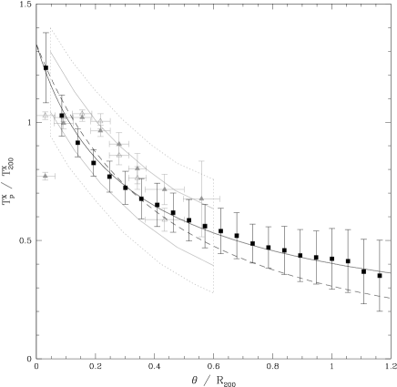
Figure 8: Projected emission-weighted temperature profile, scaled by $T_{200}^{\rm X}$ in Table 1 (black squares with error bars). Solid line is the best fit obtained with equation (24), dashed line represents the simulation results of Loken et al. (2002). Observational data from De Grandi & Molendi (2002) are shown as triangles (filled for cooling flow and empty for non-cooling flow clusters). Dotted box encloses the temperature profiles observed by Markevitch et al. (1998) plus most of the error bars, solid box includes only the scatter of their best-fitting polytropic models.

Our results are in excellent agreement with the observational estimate of Markevitch et al. (1998), who claim that the emission-weighted temperature is well represented by a polytropic $\beta$-model (indeed, our data are almost identical to their best-fitting profile). However, our profiles are only marginally consistent with the results reported by De Grandi & Molendi (2002). In particular, we do not find any evidence of the temperature flattening observed by these authors at $r\sim 0.2R_{200}$.

The projected X-ray temperature of our clusters rises uninterruptedly until the innermost radial bin, in agreement with the results of Eulerian codes, such as ART (see Section 2.2) or that employed by Loken et al. (2002). Equation (24) fits well our numerical data, but we obtain rather different values of the core radius and the asymptotic exponent, $a_{\rm x}=r_{200}/4.5$ and $\delta=0.7$. Since both simulated temperature profiles are consistent within the error bars, it seems that the best-fitting values of $a_{\rm x}$ and $\delta$ are rather sensitive to the details of the data.

Never the less, we would like to stress that a decreasing temperature profile is a robust result of numerical simulations regardless of the integration scheme (either AMR or SPH), as long as entropy conservation is enforced in the latter. Furthermore, such behaviour is strongly supported by most recent observational measurements. The presence of an isothermal core in the observed galaxy clusters could reflect the need for additional non-adiabatic physics in the simulations.

4.3 Gas density

Finally, we compare the simulated gas density profile with the distributions expected in our four analytical cluster models. It is evident from Figure 9 that the discrepancies are remarkably larger than for the dark matter density or ICM temperature profiles.

Figure 9: Same as Figure 5, for the gas density profile.

It is somewhat surprising that the $\beta$-models show the worst inconsistencies with the data, since they are specifically intended to fit the gas distribution. When $\beta=2/3$, the asymptotic gas density falls too slowly, as $r^{-2}$. However, the central regions cannot be properly fitted if $\beta=1$ is assumed. The final outcome is that the best-fitting value of $\beta$ increases from one value to the other as larger radii are considered in the fit.

Models based on a ’universal’ dark matter profile provide a fair description of the ICM density. None the less, we caution that in many cases the simulated gas density can differ substantially from the analytical prediction, giving rise to the huge scatter ($\sim 40$ per cent) observed in Figure 9. On one hand, the CDM distribution at small radii depends on the dynamical state of the halo. Near the virial radius, even relaxed clusters deviate noticeably from thermally-supported hydrostatic equilibrium (see Figure 2), and we also observe that the dark matter density is slightly higher than indicated by both NFW and MQGSL formulae (see Figure 5). More importantly, the polytropic index is not exactly the same for all clusters, which strongly alters the shape of the inferred gas density profile.

Inaccuracies in the estimated dark matter and/or gas profiles lead to a significant mismatch between the analytical and numerical baryon fractions. The local ratio of gas to CDM density is plotted in Figure 10 as a function of radius, rescaled by the cosmic value. None of the analytical cluster models is able to fit satisfactorily the simulated profile. The canonical $\beta$-model is the only scenario in which the baryon fraction reaches an asymptotic value, but this is due to the equally wrong gas and dark matter densities. In the other models, the baryon fraction reaches a maximum around three times the characteristic radius, but then it drops rather steeply.

Figure 10: Same as Figure 5, for the local baryon fraction.

We used this maximum to find out the normalisation of the ICM density, $\rho_{0}$. However, the steep asymptotic slope of the gas density profile hints that more realistic models have to be considered in order to reproduce the radial structure near the virial radius. On the other hand, such a modelisation (e.g. including departures from spherical symmetry, infall and turbulent motions) would introduce additional free parameters that would complicate the physical interpretation of the results.

5 Observable consequences

Analytical models of galaxy groups and clusters are a key ingredient in the interpretation of observational data, since they relate the X-ray emission of the ICM to the underlying gas and dark matter distributions. In particular, X-ray observations are usually restricted to the central regions, and these models allow the extrapolation of the spherically-averaged profiles up to the virial radius. In some occasions, they are also extrapolated inwards, in order to correct for the presence of a central cooling flow. Quite often, the virial radius itself is derived by assuming a particular model.

Therefore, we would like to investigate in some detail to what extent the assumed radial structure can bias the conclusions drawn from observational studies. We construct X-ray surface brightness profiles in the same manner as we did for the projected emission-weighted temperature (i.e. assuming pure bremsstrahlung radiation and averaging over the three axes). Then, we fit the simulated profiles with our four analytical models, varying the projected characteristic radius, $\theta_{\rm i}$, and the central surface brightness, $S_{0}$. Results are shown in Figure 11.

Figure 11: Best-fitting values of the central X-ray surface brightness, $S_{0}$, and the projected characteristic radius, $\theta_{\rm i}$. Solid squares are used for relaxed systems, empty squares for minor mergers and stars for major mergers. Contours are drawn at $\sqrt{\chi^{2}/(dof)}=0.2$.

Only data between 0.05 and 0.5 $R_{200}$ were used. The lower cut-off is similar to region excised in observational studies to avoid the cooling flow region. The upper scale is similar to that attained by X-ray data. Furthermore, we find that the emission at larger radii is significantly enhanced by small mass subhaloes, which manifest as peaks in the surface brightness. We discard these features by fitting only those bins that lead to a monotonically decreasing profile. As pointed out by Mathiesen & Evrard (2001), the inclusion of emission lines would still increase the contribution of substructure to the total X-ray luminosity.

The dependence of the fit on the choice of the outer radius $R_{\rm out}$ is plotted in Figure 12. NFW and MQGSL models are more stable than $\beta$-models, and their best-fitting $\theta_{\rm i}$ are much closer to the actual characteristic radius $r_{\rm i}$, computed from the mass distribution between 0.05 $R_{200}$ and $R_{200}$ (see Section 4). The conventional $\beta$-model offers a poor fit to our simulated surface brightness at large radii, due to the shallow slope associated to $\beta=2/3$. For several objects, the best fit is obtained with the lowest possible $\theta_{\rm c}$ (i.e. a pure power law, $S_{\rm X}\propto r^{-1.5}$). Since we assumed $\beta=1$ for the PBM, a better agreement is found with the numerical results, although the best-fitting $\theta_{\rm c}$ is systematically higher than the core radius inferred from the gas mass.

Figure 12: Dependence on the outer radius, $R_{\rm out}$, used for the fit to the X-ray surface brightness profile. Solid lines represent NFW model; dotted, MQGSL; short-dashed, BM; long-dashed, PBM. Left panel: Projected characteristic radius, divided by the three-dimensional estimation based on the CDM/gas distribution. Right panel: Goodness of the surface brightness fits.

We assume that the characteristic radii of our clusters in each model are equal to their best-fitting projected equivalents, $\theta_{\rm i}$. To obtain the characteristic CDM densities, as well as the central gas densities and temperatures, we must solve a system of equations, which in the $\beta$-model is given by (18), (20) and (21). For the models based on a ’universal’ dark matter density profile, the surface brightness is integrated numerically, yielding the central values quoted in Table 3. They must be combined with equations (13) and (16), substituting the appropriate value of $B_{\rm i}$.

A last interesting point to note is that we are not using any information about the X-ray temperature. In doing so, we could skip one of our constraints, such as the value of the polytropic index or the normalisation of the central gas density with respect to the CDM component.

5.1 X-ray surface brightness

The first question we would like to address is how well can our analytical cluster models fit the X-ray surface brightness. We show in Figure 13 that the numerical profiles are fairly described by NFW or MQGSL, although the accuracy of the fits degrades dramatically at large radii. Never the less, we find that the difference between the analytical and simulated profiles is of the order of $30-40$ per cent up to the virial radius. Some part of it is caused by the low gas density predicted by these models at large radii. The rest is due to the emission of substructure beyond 0.5 $R_{200}$.

Figure 13: X-ray surface brightness, averaged over all clusters except major mergers. Error bars indicate one-sigma scatter of individual profiles. Left panel: Surface brightness profile, scaled by the best-fitting $S_{0}$ and $\theta_{\rm i}$. Analytical cluster models are shown as solid lines. Right panel: Accuracy of each analytical profile. Vertical dotted lines mark the fitted region.

Consistently with observational results, the isothermal $\beta$-model with $\beta=2/3$ provides a fairly good fit to the X-ray surface brightness only for $r\leq 0.3R_{200}$. As was shown for the gas density, the outer parts are better approximated by $\beta\sim 1$. When we let $\beta$ vary as a free parameter, the best fit to our data is obtained by $\beta\sim 0.8$. However, this is a ’compromise solution’ that fails to properly describe the ICM at very small or large radii.

5.2 Mass estimates

One of the most important applications of hydrostatic equilibrium and a polytropic equation of state is the estimate of the cumulative mass profile of both dark and baryonic components, given the observed X-ray emission. We plot in Figure 14 the CDM mass distribution inferred for our cluster sample (excluding major mergers), scaled by the characteristic densities and radii derived from the fit to the surface brightness profile.

Figure 14: Dark matter mass profile, inferred from the X-ray surface brightness. Symbols as in Figure 13.

The accuracy of the mass estimate is similar in all models ($\sim 20$ per cent errors), but the shape of the mass distribution is substantially more accurate when a NFW or MQGSL ’universal’ CDM density profile is assumed. The isothermal $\beta$-model gives an acceptable estimate of the dark matter mass for $0.1<r/R_{200}<1$ because of the small values inferred for the core radius. In the PBM, this quantity is substantially higher and thus a ’core’ in the dark matter distribution can be noticed for $r\leq 0.3R_{200}$.

Cumulative gas mass estimates are plotted in Figure 15. In this case, the small values of $r_{\rm c}$ in the BM lead to extremely high central densities, whereas the PBM (with $\beta=1$) predicts an excessively large core. Again, a profile closer to the numerical results can be obtained by treating $\beta$ as a free parameter. The estimates based on a ’universal’ CDM profile are only slightly more accurate. The scatter, as well as the overall shape, are greatly improved by considering individual values of the polytropic index.

Figure 15: Same as Figure 14, for the cumulative gas mass.

Regarding the total baryon fraction, we can see in Figure 16 that the $\beta$-models can lead to severe overestimates of this quantity at small radii ($r\leq 0.1-0.3\ R_{200}$). Near the virial radius, though, uncertainties are of the order of 10 per cent. NFW and MQGSL models are accurate within $\sim 20$ per cent for $r\geq 0.2R_{200}$ and $\sim 50$ percent as we move closer to the centre.

Figure 16: Same as Figure 14, for the cumulative baryon fraction in units of the cosmic value.

Another (sometimes more important) source of uncertainty comes from the estimation of the virial radius itself. Furthermore, $R_{200}$ is not a fixed multiple of the characteristic radius in any analytical model of galaxy clusters, and hence the cumulative baryon fraction at a fixed overdensity is extremely sensitive to halo concentration, particularly at low radii. Assuming a NFW model, the baryon fraction within $R_{200}$ can change by less than 10 per cent from $c=4$ to $c=9$, but at 0.1 $R_{200}$, the ratio of gas to dark matter mass varies from .5 to .75 times the cosmic value.

5.3 Entropy

Entropy plays a fundamental role in clusters of galaxies because convection acts as an entropy-sorting device, moving low entropy material to the cluster core and high entropy material to the outskirts. Gas density and temperature in hydrostatic and convective equilibrium are just manifestations of the underlying entropy distribution. The claim of an entropy floor in small groups (Ponman et al., 1999) has often been regarded as evidence of preheating of the ICM at high redshift. Using a much larger sample, Ponman et al. (2003) find that the observed profiles appear to be approximately self-similar apart from a normalisation constant. They obtain a best-fit behaviour $S(0.1R_{200})\propto T^{0.65}$ for systems spanning a temperature range from 1 to 10 keV.

The entropy profile has recently been studied by Borgani et al. (2001) and Finoguenov et al. (2003) by means of numerical simulations that include cooling and preheating. With gravitational heating alone, these authors find a power-law entropy profile, consistent with other results based on the standard implementation of SPH (see e.g. Frenk et al., 1999). As was discussed in Section 2.2, the situation changes dramatically when entropy conservation is explicitly enforced, either in the SPH algorithm or in Eulerian schemes. Shock heating becomes substantially more efficient, leading to a much higher entropy near the cluster centre, as well as stripping low-entropy gas from the infalling galaxies that otherwise would survive for several crossing times (Borgani et al., 2001).

We plot our entropy profiles in Figure 17. As expected for a polytropic gas in hydrostatic equilibrium, they are not pure power laws for any reasonable choice of the ’universal’ gas or dark matter distribution. Furthermore, the shape of the entropy profile does not depend systematically on the mass or temperature of the object, in agreement with recent observations (Ponman et al., 2003). NFW or MQGSL models provide a much better estimate of the entropy distribution than any version of the $\beta$-model. However, the low gas densities predicted at large radii yield a slope at $r\sim R_{200}$ significantly steeper than the numerical data.

Figure 17: Same as Figure 14, for the entropy profile. Entropy is defined as $S=kTn_{e}^{-2/3}$ and rescaled by the central values of the ICM density and temperature inferred from the fit to the X-ray surface brightness.

Given our limited temperature coverage, the normalisation of the entropy profiles is consistent within the error bars with both the self-similar scaling ($S\propto T$) as well as with the observed trend, $S\propto T^{0.65}$. In any case, we would like to stress that we do not expect to find the self-similar scaling albeit we are neglecting non-gravitational processes. The central entropy in any model scales as $T_{0}\rho_{0}^{-2/3}$, where $\rho_{0}\propto\rho_{\rm i}$ and $T_{0}\propto\rho_{\rm i}r_{\rm i}^{2}$. Recovering a normalisation exactly proportional to the central temperature would require that the characteristic CDM density was independent on halo mass (i.e. constant concentration).

As in the baryon fraction, we argue that the characteristic density and radius can be more physically meaningful than the mass and radius at a given overdensity. Depending on concentration, the entropy at some fraction of $R_{200}$ can vary as much as a factor of 3. This can have important consequences on the $S-T$ relation, since we have shown that merging systems are systematically much less concentrated than relaxed haloes of the same mass. A lower concentration implies a lower central gas density, but also a lower temperature and a smaller value of $R_{200}/r_{\rm i}$. Therefore, the net effect depends on the details of the mass-concentration relation.

Figure 18: Gas entropy at 0.1 $R_{200}$ versus emission-weighted temperature. Solid squares represent relaxed clusters, empty squares are used for minor mergers and stars for major merging systems. Solid line depicts the self-similar scaling, $S\propto T$, while dashed line shows the observed behaviour, $S\propto T^{0.65}$.

The $S-T$ relation for our sample of numerical clusters is shown in Figure 18. The entropy, $S=kT[\rho_{\rm g}/(\mu m_{\rm p})]^{-2/3}$, is evaluated at 0.1 $R_{200}$ and plotted as a function of the X-ray temperature of the object (see Table 1). Systems that have been catalogued as mergers according to our substructure criterium display higher entropies than relaxed clusters. Since mergers are more common on group scales, the $S-T$ relation becomes considerably flattened when these systems are taken into account.

6 Conclusions

In this paper, we have considered four self-consistent analytical models of galaxy clusters, based on the hypotheses that the hot ICM gas is in hydrostatic equilibrium with the dark matter halo and that it follows a polytropic equation of state. Two of our models assume NFW and MQGSL formulae to describe the CDM density profile, whereas the other two assume a $\beta$-model for the gas distribution. One is an isothermal version with $\beta=2/3$ (BM) and the other is a polytropic model with $\gamma=1.18$ and $\beta=1$ (PBM).

We performed a set of high-resolution adiabatic gasdynamical simulations to assess the accuracy of the basic approximations (i.e. hydrostatic equilibrium and a polytropic relation). Then, we compared the radial distributions of gas and dark matter expected in each analytical model with the results for a sample of 15 numerical groups and clusters between 1 and 3 keV.

Our main conclusions can be summarised as follows:

1. We find additional evidence of non-physical entropy losses in the standard implementation of the SPH algorithm. This effect can be of critical importance in the computation of the temperature and entropy profiles. The new formulation proposed by Springel & Hernquist (2002) appears to be a promising alternative to overcome this problem.

2. Thermally-supported hydrostatic equilibrium is a valid approximation for objects classified as ’relaxed’ on dynamical grounds, up to $\sim 0.8R_{200}$. We find evidence of non-thermal support in merging systems.

3. A polytropic equation of state with $\gamma\sim 1.18$ provides a fairly good description of the ICM gas. Substructure induces deviations from this relation.

4. The density profile of our clusters can be well fitted by either NFW or MQGSL formulae. $\beta$-models predict constant dark matter density near the centre, in conflict with the numerical results. Major mergers feature a power-law density profile with slope $-2\leq\alpha\leq-1$.

5. Gas temperature declines by a factor of $2-3$ from the centre to the virial radius. Our projected X-ray temperature profiles can be fitted by the ’universal’ form proposed by Loken et al. (2002), derived from Eulerian gasdynamical simulations, although we obtain different values for the free parameters. Purely adiabatic physics cannot account for a large isothermal core.

6. $\beta$-models fail to reproduce the gas density profile. While a fit to the inner part yields $\beta\sim 2/3$, larger values are required at large radii. NFW and MQGSL models are able to predict the average distribution, but variations in the polytropic index lead to a very large scatter. The asymptotic slope of the gas density profile is too steep compared to the simulation data.

7. Models based on a ’universal’ CDM profile are able to estimate the ICM properties within $30-40$ per cent errors, when applied to the simulated X-ray surface brightness. Assuming a $\beta$-model yields similar estimates for $r\geq 0.1R_{200}$, but the shape of the inferred profiles at smaller radii can be severely misleading.

8. Contrary to conventional SPH estimates, the entropy distribution is not a pure power law. All our analytical cluster models predict an increasing slope with radius, consistent with our numerical data. The entropy profile is entirely determined by the characteristic density and radius of the CDM halo, and the normalisation depends on the mass-concentration relation. In particular, it does not necessarily scale linearly with gas temperature.

   In general terms, we claim that the radial structure of galaxy groups and clusters can be understood in terms of hydrostatic equilibrium and a polytropic equation of state for the gas, at least when only gravitational processes and adiabatic gasdynamics are considered.

   Although $\beta$-models can sometimes provide a fair estimate of several cluster properties, they fail to provide an overall description that matches all the numerical data. Models based on a ’universal’ CDM density profile have a similar or better accuracy, and they are far more reliable in a qualitative sense (i.e. concerning the shape of the profiles). We argue that these models are preferable in order to analyse and interpret observational data.

Appendix A Cluster Atlas

In the following image, we display our 15 simulated clusters, projected along the three major axes. Colours indicate the dark matter surface density along the line of sight. Contour plots represent the X-ray emission in conventional units.

Quite interestingly, it can be appreciated that many images of merging systems (both minor and major) appear to be spherically symmetric due to projection effects. Usually, a lot more substructure is present in the CDM density (which roughly corresponds to the optical emission) than in the hot ICM gas (X-ray).

Indeed, we find that the gaseous component of infalling galaxies is very efficiently stripped, while dark matter haloes are able to survive during many orbits around the cluster centre . We expect these haloes to retain some of their original gas when cooling is taken into account, probably undergoing an intense star formation burst. However, all gas in a warm-hot reservoir is lost during the first orbit, quenching any subsequent star formation activity. Numerical experiments that include self-consistent cooling, star formation and feedback are needed in order to make a quantitative assessment of this scenario.

References

- Ascasibar (2003) Ascasibar Y., 2003, PhD thesis, Universidad Autónoma de Madrid (Spain), (astro-ph/0305250)
- Bartelmann & Steinmetz (1996) Bartelmann M., Steinmetz M., 1996, MNRAS, 283, 431
- Bialek et al. (2001) Bialek J. J., Evrard A. E., Mohr J. J., 2001, ApJ, 555, 597
- Borgani et al. (2001) Borgani et al. 2001, ApJ, 559, L71
- Borgani et al. (2002) Borgani et al. 2002, MNRAS, 336, 409
- Bryan & Norman (1995) Bryan G. L., Norman M. L., 1995, Bulletin of the American Astronomical Society, 27, 1421
- Bryan & Norman (1998) Bryan G. L., Norman M. L., 1998, ApJ, 495, 80
- Bryan et al. (1995) Bryan G. L., Norman M. L., Stone J. M., Cen R., Ostriker J. P., 1995, Comput. Phys. Comm., 89, 149
- Burkert & Silk (1999) Burkert A., Silk J., 1999, in Dark matter in Astrophysics and Particle Physics (astro-ph/9904159)
- Cavaliere & Fusco-Femiano (1976) Cavaliere A., Fusco-Femiano R., 1976, A&A, 49, 137
- Cen (1992) Cen R., 1992, ApJS, 78, 341
- Cen et al. (1990) Cen R. Y., Ostriker J. P., Jameson A., Liu F., 1990, ApJ, 362, L41
- Colín et al. (1999) Colín et al. 1999, ApJ, 523, 32
- Davé et al. (2002) Davé R., Katz N., Weinberg D. H., 2002, ApJ, 579, 23
- De Grandi & Molendi (2002) De Grandi S., Molendi S., 2002, ApJ, 567, 163
- Edge & Stewart (1991) Edge A. C., Stewart G. C., 1991, MNRAS, 252, 428
- Eke et al. (1998) Eke V. R., Navarro J. F., Frenk C. S., 1998, ApJ, 503, 569
- Ettori (2000) Ettori S., 2000, MNRAS, 311, 313
- Evrard et al. (1996) Evrard A. E., Metzler C. A., Navarro J. F., 1996, ApJ, 469, 494
- Finoguenov et al. (2001) Finoguenov A., Arnaud M., David L. P., 2001, ApJ, 555, 191
- Finoguenov et al. (2003) Finoguenov et al. 2003, A&A, 398, L35
- Frenk et al. (1999) Frenk et al. 1999, ApJ, 525, 554
- Fukushige & Makino (1997) Fukushige T., Makino J., 1997, ApJ, 477, L9
- Fukushige & Makino (2001) Fukushige T., Makino J., 2001, ApJ, 557, 533
- Ghigna et al. (1998) Ghigna et al. 1998, MNRAS, 300, 146
- Ghigna et al. (2000) Ghigna et al. 2000, ApJ, 544, 616
- Gingold & Monaghan (1977) Gingold R. A., Monaghan J. J., 1977, MNRAS, 181, 375
- Gnedin (1995) Gnedin N. Y., 1995, ApJS, 97, 231
- Gottlöber et al. (2001) Gottlöber S., Klypin A., Kravtsov A. V., 2001, ApJ, 546, 223
- Hernquist (1993) Hernquist L., 1993, ApJ, 404, 717
- Irwin & Bregman (2000) Irwin J. A., Bregman J. N., 2000, ApJ, 538, 543
- Jing & Suto (2000) Jing Y. P., Suto Y., 2000, ApJ, 529, L69
- Kaiser (1986) Kaiser N., 1986, MNRAS, 222, 323
- Klypin et al. (1999) Klypin A., Gottlöber S., Kravtsov A. V., Khokhlov A. M., 1999, ApJ, 516, 530
- Klypin et al. (2001) Klypin A., Kravtsov A. V., Bullock J. S., Primack J. R., 2001, ApJ, 554, 903
- Komatsu & Seljak (2001) Komatsu E., Seljak U., 2001, MNRAS, 327, 1353
- Kravtsov et al. (2002) Kravtsov A. V., Klypin A., Hoffman Y., 2002, ApJ, 571, 563
- Kravtsov et al. (1997) Kravtsov A. V., Klypin A. A., Khokhlov A. M., 1997, ApJS, 111, 73
- Lewis et al. (2000) Lewis et al. 2000, ApJ, 536, 623
- Loken et al. (2002) Loken et al. 2002, ApJ, 579, 571
- Lucy (1977) Lucy L. B., 1977, AJ, 82, 1013
- Makino et al. (1998) Makino N., Sasaki S., Suto Y., 1998, ApJ, 497, 555
- Markevitch et al. (1998) Markevitch M., Forman W. R., Sarazin C. L., Vikhlinin A., 1998, ApJ, 503, 77
- Mathiesen & Evrard (2001) Mathiesen B. F., Evrard A. E., 2001, ApJ, 546, 100
- Moore et al. (1998) Moore B., Governato F., Quinn T., Stadel J., Lake G., 1998, ApJ, 499, L5
- Moore et al. (1999) Moore B., Quinn T., Governato F., Stadel J., Lake G., 1999, MNRAS, 310, 1147
- Motl et al. (2003) Motl P. M., Burns J. O., Loken C., Norman M. L., Bryan G., 2003, ApJ, (astro-ph/0302427)
- Muanwong et al. (2002) Muanwong O., Thomas P. A., Kay S. T., Pearce F. R., 2002, MNRAS, 336, 527
- Nagai & Kravtsov (2002) Nagai D., Kravtsov A. V., 2002, ApJ, submitted (astro-ph/0206469)
- Navarro et al. (1995) Navarro J. F., Frenk C. S., White S. D. M., 1995, MNRAS, 275, 720
- Navarro et al. (1997) Navarro J. F., Frenk C. S., White S. D. M., 1997, ApJ, 490, 493
- Nelson & Papaloizou (1993) Nelson R. P., Papaloizou J. C. B., 1993, MNRAS, 265, 905
- Nelson & Papaloizou (1994) Nelson R. P., Papaloizou J. C. B., 1994, MNRAS, 270, 1
- Neumann & Arnaud (1999) Neumann D. M., Arnaud M., 1999, A&A, 348, 711
- Pearce et al. (2000) Pearce F. R., Thomas P. A., Couchman H. M. P., Edge A. C., 2000, MNRAS, 317, 1029
- Pen (1995) Pen U., 1995, ApJS, 100, 269
- Pen (1998) Pen U., 1998, ApJS, 115, 19
- Ponman et al. (1999) Ponman T. J., Cannon D. B., Navarro J. F., 1999, Nature, 397, 135
- Ponman et al. (2003) Ponman T. J., Sanderson A. J. R., Finoguenov A., 2003, MNRAS, accepted (astro-ph/0304048)
- Power et al. (2003) Power et al. 2003, MNRAS, 338, 14
- Rosati et al. (2002) Rosati P., Borgani S., Norman C., 2002, ARA&A, 40, 539
- Sanderson et al. (2003) Sanderson et al. 2003, MNRAS, 340, 989
- Sarazin (1986) Sarazin C. L., 1986, Reviews of Modern Physics, 58, 1
- Serna et al. (1996) Serna A., Alimi J.-M., Chieze J.-P., 1996, ApJ, 461, 884
- Serna et al. (2003) Serna A., Domínguez-Tenreiro R., Sáiz A., 2003, MNRAS, submitted
- Shapiro et al. (1996) Shapiro P. R., Martel H., Villumsen J. V., Owen J. M., 1996, ApJS, 103, 269
- Springel & Hernquist (2002) Springel V., Hernquist L., 2002, MNRAS, 333, 649
- Springel et al. (2001) Springel V., Yoshida N., White S. D. M., 2001, New Astronomy, 6, 79
- Suto et al. (1998) Suto Y., Sasaki S., Makino N., 1998, ApJ, 509, 544
- Tornatore et al. (2003) Tornatore et al. 2003, MNRAS, (astro-ph/0302575)
- Voit et al. (2003) Voit G. M., Balogh M. L., Bower R. G., Lacey C. G., Bryan G. L., 2003, ApJ, in press (astro-ph/0304447)
- White (2000) White D. A., 2000, MNRAS, 312, 663