Observational constraints on particle production during inflation

Abstract

Resonant particle production, along with many other physical processes which change the effective equation of state (EOS) during inflation, introduces a feature in the primordial power spectrum which in many models has a step-like shape. We calculate observational constraints on resonant particle production, parametrized in the form of an effective step height, $N_{\rm eff}$ and location in $k$-space, $k_{\rm break}$. Combining data from the cosmic microwave background and the 2dF Galaxy Redshift Survey yields strong constraints in some regions of parameter space, although the range in $k$-space which can be probed is restricted to $k\sim 0.001-0.1h~{}{\rm Mpc}^{-1}$. We also discuss the implications of our findings for general models which change the effective EOS during inflation.

1 Introduction

The recent measurements of the temperature anisotropies in the cosmic microwave background (CMB) from the Wilkinson Microwave Anisotropy Probe (WMAP) [1]–[5] have set a new standard for precision in cosmology. In addition to pinning down several key cosmological parameters with unprecedented accuracy, the WMAP data have confirmed important aspects of the inflationary paradigm. Quantum fluctuations during the inflationary phase are commonly thought to be the seeds of the anisotropies in the CMB and large-scale structure in the Universe. The observations are consistent with the inflationary mechanism for generating curvature fluctuations on superhorizon scales, and with the fluctuations being adiabatic and Gaussian as in the simplest single-field models [6]. The fluctuations are conveniently characterized by the power spectrum of the curvature perturbations ${\mathcal{P}}_{\mathcal{R}}(k)$, and in the simplest models it is proportional to some power of the comoving wavenumber $k$ of a given Fourier mode, ${\mathcal{P}}_{\mathcal{R}}(k)\propto k^{n_{s}-1}$, where $n_{s}$ is the so-called scalar spectral index. For $n_{s}=1$ one has the case of scale-invariant fluctuations. The data favour a slight red tilt of the scalar spectral index, $n_{s}<1$, again consistent single-field models [2].

However, there are several possible extensions to the simplest models for inflation, and in most of them deviations from the simple power-law form of the primordial power spectrum are produced. Models which produce features in the primordial power spectrum include variants of extended inflation [7], models with multiple episodes of inflation [8], and phase transitions during the inflationary phase [9]. In this paper we consider another proposal, resonant particle production during inflation, which extends the single-field models by coupling the inflaton to a massive field (see e.g. [10]). By this mechanism energy can be extracted from the inflaton field during inflation, altering its classical motion and producing features in the primordial power spectrum.

Our aim in this paper is to calculate in detail the shape of the primordial power spectrum in the presence of resonant particle production, and to constrain this class of models using a collection of the latest cosmological data, including the WMAP CMB power spectrum and the 2dF Galaxy Redshift Survey (2dFGRS) galaxy power spectrum [11]. It is important to bear in mind that ${\mathcal{P}}_{\mathcal{R}}(k)$ is not directly observable. Whether we look at the CMB or the large-scale distribution of matter, what we see is the primordial fluctuations modified by astrophysical processes. Thus, our ability to constrain the primordial fluctuations depends on our understanding of the physics involved in the processing, and on our knowledge of the relevant parameters controlling the physics, for instance the matter density. Combining different cosmological observations is therefore essential, since different observations probe different combinations of cosmological parameters, and thus combining them breaks parameter degeneracies and allows tighter constraints to be obtained.

The structure of this paper is as follows. In section 2 we describe the model and the calculation of the primordial power spectrum in the presence of resonant particle production, and in section 3 we comment on the generality of our results. The observations we use, CMB data and the galaxy power spectrum, are described in section 4, and section 5 discusses the likelihood analysis and the results, before we conclude in section 6.

2 Resonant particle production

We will work with a simple single field model for the inflaton. We do this because, as will be seen, the main interest here is not the slow change in the power spectrum during the course of inflation, but rather, what happens if a resonant phenomenon—namely a sudden burst of particle production—radically changes the dynamics for a short period of time.

Our specific toy model is that of a single scalar field $\phi$, dubbed the inflaton, which is rolling slowly down its potential in accordance with the slow-roll conditions, dominating the energy–momentum tensor. The inflaton is coupled through the mass to a massive boson $\varphi$ in such a way that at a certain moment $t_{0}$ $\varphi$ becomes massless. Initially $\varphi$, being heavy compared to the natural mass scale set by the expansion rate $m^{2}_{natural}\simeq H^{2}$, is in its vacuum state. The potential is

$$V(\phi,\varphi)=V(\phi)+{\textstyle\frac{1}{2}}{\mathcal{N}}(m-g\phi)^{2}\varphi^{2},$$ (1)

where we will allow for the case where $\varphi$ represents some degenerate species and we denote the number of different species by ${\mathcal{N}}$ as done in [10]. The phenomenon is strongly resonant essentially because any particles created will be red shifted away exponentially fast.

To find the backreaction we will treat the inflaton $\phi$ at the classical level, while the $\varphi$ field is fully quantized. Computing the backreaction implies finding the expectation value of the energy–momentum tensor associated with the $\varphi$ field. This is, due to problems with proper regularization and renormalization, a highly nontrivial problem (see e.g. [12]–[14] and [15, 16] for the fermionic case), but as a lowest approximation we can use the Hartree approximation.

2.1 Formalism and equations of motion

We assume a spatially flat Friedmann–Robertson–Walker (FRW) model overlayed with linear scalar perturbations and the metric takes the form [17]

$$\rmd s^{2}=-(1+2A)\rmd t^{2}+2a(t)\partial_{i}B\rmd x^{i}\rmd t+a^{2}(t)[(1-2\psi)\delta_{ij}+2\partial_{i}\partial_{j}E]\rmd x^{i}\rmd x^{j},$$ (2)

where $a(t)$ is the scale factor and $A$, $B$, $\psi$ and $E$ describe the possible scalar metric perturbations. Likewise given $N$ scalar fields $\chi^{I}$, $I=1,\ldots,N$, they can be split into a homogeneous part and a fluctuation

$$\chi^{I}(t,x)=\chi^{I}(t)+\delta\chi^{I}(t,x).$$ (3)

Because of the inherent gauge freedom related to the arbitrariness of coordinates, we can eliminate two out of the four metric perturbations by choosing the spatial and temporal hypersurfaces in a proper way [18, 19]. The physical content is of course not changed by such a coordinate—or gauge—transformation. Certain algebraic combinations of the metric and matter perturbations in any gauge can be found that correspond to a certain perturbation in a specific gauge. These combinations are dubbed gauge invariant variables.

In this paper we will use the spatially flat gauge to describe the field perturbations. These are called the Sasaki–Mukhanov variables:

$$Q^{I}=\delta\chi^{I}+\frac{\dot{\chi}^{I}}{H}\psi.$$ (4)

The fourier transform $Q^{I}_{k}$ of $Q^{I}$ has the evolution equation [20]

$$\ddot{Q}^{I}_{k}+3H\dot{Q}^{I}_{k}+\frac{k^{2}}{a^{2}}Q^{I}_{k}+\sum_{J}{\mathcal{M}}^{I}_{J}Q^{J}_{k}=0,$$ (5)

where ${\mathcal{M}}$ is the effective mass matrix

$${\mathcal{M}}^{I}_{\phantom{I}J}=\frac{\partial^{2}V}{\partial\chi^{I}\partial\chi^{J}}-\frac{8\pi}{m^{2}_{pl}a^{3}}\left(\frac{a^{3}\dot{\chi}^{I}\dot{\chi}^{J}}{H}\right)^{\cdot}.$$ (6)

A popular measure of the curvature perturbation, which later directly relates to the temperature perturbation in the CMBR, is ${\mathcal{R}}$—the spatial curvature seen by observers who are comoving with the energy content. It is conveniently related to the Sasaki–Mukhanov variables as [21]

$${\mathcal{R}}=H\times\sum_{I}\left[\left(\frac{\dot{\chi}^{I}}{\sum_{J}\dot{\chi}^{J}\dot{\chi}^{J}}\right)Q_{I}\right].$$ (7)

In our case $\{\chi^{I}\}=\{\phi,\varphi\}$.

The evolution of the background parameters, taking into account the backreaction of the $\varphi$ field, but not rescattering of the inflation field itself is found to be:

$$\ddot{\phi}=-3H\dot{\phi}-\frac{\rmd V(\phi)}{\rmd\phi}+g{\mathcal{N}}(m-g\phi)\langle\varphi^{2}\rangle,$$ (8)

$$H^{2}=\frac{4\pi}{3m_{pl}^{2}}\left[\dot{\phi}^{2}+2V(\phi)+{\mathcal{N}}\langle\dot{\varphi}^{2}\rangle+{\mathcal{N}}(m-g\phi)^{2}\langle\varphi^{2}\rangle+\frac{1}{a^{2}}\langle\nabla\varphi^{2}\rangle\right],$$ (9)

$$\dot{H}=-\frac{4\pi}{m_{pl}^{2}}\left[\dot{\phi}^{2}+\langle\dot{\varphi}^{2}\rangle+\frac{1}{3a^{2}}\langle\nabla\varphi^{2}\rangle\right].$$ (10)

The expectation values $\langle\cdot\rangle$ will be computed below.

2.2 Quantization of the $\varphi$ field

When we quantize the $\varphi$ field we will disregard any effects arising from the metric perturbations. For example, we will consider $\delta\varphi$ instead of $Q^{\varphi}_{k}$ effectively evolving according to equation (5) without the second term in equation (6). This is reasonable as long as we are looking at wavelengths shorter than the horizon size. We will see below that indeed the bulk of the energy is deposited in sub-horizon modes justifying the approach. The backreaction of $\phi$-modes on the $\varphi$-field can also be disregarded, because it is an almost homogeneous light field.

When quantizing $\varphi$ we have chosen to use the rescaled field $a^{3/2}\varphi$. This is done in order to get rid of trivial prefactors arising from the expansion of background spacetime. Working in the Heisenberg picture the $\varphi$ field can be canonically quantized and decomposed in terms of annihilation and creation operators

$$a^{3/2}\hat{\varphi}=\frac{1}{(2\pi)^{3/2}}\int\rmd^{3}k\hat{a}_{k}\left(a^{3/2}\varphi_{k}\right)(t)\rme^{-\rmi kx}+\hat{a}^{\dagger}_{k}\left(a^{3/2}\varphi_{k}\right)^{*}(t)\rme^{+\rmi kx},$$ (11)

satisfying the usual commutation relations

$$[\hat{a}_{k},\hat{a}_{k^{\prime}}]=[\hat{a}_{k}^{\dagger},\hat{a}_{k^{\prime}}^{\dagger}]=0,\qquad[\hat{a}_{k},\hat{a}_{k^{\prime}}^{\dagger}]=\delta^{3}(\vec{k}-\vec{k^{\prime}}).$$ (12)

By construction $\varphi_{k}$ has to be a solution to the classical Klein–Gordon equation of a massive field with time-dependent mass

$$\left(a^{3/2}\varphi_{k}\right)\ddot{\phantom{)}}+\omega_{k}^{2}\left(a^{3/2}\varphi_{k}\right)=0,$$ (13)

$$\omega_{k}^{2}=\frac{k^{2}}{a^{2}}+(m-g\phi)^{2}-\frac{9}{4}H^{2}-\frac{3}{4}\dot{H}.$$ (14)

Except for the very small time interval in which the particles are produced, the field is heavy compared to the ‘Hubble mass’

$$(m-g\phi)^{2}\gg{\textstyle\frac{3}{2}}H^{2},$$ (15)

and the vacuum fluctuations are exponentially damped on large scales. When $(m-g\phi)^{2}<\frac{3}{2}H^{2}$ particle production occurs, and we can assume it to be the dominant effect. Therefore we will disregard vacuum polarization altogether. To understand the qualitative behaviour of the dynamics, we do not need to include the terms coming from the metric equation (6) nor terms in equation (14) that are dependent on the Hubble parameter.

Initially $\varphi_{k}$ is in the vacuum state of a heavy bosonic field

$$a^{3/2}\varphi_{k}=\frac{1}{\sqrt{2\omega_{k}}}\exp\left(-\rmi\int^{t}\omega_{k}\rmd t\right),$$ (16)

while after some moment $t_{0}$, where

$$m-g\phi_{0}=0,$$ (17)

particle production, because of interaction with the inflaton, has occurred. Generally $\varphi_{k}$ can be written in terms of ‘adiabatic’ solutions to equation (13)

$$a^{3/2}\varphi_{k}(t)=\frac{\alpha_{k}}{\sqrt{2\omega_{k}}}\exp\left(-\rmi\int^{t}\omega_{k}\rmd t\right)+\frac{\beta_{k}}{\sqrt{2\omega_{k}}}\exp\left(+\rmi\int^{t}\omega_{k}\rmd t\right).$$ (18)

Then initially $\alpha_{k}=1$, $\beta_{k}=0$, while at later times the effective mass $(m-g\phi)$ only changes slowly and equation (18) is a solution to equation (13) with constant $\alpha_{k}$, $\beta_{k}$.

2.3 Characteristics of the $\varphi$ field

Choosing a special boundary condition for equation (13) is equivalent to singling out a special set of observers (and annihilation and creation operators). We have already mentioned one, namely equation (16), which is related to the vacuum seen by observers in the infinite past. Another interesting vacuum is the comoving vacuum related to the observers which are comoving at a given time.

Different vacua are related to each other by a Bogoliubov transformation

$$\tilde{\varphi}_{k}(t)=\alpha_{k}\varphi_{k}(t)+\beta_{k}\varphi_{k}(t).$$ (19)

We can from this transformation directly calculate distribution functions and expectation values of a field in the $\left|0\right\rangle$ vacuum state, seen by an observer corresponding to the $\left|\tilde{0}\right\rangle$ vacuum state. Notice that as a consequence of our parametrization equation (18), we can read off the Bogoliubov coefficients for a transformation from the initial vacuum state to a comoving state to be $\alpha_{k},\beta_{k}$ as defined in equation (18).

If we suppose that the particle production is resonant around $t_{0}$, the effective mass of $\varphi$ can be Taylor expanded near $t_{0}$. Furthermore if everything happens approximately during one e-fold we will also suppose $a\simeq a_{0}$ and the equation of motion for the $\varphi$-modes equation (13) in this neighbourhood is

$$\left(a^{3/2}\varphi_{k}\right)\ddot{\phantom{)}}+\left(\frac{k^{2}}{a_{0}^{2}}+g^{2}|\dot{\phi}_{0}|^{2}(t-t_{0})^{2}\right)\left(a^{3/2}\varphi_{k}\right)=0.$$ (20)

Now we can rewrite equation (13) in terms of the dimensionless momentum $p^{2}\equiv\sigma^{-1}k^{2}/a_{0}^{2}$ and the time $T^{2}=\sigma(t-t_{0})^{2}$, where $\sigma=g|\phi_{0}|$,

$$\frac{\rmd^{2}}{\rmd T^{2}}\left(a^{3/2}\varphi_{p}\right)+\left(p^{2}+T^{2}\right)\left(a^{3/2}\varphi_{p}\right)=0.$$ (21)

This is equivalent to a Schrödinger equation for scattering at a (negative) parabolic potential and can be solved in terms of parabolic cylinder functions. The incoming wave can be approximated as pure positive frequency corresponding to being in the vacuum state, while the outgoing state $(\alpha_{k},\beta_{k})$ is found to be (see [12] for details)

$$\alpha_{k}^{out}=\sqrt{1+\rme^{-\pi p^{2}}}\rme^{\rmi\zeta_{k}},\hskip 25.0pt\beta_{k}^{out}=-\rmi\rme^{-\frac{1}{2}\pi p^{2}-2\rmi\zeta_{k}},$$ (22)

$$\zeta_{k}=\arg\Gamma\left(\frac{1+\rmi p^{2}}{2}\right)+\frac{p^{2}}{2}\left(1-\ln\frac{p^{2}}{2}\right).$$ (23)

The number density of $\varphi_{k}$ modes after particle production is given as [13]

$$a^{3}n_{k}(t)=\left\langle 0\left|\hat{N}_{k}\right|0\right\rangle=\left\langle 0\left|\hat{a}^{\dagger}_{k}(t)\hat{a}_{k}(t)\right|0\right\rangle=|\beta_{k}^{out}|^{2}=\rme^{-\pi p^{2}}=\rme^{-\pi k^{2}/g|\dot{\phi}_{0}|a_{0}^{2}}.$$ (24)

If we suppose that the typical time scale of the inflaton field is $H^{-1}$ then $\dot{\phi}_{0}\simeq\phi_{0}H_{0}$. From the slow-roll result and the limit on the quadrupole we find that if particle production has happened at an observationally interesting scale, the exponent above becomes

$$-\frac{\pi H_{0}}{m}\left(\frac{k/a_{0}}{H_{0}}\right)^{2}.$$

This goes to show that initially the spectrum of $\varphi$-modes will be quite blue. Integrating equation (24) we find the total number density to be

$$n_{\varphi}(t)=\frac{1}{(2\pi)^{3}}\int\rmd k^{3}n_{k}=g^{3/2}\frac{|\dot{\phi}_{0}|^{3/2}}{(2\pi)^{3}}\left(\frac{a}{a_{0}}\right)^{3}\equiv n_{0}\left(\frac{a}{a_{0}}\right)^{3}.$$ (25)

When we try to calculate the two-point correlator $\langle\varphi^{2}\rangle$ ultraviolet divergences arise. These can be dealt with exactly like in normal flat Minkowski-space by subtracting the vacuum contribution [10] and we find

$$\langle\varphi^{2}\rangle=\frac{1}{2\pi^{2}a^{3}}\int\frac{\rmd kk^{2}}{\omega_{k}}\left[|\beta_{k}|^{2}+Re\left(\alpha_{k}\beta_{k}^{*}\exp\left(-2\rmi\int^{t}\omega_{k}\rmd t\right)\right)\right]$$

$$\hbox to0.0pt{\hss${}\simeq{}$}\frac{{\mathcal{C}}}{m-g\phi}n_{0}\left(\frac{a}{a_{0}}\right)^{-3},$$ (26)

where ${\mathcal{C}}=0.680$ is a numerical constant.

2.4 The inflaton field

Energy from the created $\varphi$ particles is draining the kinetic energy of the background inflaton field, but in turn the $\varphi$ field reacts back on the fluctuations of the inflaton. The inflaton field is a light field, it is frozen on large scales, and it is important to use the full equation of motion equation (5) including metric terms for its fluctuations $Q_{k}$.

The homogeneous part of the $\varphi$ field is negligible to begin with, because the field is overdamped on large scales. If this is the case, and we later disregard oscillations between the two fields, i.e. correlators of the form $\langle\phi\varphi\rangle$, then the homogeneous part of the $\varphi$ field is easily seen to remain negligible. A similar analysis of second-order effects from a scalar field coupled to the inflaton during preheating [22] found no impact from linear perturbations, and indeed showed that the dominant effect is second order in the scalar field perturbation. This in turn means that we can disregard any off-diagonal terms in the equation of motion for the perturbations of the $\phi$ field. Their equation of motion, using equation (5), is then

$$\ddot{Q}_{k}=-3H\dot{Q}_{k}-\Bigg{[}\frac{k^{2}}{a^{2}}+\frac{\rmd^{2}V(\phi)}{\rmd\phi^{2}}+g^{2}{\mathcal{N}}\langle\varphi^{2}\rangle$$

$$+\frac{8\pi}{m^{2}_{pl}H}\bigg{(}\bigg{(}3H+\frac{\dot{H}}{H}\bigg{)}\dot{\phi}+2\frac{\rmd V(\phi)}{\rmd\phi}-g{\mathcal{N}}(m-g\phi)\langle\varphi^{2}\rangle\bigg{)}\Bigg{]}Q_{k},$$ (27)

where we naively have replaced any quadratic terms in $\varphi$ with the corresponding correlators and $Q_{k}=\delta\phi+(\dot{\phi}/H)\psi$.

In a proper treatment one should include other second-order terms in equations (27), (8), (9) and (10) coming from metric perturbations [18, 19, 23, 24, 25], but most probably it will only lead to a quantitative change of the produced feature in the power spectrum, not a qualitative one.

2.5 Numerical results

In order to find the impact on the power spectrum, we carried out a numerical integration of the whole system including the two-point correlators such as the one in equation (26). The obvious strategy would be to evaluate the two-point correlators in terms of the Bogoliubov coefficients, but this scheme turns out to be numerically unstable. Instead we use the idea of [14] and parametrize $\varphi_{k}$ as

$$\varphi_{k}\equiv\frac{\exp\left(-\rmi\int^{t^{\prime}}\omega_{k}\rmd t^{\prime}\right)}{\sqrt{2\omega_{k}}a^{3/2}}[1+f].$$ (28)

Making $f$ the dynamical variable we get the advantage that the two-point correlators can be evaluated directly in terms of $f$. After some algebra, we find all the two point correlators:

$$\langle\varphi^{2}\rangle=\frac{1}{2\pi^{2}a^{3}}\int\frac{k^{2}\rmd k}{\omega_{k}}\left[\frac{1}{2}|f|^{2}+Re(f)\right],$$ (29)

$$\langle\varphi\dot{\varphi}\rangle=\frac{1}{4\pi^{2}a^{3}}\int\frac{k^{2}\rmd k}{\omega_{k}}\bigg{[}Re((1+f)\dot{f})-\left(\frac{\dot{\omega}_{k}}{2\omega_{k}}+\frac{3}{2}H\right)(|f|^{2}+2Re(f))\bigg{]},$$ (30)

$$\langle\dot{\varphi}^{2}\rangle=\frac{1}{4\pi^{2}a^{3}}\int\frac{k^{2}\rmd k}{2\omega_{k}}\bigg{[}|\dot{f}|^{2}+\bigg{(}\Big{(}\frac{\dot{\omega}_{k}}{2\omega_{k}}+\frac{3}{2}H\Big{)}^{2}+\omega_{k}^{2}\bigg{)}\left(|f|^{2}+2Re(f)\right)$$

$$+2Re(\dot{f})\bigg{(}\omega_{k}Im(f)-\left(1+Re(f)\right)\Big{(}\frac{\dot{\omega}_{k}}{2\omega_{k}}+\frac{3}{2}H\Big{)}\bigg{)}$$

$$+2Im(\dot{f})\bigg{(}\omega_{k}\left(1+Re(f)\right)+\Big{(}\frac{\dot{\omega}_{k}}{2\omega_{k}}+\frac{3}{2}H\Big{)}Im(f)\bigg{)}\bigg{]}.$$ (31)

We could instead use $\varphi_{k}$ directly to compute e.g. $\langle\varphi^{2}\rangle$, then

$$\langle\varphi^{2}\rangle=\frac{1}{2\pi^{2}}\int k^{2}\rmd k\left[\left|\varphi_{k}\right|^{2}-\frac{1}{2a^{3}\omega_{k}}\right].$$ (32)

It was found numerically that evaluating the correlators directly in terms of $\varphi_{k}$ is prone to numerical instability, because the above integral has to be performed as a discreet sum over modes, where even small roundoff or numerical error in $\varphi_{k}$ for high $k$ leads to large errors in the resulting correlator. In effect, using $f$ instead, we only evolve the deviation from the vacuum mode.

Notice that in all of the above expressions the fictive contribution from the vacuum expectation value has been subtracted, rendering them finite.

Inserting the definition of $f$ from equation (28) into equation (13) we find its evolution equation

$$\ddot{f}=\left(2i\omega_{k}+\frac{\dot{\omega}_{k}}{\omega_{k}}\right)\dot{f}-\bigg{[}\frac{3}{4}\left(\frac{\dot{\omega}_{k}}{\omega_{k}}\right)^{2}-\frac{\ddot{\omega}_{k}}{2\omega_{k}}-\frac{9}{4}H^{2}-\frac{3}{4}\dot{H}\bigg{]}(1+f).$$ (33)

To make any actual integration we have to choose a specific inflationary model by specifying the inflaton potential $V(\phi)$. For ease of comparison, we have chosen to use the same model as Chung et al [10]:

$$V(\phi)={\textstyle\frac{1}{2}}m_{\phi}^{2}\phi^{2},\hskip 25.0ptm_{\phi}=10^{-6}m_{pl},\hskip 25.0ptm=2m_{pl},\hskip 25.0ptg=1,$$ (34)

with varying ${\mathcal{N}}$. To check if the slope of the slow-roll potential had any impact, several runs with the exponential potential

$$\eqalign{V(\phi)={\textstyle\frac{1}{2}}m_{\phi}^{2}m_{pl}^{2}\exp\left(\alpha\frac{\phi}{m_{pl}}\right),\hskip 25.0pt\alpha=0.7034,\cr m_{\phi}=10^{-6}m_{pl},\hskip 25.0ptm=2m_{pl},\hskip 25.0ptg=1,}$$ (35)

were carried out. The values of $\alpha$ and $m_{\phi}$ are chosen such that $\dot{\phi}$ and the Hubble parameter $H$ are exactly the same as in equation (34) at the moment of particle production. This potential is ideally suited to test if the inflaton potential has any impact, because it has a substantially higher acceleration of the inflaton. We found that the effective step height $N_{\rm eff}$ is virtually unaltered between the two models, confirming the resonant nature of the phenomena.

By starting the simulation at a point so far back in time that all modes of interest were way inside the horizon, we used the Bunch–Davies vacuum state equation (16) as initial values for $\varphi_{k}$ and $Q_{k}$. Furthermore the inflaton was taken to be slow-rolling as an initial condition:

$$\phi(0)=\phi_{start},\hskip 25.0pt\dot{\phi}(0)=-\frac{V,_{\phi}(\phi_{start})}{3H(0)},\hskip 25.0ptH^{2}(0)=\frac{8\pi}{3m_{pl}^{2}}V(\phi_{start}),$$ (36)

$$Q_{k}(0)=\frac{e(k)}{\sqrt{2k}a^{3/2}},\hskip 25.0pt\dot{Q}_{k}(0)=-\left(\frac{3}{2}H+\rmi\frac{k}{a_{0}}\right)Q_{k}(0),$$ (37)

$$f=0,\hskip 25.0pt\dot{f}=0,$$ (38)

where $e(k)$ is a random variable on the complex unit circle. To check that these values had no impact on the further evolution, different starting values $\phi_{start}$ were chosen for different runs, and in general $a_{start}$ was tuned such that at $m-g\phi_{0}=0$ we have $a_{0}=1$.

To get the proper attractor solution of the background inflaton field, we let the simulation run for some time only evolving the homogeneous component of the inflaton until the initial solution has relaxed to the correct attractor solution. Afterwards we start evolving the $\varphi$- and $\phi$-modes.

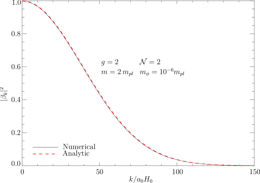
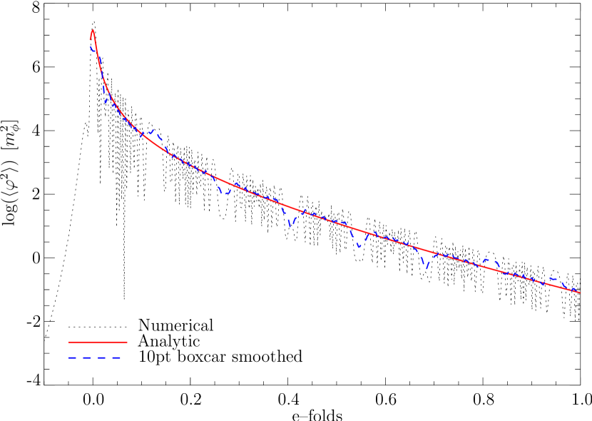
Figure 1: The number density and the time development of the correlation function, which roughly speaking is the same as the backreaction term. Both are compared to the analytic approximations, and in general there are very good agreement. The boxcar smoothing, was done to emphasise the secular evolution by canceling out the oscillations.

Comparison between the analytical approximations and numerical computation of the time evolution of the two point correlator $\langle\varphi^{2}\rangle$ has been made with excellent agreement (see figure 1). Notice in figure 1 the very steep decline in the correlation function just at the beginning. We interpret it as the first short time span, where the particles are relativistic. If we look at the approximation equation (26) for the correlation function it is singular in the beginning, because we, in making the approximation, have neglected the $k$-dependence of the energy $\omega_{k}$. Obviously we have to take that into account when $H_{0}\Delta t\ll 1$. We then find

$$\langle\varphi^{2}\rangle_{REL}\simeq\frac{1}{2\pi^{2}a^{2}}\int\rmd kk|\beta_{k}|^{2}=\frac{2n_{0}}{\sqrt{g|\dot{\phi}_{0}|}}\left(\frac{a}{a_{0}}\right)^{-2}.$$ (39)

If we now, inspired by the form of $\omega_{k}$, make an ansatz for the correlation function of the form

$$\langle\varphi^{2}\rangle=\frac{n_{0}}{g|\dot{\phi}_{0}|\sqrt{\Delta t^{2}-\Delta t^{2}_{c}}}\left(\frac{a}{a_{0}}\right)^{-3},$$ (40)

we find, by comparison with equations (26) and (39) and taking the appropriate limits, that

$$H_{0}\Delta t_{c}=\frac{H_{0}}{2\sqrt{g|\dot{\phi}_{0}|}}.$$ (41)

Equation (40) is plotted together with the numerical result in figure 1. We can interpret $H_{0}\Delta t_{c}$ as the number of e-folds where on average the energy of the produced particles is stored in relativistic modes. Because of the CMBR limit on the quadrupole, and recalling the slow-roll result, in any model of single field inflation we will have $H_{0}\Delta t_{c}\sim 10^{-3}g^{-1/2}$.

It is important to confirm the findings of [10], that the analytic approximation for the Bogoliubov coefficients is very precise. The number density $n_{k}$ is plotted in figure 1 and shows excellent agreement. Notice that at relatively high $k$-values of the wavenumber, compared to the horizon size, the number density is still significant. The energy density at the moment of particle production per logarithmic interval scales as $k^{3}n_{k}$ and therefore the peak energy occurs at values much larger than $H_{0}$. This means that the process by far and large is local in nature and the impact from the expanding background is small. It assures us that even though we have neglected all the metric backreaction terms, we still get a result which at least qualitatively agrees with what a proper treatment would yield.

In general our results for the background parameters such as the inflaton velocity and the Hubble parameter are very much in line with [10] and we will not repeat their analysis here. The reason is that the detailed evolution of the inflaton $\phi$ or the Hubble parameter $H$ do not have a direct observable impact. They would only be needed if we wanted to do a detailed analytical modelling.

2.6 The curvature perturbation

The essential quantity to consider is the comoving curvature perturbation ${\mathcal{R}}$. It is found that in the present case there is a qualitative disagreement between a numerical evaluation and any analytical prediction, regardless of whether we use the slow-roll [26], the Stewart–Lyth [27] or even the semi-numerical method of Leach et al [28]. They all disagree with our numerical approach because they assume that the impact of any change in the fields or fluctuations is local in the sense that it only affects modes which are just about to cross the horizon. However, one cannot assume the curvature perturbation to be constant on super horizon scales if the entropy perturbation is changing [21, 29], which is exactly what happens in our case. The homogeneous inflaton field suddenly dumps a large amount of energy into ultra relativistic particles. It leads to a suppression of the comoving curvature perturbation on all scales larger than the horizon, and the formation of a step in the power spectrum (see figure 2).

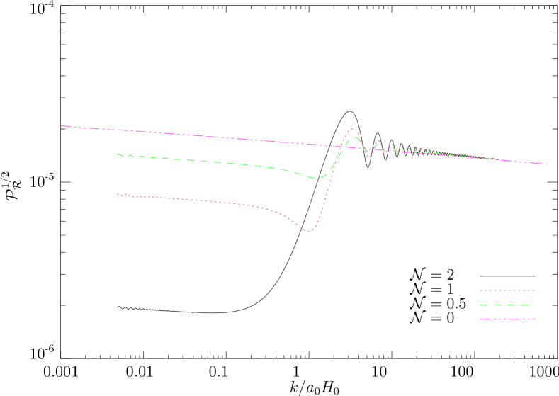
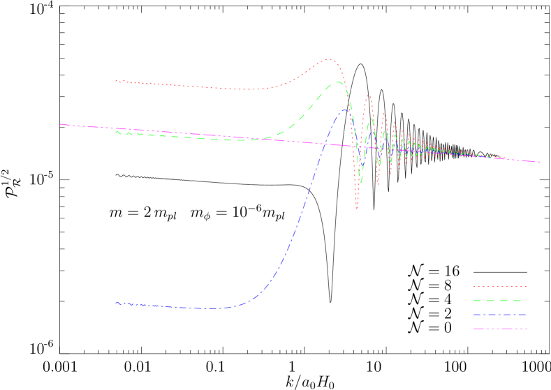
Figure 2: The power spectra from different models. In the right plot the effective number of degrees of freedom is so high that a perturbative calculation of the step height cannot be trusted, while the left plot shows the monotonic evolution of step height for weaker couplings.

On top of the main feature, the step in the potential, there are high-frequency oscillations. As is obvious from the graph the frequency increases with increasing wave number $k$. This suggests a qualitative interpretation, from a mathematical point of view, of both the step and the oscillations. The comoving curvature perturbation ${\mathcal{R}}$ is related to the inflaton field fluctuation $Q_{k}$ according to equation (7) while the power spectrum is defined in the usual way

$${\mathcal{P}}_{{\mathcal{R}}}^{1/2}=\sqrt{\frac{k^{3}}{2\pi^{2}}}\left|{\mathcal{R}}\right|.$$ (42)

To understand features in ${\mathcal{P}}_{\mathcal{R}}$ we can equally well analyse $Q_{k}$, because the change in $H$ is negligible and the change in $\dot{\phi}$ is only transient (see equation (7)).

While inside the horizon a single perturbation with definite wave number $k$ is oscillating with a frequency that is approximately given as $k/a$ (for a massless field). At the moment of particle production we can schematically write the equation for this mode $Q$ as

$$\ddot{Q}+3H\dot{Q}+\left(\frac{k^{2}}{a^{2}}+B(t)\right)Q=0,$$ (43)

where $B(t)$ is the backreaction term. Now depending on the phase of $Q$ at the exact moment of particle production the final amplitude will either be increased or decreased [30] (see second plot in figure 2). Inside the horizon the phase is highly oscillating $Q\sim\exp(-\rmi k/at)$ and we get wiggles on the UV part of the spectrum. Modes which are far outside the horizon have approximately $k/a=0$ and the amplitude changes very slowly, therefore they all experience the same kick from $B(t)$ making the step in the potential.

In the short interval, where $B^{1/2}(t)$ is greater than the Hubble mass $3/2H$, the super-horizon modes begin to oscillate again. In the perturbative regime this ‘oscillation’ lasts for such a short time that the modes do not even cross zero a single time, and we can compute the impact using simple perturbation theory. On the other hand, if $B(t)$ is large enough, zero-crossing occurs and effectively the impact from $B(t)$ is larger than the starting amplitude and perturbative methods become meaningless.

Let us define the effective step height $N_{\rm eff}$ as the quotient between the ultraviolet and the infrared part of the power spectrum ${\mathcal{P}}_{\mathcal{R}}^{1/2}$, which is the main observational signature. For small values of the coupling it is possible to make an analytic approximation for $N_{\rm eff}$. This is very valuable, because it enables us to connect the inner parameters of the theory, i.e. the coupling, the effective degrees of freedom etc, to the observable: the effective step height $N_{\rm eff}$.

For low $k$-values, until the particle production starts, $Q_{k}$ is evolving very slowly and can be taken to be constant. Then, suddenly, particle production commences. The main term in the equation of motion for $Q_{k}$ equation (27) is the two point correlation function. Define the rescaled mode $\tilde{Q}=a^{3/2}Q$ and use e-folds $N\equiv H\Delta t$ as time variable, then approximately

$$\frac{\rmd^{2}\tilde{Q}}{\rmd N^{2}}+\left(g^{2}{\mathcal{N}}\frac{\left<\varphi^{2}\right>}{H^{2}}-\frac{9}{4}\right)\tilde{Q}=0,$$ (44)

and the boundary conditions are, still for low $k$-values only,

$$\tilde{Q}(0)=\tilde{Q}_{0},\hskip 25.0pt\frac{\rmd\tilde{Q}}{\rmd N}(0)=\frac{3}{2}\tilde{Q}_{0}.$$ (45)

Unfortunately, inserting the expression equation (40) for the correlation function, we get an equation without analytical solutions. But we can exploit the fact that the integrated impact of the correlation function is supposed to be small. Then the exact functional form is not so important, only the integrated size, and instead of the correlation function can we substitute an exponential $A\rme^{-3N}$ with the correct late time behaviour. The equation can now be solved in terms of Bessel functions and plugging in the boundary conditions we get the late time behaviour and can evaluate the effective step height

$$N_{\rm eff}=1-\frac{1}{9}A+\frac{1}{324}A^{2}+\ldots.$$ (46)

$A$ can be determined by the requirement that the integrated size of the perturbation has to be the same as for the correlation function:

$$\int^{\infty}_{0}A\rme^{-3N}\rmd N=g^{2}{\mathcal{N}}\int^{\infty}_{0}\rmd N\frac{\left<\varphi^{2}\right>}{H^{2}}$$ (47)

$$A=3g^{5/2}{\mathcal{N}}\frac{\sqrt{|\dot{\phi}_{0}|}}{(2\pi)^{3}H_{0}}\left[\ln\left(\frac{2}{3H_{0}\Delta t_{c}}\right)-\gamma_{e}+3H_{0}\Delta t_{c}\right],$$

where $\gamma_{e}\simeq 0.577$ is Euler’s constant and we have evaluated the integral to first order in $H_{0}\Delta t_{c}$. The result is in agreement with the numerics.

3 Models with a changing EOS

Clearly the last section shows that the impact on the curvature perturbation on large scales is a generic feature. It has to do with the rapid change of the potential energy or, alternatively, of the equation of state. We find our result in agreement with analyses of similar models, all posessing the property of having a sudden change in the EOS.

Starobinsky [31] constructed a phenomenological model, where the potential has a break in its slope. Roberts et al [32] considered the so-called false vacuum model with quartic potential. This model is characterized by two periods, where first the potential energy is dominated by a quartic term in the inflaton, until at a certain moment a cosmological constant term takes over the leading role. In the transition period, there can be a short suspension of inflation, with related change in the EOS.

The index of EOS $\gamma$ is defined as

$$\gamma\equiv\frac{P}{\rho}=\frac{\dot{\phi}^{2}/2-V}{\dot{\phi}^{2}/2+V},$$ (48)

where we for simplicity have assumed a single-field model. The evolution equation for the $\phi$-field is a second-order equation, and it is clear that a change in the EOS can only be sourced by a change in the potential energy. In all cases $V_{\phi}$ diminishes. Because of the equation of motion

$$\ddot{\phi}+3H\dot{\phi}+V_{\phi}=0,$$ (49)

this leads to a large second-order derivative $\ddot{\phi}$ and the inflaton enters a stage of fast-roll, where approximately

$$\ddot{\phi}+3H\dot{\phi}\approx 0.$$ (50)

After some time the balance between the friction term and the source term $V_{\phi}$ is reestablished. Looking at equations (5) and (44) we can estimate that a significant change in power spectrum will only happen when

$$\frac{4V_{\phi\phi}}{9H^{2}}\geq 1,$$ (51)

for at least one e-fold. Supposing that $V_{\phi}$ during one e-fold is diminished by a factor $\epsilon$, the average change during this period is

$$\frac{\rmd V_{\phi}}{\rmd N}=-(1-\epsilon)V_{\phi}=3(1-\epsilon)H\dot{\phi}.$$ (52)

Using the last two equations we find a bound on $\epsilon$

$$\epsilon\leq{\textstyle\frac{1}{4}}.$$ (53)

It is clear that these are very rough estimates, but it does show that to get a significant change in the power spectrum of the fluctuations a rather large change in $V_{\phi}$ is required. This could either be due to interactions with other fields, as in our case, or due to the internal dynamics of the model, as in the two mentioned cases.

4 Observational data

4.1 Cosmic microwave background

The CMB temperature fluctuations are conveniently described in terms of the spherical harmonics power spectrum

$$C_{l}\equiv\langle|a_{lm}|^{2}\rangle,$$ (54)

where

$$\frac{\Delta T}{T}(\theta,\phi)=\sum_{lm}a_{lm}Y_{lm}(\theta,\phi).$$ (55)

Since Thomson scattering polarizes light, there are additional power spectra coming from the polarization anisotropies. The polarization can be divided into a curl-free $(E)$ and a curl $(B)$ component, yielding four independent power spectra: $C_{T,l}$, $C_{E,l}$, $C_{B,l}$ and the temperature $E$-polarization cross-correlation $C_{TE,l}$.

The WMAP experiment has reported data only on $C_{T,l}$ and $C_{TE,l}$, as described in [1]–[5]

We have performed the likelihood analysis using the prescription given by the WMAP collaboration which includes the correlation between different $C_{l}$s [1]–[5]. Foreground contamination has already been subtracted from their published data.

In parts of the data analysis we also add other CMB data from the compilation by Wang et al [33] which includes data at high $l$. Altogether this data set has 28 data points.

4.2 Large scale structure

The 2dF Galaxy Redshift Survey (2dFGRS) [34] has measured the redshifts of more than 230 000 galaxies with a median redshift of $z_{\rm m}\approx 0.11$. One of the main goals of the survey was to measure the galaxy power spectrum on scales up to a few hundred Mpc, thus filling in the gap between the small scales covered by earlier galaxy surveys and the largest scales where the power spectrum is constrained by observations of the CMB. A sample of the size of the 2dFGRS survey allows large-scale structure statistics to be measured with very small random errors. An initial estimate of the convolved, redshift-space power spectrum of the 2dFGRS has been determined [11] for a sample of 160 000 redshifts. On scales $0.02<k<0.15h~{}{\rm Mpc}^{-1}$ the data are robust and the shape of the power spectrum is not affected by redshift-space or nonlinear effects, though the amplitude is increased by redshift-space distortions. A potential complication is the fact that the galaxy power spectrum may be biased with respect to the matter power spectrum, i.e. light does not trace mass exactly at all scales. This is often parametrized by introducing a bias factor

$$b^{2}(k)\equiv\frac{P_{\rm g}(k)}{P_{\rm m}(k)},$$ (56)

where $P_{\rm g}(k)$ is the power spectrum of the galaxies, and $P_{\rm m}(k)$ is the matter power spectrum. Indeed it is well established that on scales less than $\sim 10~{}{\rm Mpc}$ different galaxy populations exhibit different clustering amplitudes, the so-called morphology–density relation (see e.g. [35]–[38]). Hierarchical merging scenarios also suggest a more complicated picture of biasing as it could be non-linear, scale-dependent and stochastic [39]–[44]. However, analysis of the semi-analytic galaxy formation models in [45], as well as the simulations in [43] suggest that the biasing is simple and scale-independent on large scales $k>0.15h~{}{\rm Mpc}^{-1}$ where the power spectrum is well described by linear theory, and we restrict our analysis of the 2dFGRS power spectrum to these scales. Two different analyses have demonstrated that the 2dFGRS power spectrum is consistent with linear, scale-independent bias [46, 47]. Thus, the shape of the galaxy power spectrum can be used straightforwardly to constrain the shape of the matter power spectrum on large scales.

When looking for steps or other features in the primordial power spectrum using the 2dFGRS, one should bear in mind that what is measured is the convolution of the true galaxy power spectrum with the 2dFGRS window function [11],

$$P_{\rm conv}({\bi k})\propto\int P_{\rm g}({\bi k}-{\bi q})|W_{k}({\bi q})|^{2}\rmd^{3}q,$$ (57)

where $W$ is the window function. In an earlier, simplified attempt to look for steps in the primordial power spectrum [48] it was found that the window function of the 2dFGRS more or less washed out any features in the primordial power spectrum for comoving momenta $k<0.1h~{}{\rm Mpc}^{-1}$. The effect on the class of models considered in the present paper is illustrated in figure 3 for four different values of $k_{\rm break}$. However, combining the 2dFGRS power spectrum with CMB data breaks parameter degeneracies that are present if each data set is analysed separately, and therefore a combination of large-scale structure and CMB data gives tighter constraints on the primordial power spectrum than the CMB alone.

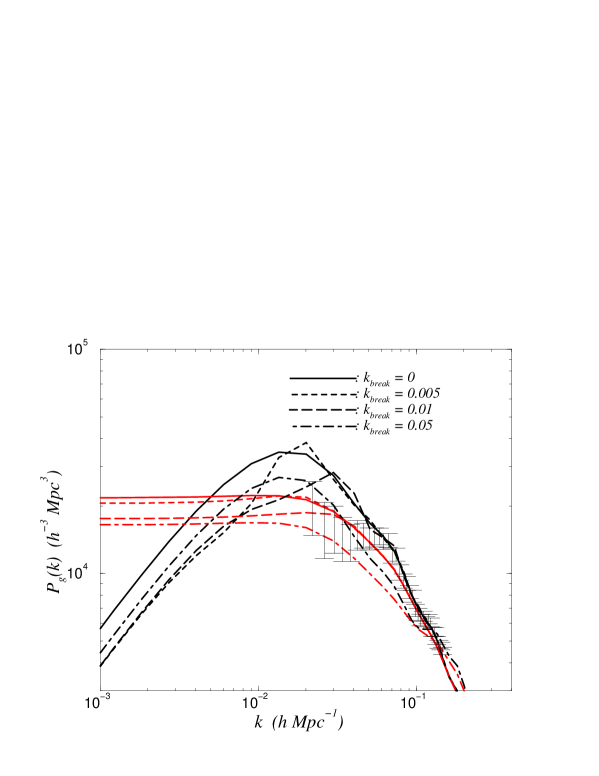
Figure 3: The effect of convolving matter power spectra with the 2dFGRS window function. The black lines are the matter power spectra computed with CMBFAST for four different values of $k_{\rm break}$, the red lines are the corresponding spectra after convolution with the window function. The vertical bars are the 2dFGRS power spectrum data points.

5 Likelihood analysis

For calculating the theoretical CMB and matter power spectra we use the publicly available CMBFAST package [49]. As the set of cosmological parameters we choose $\Omega_{m}$, the matter density, the curvature parameter, $\Omega_{b}$, the baryon density, $H_{0}$, the Hubble parameter, $n_{s}$, the scalar spectral index of the primordial fluctuation spectrum, $\tau$, the optical depth to reionization, $Q$, the normalization of the CMB power spectrum, $b$, the bias parameter, and finally the two parameters related to the step height, $N_{\rm eff}$, and location, $k_{\rm break}$. We restrict the analysis to geometrically flat models $\Omega=\Omega_{m}+\Omega_{\Lambda}=1$.

Table 1: The different priors on parameters other than $N_{\rm eff}$ and $k_{\rm break}$ used in the likelihood analysis.

Parameter	Prior
$\Omega_{m}$	$0.28\pm 0.14$ (Gaussian)
$h$	$0.72\pm 0.08$ (Gaussian)
$\Omega_{b}h^{2}$	0.014–0.040 (top hat)
$n$	0.6–1.4 (top hat)
$\tau$	0–1 (top hat)
$Q$	free
$b$	free

In principle one might include even more parameters in the analysis, such as $r$, the tensor to scalar ratio of primordial fluctuations. However, $r$ is most likely so close to zero that only future high precision experiments may be able to measure it. The same is true for other additional parameters. Small deviations from slow-roll during inflation can show up as a logarithmic correction to a simple power-law spectrum [50]–[52], or additional relativistic energy density [53]–[61] could be present. However, there is no evidence of any such effect in the present data and therefore we restrict the analysis to the ‘minimal’ standard cosmological model.

In this full numerical likelihood analysis we use the free parameters discussed above with certain priors (see table 1) determined from cosmological observations other than CMB and LSS. In flat models the matter density is restricted by observations of Type Ia supernovae to be $\Omega_{m}=0.28\pm 0.14$ [62]. The current estimated range for $\Omega_{b}h^{2}$ from BBN is $\Omega_{b}h^{2}=0.020\pm 0.002$ [63], and finally the HST Hubble key project has obtained a constraint on $H_{0}$ of $72\pm 8~{}{\rm km}~{}{\rm s}^{-1}~{}{\rm Mpc}^{-1}$ [64]. The actual maginalization over parameters other than $N_{\rm eff}$ and $k_{\rm break}$ was performed using a simulated annealing procedure [65].

In figure 4 we show results of the likelihood calculation for various different data sets. In panel (a) results are shown for an analysis with all available data, WMAP, the Wang et al compilation and the 2dFGRS power spectrum. In panel (b) we show results for WMAP + Wang, in panel (c) for WMAP + 2dFGRS, and finally in panel (d) for WMAP data only. The figure shows the 68% and 95% exclusion limits for the parameters $N_{\rm eff}$ and $k_{\rm break}$. These two contours correspond to $\Delta\chi^{2}=2.31$ and $\Delta\chi^{2}=6.17$ respectively. Best fit values and number of degrees of freedom for each of the four cases are listed in table 2.

Figure 4: 68% and 95% confidence exclusion plot of the parameters $N_{\rm eff}$ and $k_{\rm break}$ for the four different cases described in the text. The horizontal lines show the range in $k$-space covered by various data sets. CMB data have been converted from $k$ to $l$ using the approximate prescription $l\simeq 2k/H_{0}$.

Several things can be noted from this figure. First, the 2dFGRS power spectrum only constrains a step-like feature on scales smaller than $k\sim 0.05-0.1h~{}{\rm Mpc}^{-1}$ because the window function of the survey washes out any features on scales larger than this.

Second, the CMB data are mainly sensitive to scales corresponding to $l\sim 50$–100, and only to a lesser extent to features at high $l$. The main reason for this is that CMB data do not directly probe the primordial power spectrum, but rather the primordial spectrum convolved with an effective window function. This will be discussed in detail in the next subsection. The result of the convolution is that a sharp step in $P(k)$ appears as a gradual increase in power over a range in $l$ in the CMB spectrum. It is relatively easy to mask this effect by changing other cosmological parameters. However, scales at $l\,\hbox to0.0pt{\lower 3.5pt\hbox{$\mathchar 0\relax\sim$}\hss}\raise 1.0pt\hbox{$<$}\,100$ were outside the particle horizon at recombination and therefore much less sensitive to changes in most of the cosmological parameters. This is the reason why the likelihood analysis shows a very stringent bound in this range, and not in the region around the first acoustic peak, as could perhaps have been expected.

Table 2: Best fit $\chi^{2}$ and number of degrees of freedom for each of the cases shown in figure 4.

Case	$\chi^{2}$	d.o.f.	$\chi^{2}$/d.o.f.
(a)	1466.9	1388	1.057
(b)	1459.2	1371	1.064
(c)	1440.9	1360	1.059
(d)	1432.2	1343	1.065

Finally, adding the Wang et al compilation to the WMAP data significantly tightens the bound on $N_{\rm eff}$ over most of the range in $k$-space, particularly of course at the smaller scales where the WMAP data suffer from finite angular resolution. However, in some parts of parameter space the constraint actually becomes slightly worse by adding other CMB data. This is not inconsistent, it just means that the Wang et al data actually favour a small step and therefore push the total likelihood towards higher values of $N_{\rm eff}$.

In the last panel the effect of the final resolution of the WMAP data becomes apparent beyond $k\sim 0.05h~{}{\rm Mpc}^{-1}$, corresponding to $l\sim 450$, exactly around the scale where the error bars are no longer cosmic variance limited.

Finally, we note that our analysis is restricted to geometrically flat models. However, since spatial geometry affects the CMB spectrum at scales $l\,\hbox to0.0pt{\lower 3.5pt\hbox{$\mathchar 0\relax\sim$}\hss}\raise 1.0pt\hbox{$<$}\,100$ it is possible that the accuracy with which we have constrained $N_{\rm eff}$ on this scale has been slightly overestimated.

5.1 The CMB window function

CMB data do not directly measure the underlying primordial power spectrum of fluctuations. Rather, they measure the spectrum folded with a transfer function in the following sense

$$C_{l}=\int\frac{\rmd k}{k}P(k)\Delta_{l}^{2}(k),$$ (58)

where $\Delta_{l}^{2}(k)$ is the transfer function taken at the present, $\tau=\tau_{0}$, and $\tau$ is conformal time. Following the line-of-sight approach pioneered by Seljak and Zaldariagga [49] this transfer function can be written as

$$\Delta(k)=\int_{0}^{\tau_{0}}\rmd\tau S(k,\tau)j_{l}[k(\tau-\tau_{0})],$$ (59)

where $S$ is a source function, calculated from the Boltzmann equation, and $j_{l}(x)$ is a spherical Bessel function. However, in order to get a very rough idea about the effective window function $w_{l}(k)=\Delta_{l}^{2}(k)/k$ of the CMB we approximate $S$ with a constant to obtain

$$w_{l}(k)\propto\cases{\left(\frac{k\tau_{0}}{l}\right)^{l}\sim 0&for $k\tau_{0}\,\hbox to0.0pt{\lower 3.5pt\hbox{$\mathchar 0\relax\sim$}\hss}\raise 1.0pt\hbox{$<$}\,l$\cr\frac{1}{k^{3}}&for $k\tau_{0}\,\hbox to0.0pt{\lower 3.5pt\hbox{$\mathchar 0\relax\sim$}\hss}\raise 1.0pt\hbox{$>$}\,l$.}$$ (60)

This simple equation shows several things: (a) A feature at some specific wavenumber $k=k_{*}$ has the greatest impact on the CMB spectrum at $l_{*}\simeq k_{*}\tau_{0}$. For a flat, matter dominated universe, $\tau_{0}=2/H_{0}$, yielding $l_{*}\simeq 2k_{*}/H_{0}$. (b) The CMB window function is quite broad, and narrow features in $P(k)$ are accordingly difficult to detect.

In the present model the main detectable feature is a step in the power spectrum, characterized by the amplitude, $N_{\rm eff}$, and the location, $k_{\rm break}$. Adding such a step to an otherwise scale-invariant spectrum yields a primordial power spectrum

$$P(k)=A+N_{\rm eff}\Theta(k-k_{\rm break}).$$ (61)

Calculating $C_{l}$ from equation (58), using the window function equation (60) then gives us

$$C_{l}\propto\cases{\frac{A+N_{\rm eff}}{(l/\tau_{0})^{2}}&for $k_{\rm break}\tau_{0}\,\hbox to0.0pt{\lower 3.5pt\hbox{$\mathchar 0\relax\sim$}\hss}\raise 1.0pt\hbox{$<$}\,l$\\ \frac{A}{(l/\tau_{0})^{2}}+\frac{N_{\rm eff}}{k^{2}_{\rm break}}&for $k_{\rm break}\tau_{0}\,\hbox to0.0pt{\lower 3.5pt\hbox{$\mathchar 0\relax\sim$}\hss}\raise 1.0pt\hbox{$>$}\,l$.}$$ (62)

Finally, we can define the ratio, $R$, between the CMB spectrum with the step, and one with exactly the same cosmological parameters, but without the step

$$R=\cases{1+\frac{N_{\rm eff}}{A}&for $k_{\rm break}\tau_{0}\,\hbox to0.0pt{\lower 3.5pt\hbox{$\mathchar 0\relax\sim$}\hss}\raise 1.0pt\hbox{$<$}\,l$\\ 1+\frac{N_{\rm eff}}{A}\left(\frac{l}{k_{\rm break}\tau_{0}}\right)^{2}&for $k_{\rm break}\tau_{0}\,\hbox to0.0pt{\lower 3.5pt\hbox{$\mathchar 0\relax\sim$}\hss}\raise 1.0pt\hbox{$>$}\,l$.}$$ (63)

Figure 5: Ratio of $C_{l}$ for model with step to model without step. The full line is the precise numerical calculation and the dashed is the approximation in Eq. (63).

In figure 5 we show the ratio of two spectra calculated with CMBFAST. The first model is a standard $\Omega_{m}=1$ CDM model with $h=0.7$ and scale-invariant initial spectrum, $P(k)=A$. The second model is with the same parameters, but with a step added, with parameters $N_{\rm eff}=A$ and $k_{\rm break}=0.05$ Mpc^-1. The full line shows the numerical result, and the dashed line shows the approximation from equation (63). Clearly our very simple approximation still captures the essential impact of a step-like feature on the CMB spectrum. The reason for choosing a CDM model, rather than the observationally preferred $\Lambda$CDM concordance model, is simply that in the former case $\tau_{0}=2H_{0}^{-1}$, making the analytic expression in equation (63) particularly simple. Using the $\Lambda$CDM model as the benchmark yields almost exactly the same result.

The conclusion is that the effective window function $w_{l}(k)$ for CMB smooths out the step feature in the underlying primordial power spectrum $P(k)$. This in turn means that the ability of CMB data to detect step-like features is significantly degraded.

A feature which is at first surprising is that the constraint on the step amplitude $N_{\rm eff}$ is strongest at $k_{\rm break}\sim 0.01$, corresponding to $l\sim 90$ which is significantly above the scale of the first acoustic peak. The reason is that scales above $l\sim 100$ were outside the particle horizon at recombination and therefore the CMB spectrum at these scales is not susceptible to acoustic oscillation effects which can otherwise mask a step in the primordial spectrum. At $l\,\hbox to0.0pt{\lower 3.5pt\hbox{$\mathchar 0\relax\sim$}\hss}\raise 1.0pt\hbox{$<$}\,30$ the constraint on $N_{\rm eff}$ becomes gradually weaker simply because cosmic variance increases the error bars on $C_{l}$. Clearly, even though the present CMB data are most sensitive to step features at scales corresponding to $l\sim 50$–100 a future experiment like Planck which is cosmic variance limited out to $l\,\hbox to0.0pt{\lower 3.5pt\hbox{$\mathchar 0\relax\sim$}\hss}\raise 1.0pt\hbox{$>$}\,2000$ would be able to put strong constraints on $N_{\rm eff}$ at much higher $l$, simply because the greater measurement accuracy would break the degeneracy between a step and changes in other cosmological parameters.

6 Discussion

We have presented a calculation of the perturbation to the power spectrum that is generated under inflation due to a resonant coupling of the inflaton to a boson. The calculation has been made only under the assumption of slow-roll evolution of the inflaton before and after the interaction, but no constraints have been put on the specific form of the potential. In [10] the same setup was studied, but with a trilinear coupling to a fermion field. Our results for the perturbation to the primordial power spectrum are dramatically different to their findings. A step-like feature is formed, and on top of this, to the ultraviolet side of the step, there is a highly oscillating transient. For weak couplings the size of the step scales like $g^{5/2}{\mathcal{N}}$ and a suppression of power on large scales is observed, while at larger values of the coupling and the dengeneracy this simple relation breaks down and suppression or enhancement of the large scale power relative to the ultraviolet part can occur (see figure 2).

The differences we observe with respect to the results of Chung et al [10] are easily explained from the more limited analysis they performed. Indeed similar numerical studies support our conclusion. Easther et al [30] have investigated the impact from a step in the potential of the inflaton and found a very similar feature. They reproduce the oscillations seen in our model, but no significant amplification is observed. Leach et al undertook a detailed investigation of the false vacuum model [66] where they found a suppression of the infrared part of the spectrum caused by changes in the entropy perturbation very much like the one we observe. Starobinsky [31] explored the very simplest model, where the inflationary potential has a step, and reached the same conclusion. Common for all studies is that the effects seen are due to the self contained dynamics of the field, while in our model they are caused by the mutual interaction between the inflaton and external fields. This is a major difference, and while the other models require fine tuning of the potential, such that the ‘feature’ occurs in the small range accessible to observational cosmology, our model can be naturally supported in the context of supersymmetric theories with extra dimensions or superstring theories. These theories can have a whole hierarchy of particles with masses comparable to the Planck mass [10, 67, 68]. It would then be much more natural to expect at least one particle with parameters, such that the produced feature falls into the range open to observations [8]. Nonetheless, the presented model should be understood as a realistic toy model, while a real model should have some basis in particle physics.

It would have been desirable to do a full numerical study including higher order metric terms coming from the gravitational interaction of the fields. We think, though, that the overall features of the phenomena are correctly described in this analysis. It can be argued, that because the particles are produced relativistically and the peak wave number is very large in comparison with the Hubble horizon at that epoch, the process should be causal in nature, and therefore not much dependent on the expansion of the universe.

One feature we did miss in our study, which could be important, is the quantum treatment of the inflaton fluctuations and the possibility of cross correlations between the fields. The step feature is largely due to the backreaction of the coupled particle directly on the inflaton fluctuations, and therefore the cross correlation could be almost maximal. This leads to the possibility, that some of the energy contained in the inflaton fluctuations oscillates into fluctuations in the other species and is redshifted away [69]. This clearly has to be addressed in a future study.

Using the recently published WMAP data together with other CMB data compiled by Wang et al and large scale data from the 2DF collaboration we have found new upper limits on a break in the primordial power spectrum. We did the full likelihood analysis, and our conclusions are robust: the derived limits changed only slightly while varying the amount of data put into the analysis. We find that on scales corresponding to $k\sim 0.001$–$0.03h~{}{\rm Mpc}^{-1}$ the $2\sigma$ upper limit on $N_{\rm eff}$—the relative step height—is $\sim 0.3$. This conclusion is not sensitive to the chosen compilation of data and can essentially be derived from the WMAP data only. We also note that the CMB spectrum is mainly sensitive to features at scales corresponding to $l\sim 50$–100 and only to a lesser extent features at high $l$. This is because scales corresponding to $l\,\hbox to0.0pt{\lower 3.5pt\hbox{$\mathchar 0\relax\sim$}\hss}\raise 1.0pt\hbox{$<$}\,100$ were outside the particle horizon at recombination and much less affected by changes in most of the cosmological parameters. The constraint is significantly strengthened around $l\sim 100$ by adding other data than WMAP. This is indirectly through their tightening of the limits on the cosmological parameters translating into less freedom to cancel the effect of a break around $l\sim 50$–100. While observations of the CMB give us a wonderful tool to constrain the cosmology of our universe there is no a priori reason to expect a smooth almost scale invariant power spectrum. The possibility of inherent noise and deviations in the primordial power spectrum gives us a promising prospect to probe the earliest history of our universe, but also have the potential of fooling cosmological parameter estimation at the per cent level. One should remember this extra uncertainty of ‘unknown physics’, when reading about limits set by new experiments. While so far there has been no trace of it, the deviation from full scale invariance and a possible bend in the power spectrum, as has been inferred by the WMAP team using their data, the 2DF survey and Lyman-alpha forest data, tells us that we are reaching levels of precision, where features could begin to crystalize out from the experimental errors.

It should be noted that our likelihood analysis for $k_{\rm break}$ and $N_{\rm eff}$ is in fact quite general and can be applied to other models which produce a break in the power spectrum. Of course the oscillating behaviour of the spectrum close to the break is very specific to the present model, but the width of the window functions for both CMB and LSS tends to blur the oscillations so that the observational constraints are essentially on the step height and position.

Our result for $(k_{\rm break},N_{\rm eff})$ can therefore be compared for instance to the study of [70]. In that study it was found that the WMAP data show a slight preference for a step in the power spectrum at $k\simeq 2$–$3\times 10^{-4}$ Mpc^-1. In their analysis it was assumed that there was no power above the step scale, which in our language corresponds to $N_{\rm eff}\to\infty$. In fact our WMAP-only analysis shows that the region where $N_{\rm eff}\to\infty$ and $k_{\rm break}\simeq 1.5$–$2.5\times 10^{-4}$ Mpc^-1 provides a slightly better fit than no break. However, we find that this effect is not statistically significant.

Finally we note that our study only probes the scales measurable by CMB and LSS experiments. On much smaller scales limits on primordial black holes provide tight constraints on the primordial power spectrum (see for instance [71]) and can therefore be expected to provide interesting constraints on step-like features, limiting theories predicting the occurence of particle production and phase transitions on a much wider range of scales.

References

References

- [1] Bennett C L et al, 2003 Preprint astro-ph/0302207
- [2] Spergel D N et al, 2003 Preprint astro-ph/0302209
- [3] Kogut A et al, 2003 Preprint astro-ph/0302213
- [4] Hinshaw G et al, 2003 Preprint astro-ph/0302217
- [5] Verde L et al, 2003 Preprint astro-ph/0302218
- [6] Peiris H et al, 2003 Preprint astro-ph/0302225
- [7] La D and Steinhardt P J, Phys. Rev. Lett. 62, 376 (1989)
- [8] Adams J A, Ross G G, and Sarkar S, Nucl. Phys. B 503, 1997 (405)
- [9] Starobinsky A A, Grav. Cosmol. 4, 88 (1998)
- [10] Chung D J H, Kolb E W, Riotto A and Tkachev I I, Probing Planckian physics: resonant production of particles during inflation and features in the primordial power spectrum, Phys. Rev. D62 043508 2000, [ hep-ph/9910437]
- [11] Percival W J et al (the 2dFGRS team), 2001 Mon. Not. R. Astron. Soc. 327 1297
- [12] Kofman L, Linde A and Starobinsky A A, Towards the theory of reheating after inflation, Phys. Rev. D56 3258-3295 1997, [hep-ph/9704452].
- [13] Birrell N D and Davies P C W, 1982 Quantum Fields in curved space time (Cambridge: Cambridge University Press)
- [14] Cormier D, Heitmann K and Mazumdar A, Dynamics of coupled bosonic systems with applications to preheating, 2001 Preprint [hep-ph/0105236]
- [15] Baacke J, Heitmann K and Patzold C, Nonequilibrium dynamics of fermions in a spatially homogeneous scalar background field, 1998 Phys. Rev. D 58 125013 [hep-ph/9806205]
- [16] Baacke J and Patzold C, Renormalization of the nonequilibrium dynamics of fermions in a flat FRW universe, 2000 Phys. Rev. D 62 084008 [hep-ph/9912505]
- [17] Mukhanov V F, Feldman H A and Brandenberger R H, Theory of cosmological perturbations. Part 1: Classical perturbations. Part 2: Quantum theory of perturbations. Part 3: Extensions, 1992 Phys. Rept. 215, 203-333
- [18] Abramo L R W, The back reaction of gravitational perturbations and applications in cosmology, 1997 Preprint gr-qc/9709049
- [19] Bruni M, Matarrese S, Mollerach S and Sonego S, Perturbations of spacetime: gauge transformations and gauge invariance at second order and beyond, Class. Quant. Grav. 14, 1997 (2585) [gr-qc/9609040]
- [20] Gordon C, Wands D, Bassett B A and Maartens R, Adiabatic and entropy perturbations from inflation, 2001 Phys. Rev. D 63 023506 [astro-ph/0009131]
- [21] Wands D, Malik K A, Lyth D H and Liddle A R, A new approach to the evolution of cosmological perturbations on large scales, 2000 Phys. Rev. D 62 043527 [astro-ph/0003278]
- [22] Liddle A R, Lyth D H, Malik K A and Wands D, 2000 Phys. Rev. D 61 103509 [hep-ph/9912473]
- [23] Acquaviva V, Bartolo N, Matarrese S and Riotto A, 2002 Preprint astro-ph/0209156
- [24] Maldecena J, Non-Gaussian features of primordial fluctuations in single field inflatio nary models, JHEP05(2003)013 [astro-ph/0210603]
- [25] Rigopoulos G, 2002 Preprint astro-ph/0212141
- [26] Abbott L F and Wise M B, Constraints on generalized inflationary cosmologies, Nucl. Phys. B 244, 1984 (541)
- [27] Stewart E D and Lyth D H, A More accurate analytic calculation of the spectrum of cosmological perturbations produced during inflation, Phys. Lett. B 302, 1993 (171) [gr-qc/9302019]
- [28] Leach S M, Sasaki M, Wands D and Liddle A R, Enhancement of superhorizon scale inflationary curvature perturbations, 2001 Phys. Rev. D 64 023512 [astro-ph/0101406]
- [29] Wands D, 2002 Preprint astro-ph/0201541 Malik K, Wands D and Ungarelli C, 2002 Preprint astro-ph/0211602 Di Marco F, Finelli F and Brandenberger R, 2002 Preprint astro-ph/0211276
- [30] Adams J, Cresswell B and Easther R, Inflationary perturbations from a potential with a step, 2001 Preprint astro-ph/0102236
- [31] Starobinsky A A, 1985 Sov. Phys. JETP Lett. 42, 51
- [32] Roberts D, Liddle A R and Lyth D H, False vacuum inflation with a quartic potential, 1995 Phys. Rev. D 51 4122 [astro-ph/9411104]
- [33] Wang X, Tegmark M, Jain B and Zaldarriaga M, The last stand before MAP: cosmological parameters from lensing, CMB and galaxy clustering, 2002 Preprint astro-ph/0212417
- [34] Colless M et al (the 2dFGRS team), 2001 Mon. Not. R. Astron. Soc. 328 1039
- [35] Dressler A, Galaxy morphology in rich clusters—implications for the formation and evolution of galaxies, 1980 Astrophys. J. 236 351
- [36] Hermit S, Santiago B X, Lahav O, Strauss M A, Davis M, Dressler A and Huchra J P, The two-point correlation function and morphological seggregation in the Optical Redshift Survey, 1996 Mon. Not. R. Astron. Soc. 283 709 [astro-ph/9608001]
- [37] Norberg P et al (the 2dFGRS team), The 2dF Galaxy Redshift Survey: the dependence of galaxy clustering on luminosity and spectral type, 2002 Mon. Not. R. Astron. Soc. 332 827 [astro-ph/0112043]
- [38] Zehavi I et al (SDSS Collaboration), Galaxy clustering in early Sloan Digital Sky Survey Redshift data, 2002 Astrophys. J. 571 172 [astro-ph/0106476]
- [39] Mo H J and White S D M, An analytic model for the spatial clustering of dark matter haloes, 1996 Mon. Not. R. Astron. Soc. 282 347 [astro-ph/9512127]
- [40] Matarrese S, Coles P, Lucchin F and Moscardini L, Redshift evolution of clustering, 1997 Mon. Not. R. Astron. Soc. 286 115 [astro-ph/9608004]
- [41] Magliochetti M, Bagla J, Maddox S J and Lahav O, The observed evolution of galaxy clustering vs. epoch-dependent biasing models, 2000 Mon. Not. R. Astron. Soc. 314 546 [astro-ph/9902260]
- [42] Dekel A and Lahav O, Stochastic nonlinear galaxy biasing, 1999 Astrophys. J. 520 24 [astro-ph/9806193]
- [43] Blanton M, Cen R, Ostriker J P, Strauss M A and Tegmark M, Time evolution of galaxy formatino and bias in cosmological simulations, 2000 Astrophys. J. 531 1 [astro-ph/9903165]
- [44] Somerville R, Lemson G, Sigad Y, Dekel A, Colberg J, Kauffmann G and White S D M, Non-linear stochastic galaxy biasing in cosmological simulations, 2001 Mon. Not. R. Astron. Soc. 320 289 [astro-ph/9912073]
- [45] Berlind A A, Weinberg D H, Benson A J, Baugh C M, Cole S, Davé R, Frenk C S, Katz N and Lacey C G, The halo occupation distribution and the physics of galaxy formation, 2002 Preprint astro-ph/0212357
- [46] Lahav O et al (the 2dFGRS team), 2002 Mon. Not. R. Astron. Soc. 333 961
- [47] Verde L et al (the 2dFGRS team), 2002 Mon. Not. R. Astron. Soc. 335 432
- [48] Elgarøy Ø, Gramann M and Lahav O, Features in the primordial power spectrum: constraints from the cosmic microwave background and the limitation of the 2dF and SDSS redshift surveys to detect them, 2002 Mon. Not. R. Astron. Soc. 333 93 [astro-ph/0111208]
- [49] Seljak U and Zaldarriaga M, 1996 Astrophys. J. 469 437
- [50] Hannestad S, Hansen S H and Villante F L, Probing the power spectrum bend with recent CMB data, 2001 Astropart. Phys. 16 137 [astro-ph/0012009]
- [51] Hannestad S, Hansen S H, Villante F L and Hamilton A J, Constraints on inflation from CMB and Lyman-alpha forest, 2002 Astropart. Phys. 17 375 [astro-ph/0103047]
- [52] Griffiths L M, Silk J and Zaroubi S, 2000 Preprint astro-ph/0010571
- [53] Jungman G, Kamionkowski M, Kosowsky A and Spergel D N, Cosmological parameter determination with microwave background maps, 1996 Phys. Rev. D 54 1332 [astro-ph/9512139]
- [54] Lesgourgues J and Peloso M, Remarks on the Boomerang results, the cosmological constant and the leptonic asymmetry, 2000 Phys. Rev. D 62 081301 [astro-ph/0004412]
- [55] Hannestad S, New constraints on neutrino physics from Boomerang data, 2000 Phys. Rev. Lett. 85 4203 [astro-ph/0005018]
- [56] Esposito S, Mangano G, Melchiorri A, Miele G and Pisanti O, Testing standard and degenerate big bang nucleosynthesis with BOOMERanG and MAXIMA-1, 2001 Phys. Rev. D 63 043004 [astro-ph/0007419]
- [57] Kneller J P, Scherrer R J, Steigman G and Walker T P, When does CMB + BBN = new physics?, 2001 Phys. Rev. D 64 123506 [astro-ph/0101386]
- [58] Hannestad S, New CMBR data and the cosmic neutrino background, 2001 Phys. Rev. D 64 083002 [astro-ph/0105220]
- [59] Hansen S H, Mangano G, Melchiorri A, Miele G and Pisanti O, Constraining neutrino physics with BBN and CMBR, 2002 Phys. Rev. D 65 023511 [astro-ph/0105385]
- [60] Bowen R, Hansen S H, Melchiorri A, Silk J and Trotta R, The impact of an extra background of relativistic particles on the cosmological parameters derived from microwave background anisotropies, 2001 Preprint astro-ph/0110636
- [61] Dolgov A D, Hansen S H, Pastor S, Petcov S T, Raffelt G G and Semikoz D V, Cosmological bounds on neutrino degeneracy improved by flavor oscillations, 2002 Preprint hep-ph/0201287
- [62] Perlmutter S et al (Supernova Cosmology Project Collaboration), Measurements of Omega and Lambda from 42 high-redshift supernovae, 1999 Astrophys. J. 517 565 [astro-ph/9812133]
- [63] Burles S, Nollett K M and Turner M S, Big-bang nucleosynthesis predictions for precision cosmology, 2001 Astrophys. J. 552 L1 [astro-ph/0010171] See also Olive K A, Steigman G and Walker T P, Primordial nucleosynthesis: Theory and observations, 2000 Phys. Rept. 333 389 for a recent review [astro-ph/9905320]
- [64] Freedman W L et al, 2001 Astrophys. J. 553 L47
- [65] Hannestad S, Stochastic optimization methods for extracting cosmological parameters from cosmic microwave background radiation power spectra, 2000 Phys. Rev. D 61 023002
- [66] Leach S M and Liddle A R, Inflationary perturbations near horizon crossing, 2001 Phys. Rev. D 63 043580 [astro-ph/0010082]
- [67] Lyth D H and Riotto A, Particle physics models of inflation and the cosmological density perturbation, 1999 Phys. Rept. 314 1 [hep-ph/9807278]
- [68] Malik K A, Cosmological perturbations in an inflationary universe, 2001 Preprint astro-ph/0101563
- [69] Bartolo N, Matarrese S and Riotto A, Oscillations during inflation and cosmological density perturbations, 2001 Phys. Rev. D 64 083514 [astro-ph/0106022]
- [70] Bridle S L, Lewis A M, Weller J and Efstathiou G, Reconstructing the primordial power spectrum, 2003 Preprint astro-ph/0302306
- [71] Bringmann T, Kiefer C and Polarski D, Primordial black holes from inflationary models with and without broken scale invariance, 2002 Phys. Rev. D 65 024008 [astro-ph/0109404]