Gravitation in the fractal $D=2$ inertial universe:
New phenomenology in spiral discs and a
theoretical basis for MOND

Abstract

A particular interpretation of Mach’s Principle led us to consider if it was possible to have a globally inertial universe that was irreducibly associated with a non-trivial global matter distribution, Roscoe [$2002$a]. This question received a positive answer, subject to the condition that the global matter distribution is necessarily fractal, $D=2$. The purpose of the present paper is to show how general gravitational processes arise in this universe. We begin by showing how classical Newtonian gravitational processes arise from point-source perturbations of this $D=2$ inertial background. We are then able to use the insights gained from this initial analysis to arrive at a general theory for arbitrary material distributions. We illustrate the process by using it to model an idealized spiral galaxy. One particular subclass of solutions, corresponding to logarithmic spirals, has already been extensively tested (Roscoe [1999a], [$2002$b]), and shown to resolve dynamical data over large samples of optical rotation curves (ORCs) with a very high degree of statistical precision.

Whilst the primary purpose of the data analysis of Roscoe [1999a] was to test the predictions of the logarithmic spiral theory, it led directly to the discovery of a major new phenomenology in spiral discs - that of discrete dynamical classes - initially reported in Roscoe [1999b] and comprehensively confirmed in Roscoe [$2002$b] over four large independent samples of ORCs. In this paper, we analyse the theory more comprehensively, and show how the discrete dynamical classes phenomenology has a ready explanation in terms of an algebraic consistency condition which must necessarily be satisfied.

Of equal significance, we apply the theory with complete success to the detailed modelling of a sample of eight Low Surface Brightness spirals (LSBs) which, hitherto, have been succesfully modelled only by the MOND algorithm (Modified Newtonian Dynamics, Milgrom [1983a], [1983b], [1983c]). The CDM models have failed comprehensively when applied to LSBs. We are able to conclude that the essence of the MOND algorithm must be contained within the presented theory.

Mach – Spiral Galaxy – Rotation Curve – MOND – Gravitation

1 Introduction

1.1 Review of Preliminary Work:

General Relativity can be considered as a theory of what happens to predetermined clocks and rods in the presence of material systems (material here is understood in its widest sense). By contrast, the theory being discussed here can be considered as a primitive, but fundamental, theory of how clocks and rods arise in the first place within material systems.

The preliminary work (Roscoe [$2002$a]) was driven by the idea that it is impossible to conceive of physical (metric) space in the absence of material systems, and that it is similarly impossible to conceive of physical time in the absence of process within these material systems. Following upon this, we took the point of view that any fundamental theory of space & time must then necessarily have the property that, within it, it is impossible to talk about metrical space & physical time in the absence of any material system. In effect, this is the view that notions of material systems are logically prior to notions of clocks & rods, and that these latter notions are somehow projected out of prior relations which exists between the individual elements which make up the former.

We began by noting that the most simple form of space & time we can conceive is that of inertial space & time - that is, a space & time within which the relations between clocks and rods are fixed. And then, keeping to the spirit of the basic idea, we posed the questions:

• Can a globally inertial space & time be associated with a non-trivial global matter distribution ?

• And, if so, what are the general properties of this distribution ?

These questions were addressed within the context of an extremely simple model universe populated by particles which possessed only the property of enumerability, and within which there were no predetermined ideas of clocks & rods. It was required that these concepts should emerge from the general analysis. To simplify the initial development, it was originally assumed that the model universe was stationary. It transpired that this assumption was equivalent to choosing a one-clock quasi-classical model, whilst relaxing the assumption was equivalent to choosing a two-clock relativistic model. The work of this paper is based upon the one-clock quasi-classical development.

The original questions were then answered as follows: a globally inertial space & time can be associated with a non-trivial matter distribution, and this distribution is necessarily fractal $D=2$. However, it transpires that the particles in this matter distribution cannot reasonably be identified with ordinary matter since (in crude terms) the particles all appear to be in states of randomly directed uniform motion, but with identical speeds of magnitude $v_{0}$. In other words, the distribution has some of the attributes of a quasi-photon gas and, for this reason, we interpreted it as a rudimentary model of a material vacuum. A closer investigation then shows that, in fact, whilst $v_{0}$ has the dimensions of speed, it is more properly interpreted as a conversion factor between length scales and temporal scales - in this sense, $v_{0}$ is more like Bondi’s interpretation of $c$. It follows from this that the material vacuum itself appears to have the role of arbitrating between length scales and temporal scales.

We then noted that, if ordinary matter could, somehow, condense out of this $D=2$ material vacuum then we would have a universe of ordinary matter which is in close accord with what is actually observed in galaxy counts out to medium distances - that is, on these medium scales, the material distribution in the form of galaxies has vanishingly small accelerations and is distributed in a quasi-fractal form with $D\approx 2$.

1.2 The Emergence of Gravitation

Once one has a particular conception of ‘inertial space & time’ (for example, that of Newtonian theory, or that of Einstein’s special relativity), a theory of gravitation effectively follows as a perturbation of that particular inertial space & time.

For example, in the Newtonian context, such perturbations are interpreted as the introduction of gravitational forces into a previously force-free environment whilst, in the Einsteinien case, they are interpreted as the introduction of curvature into a flat spacetime manifold. In the present case, they are literally perturbations of the $D=2$ distribution of material in the rudimentary model vacuum. Since the $D=2$ distribution is irreducibly associated with clocks & rods in a fixed relationship with each other, it follows that any perturbation from $D=2$ will necessarily entail distortions of the clocks & rods relationship, and will therefore give rise to what are conventionally called gravitational processes.

1.3 Qualitative Gravitational Mechanisms

Newton introduced the idea of force into discourse about the world through his mechanics, and his Law of Gravitation can be viewed as a recipe quantifying the amount of force acting between two massive bodies. However, Newton famously said that he had no idea what constituted the fundamental essence of this gravitational force and today, the whole theory is simply accepted as an enormously successful and useful means of describing the phenomenology.

Exactly the same can be said of General Relativity: that is, gravitational processes are said to arise in this theory when the flat spacetime manifold becomes curved by the presence of mass. The field equations can be viewed simply as the recipe which quantifies the amount of curvature created by a given distribution of mass. But, as with Newtonian theory, the mechanism by which this is achieved is absent. So, at one level, General Relativity can be considered as simply an alternative means of describing the phenomenology - albeit one which applies in far more extreme circumstances.

The case of the present theory is different: the search for a gravitational mechanism was emphatically not part of our original thinking and, in the main body of this paper, we pay no attention at all to the likely nature of any such mechanism. We simply perform a formal perturbation analysis of the $D=2$ inertial universe, and the analysis is played out geometrically on a curved manifold using largely familiar techniques. However, regardless of this, it is impossible not to realize that a genuine mechanism has automatically presented itself. Specifically, we have mentioned that the material in the idealized $D=2$ inertial universe behaves like a quasi-photon gas, and that gravitational processes arise when this $D=2$ distribution is perturbed - in particular, point-wise spherically symmetric perturbations are interpreted as being due to the presence of conventional point masses. One is then immediately forced to conclude that the point-mass perturbs by acting as either a source or a sink of quasi-photon gas. Suppose it is a sink, and that its mass simply quantifies the amount of absorption going on; then, when two such absorbing masses are placed in the $D=2$ universe, they will partly shade each other from the global quasi-photon flux, and will therefore experience a net external pressure acting to push them together. That is, a gravitational force arises. We merely note that such explicit mechanisms have been proposed before: the difference here is that the absorber mechanism has arisen from deeper considerations which were not themselves concerned with mechanisms at all.

1.4 Overview of Results

The theory, as we have so far developed it, is quasi-classical insofar as it is a one-clock model. This restriction is not structural - as we point out in Roscoe [$2002$a] - but was imposed in order not to obscure the central arguments of the original development. However, it does mean that any gravitation theory which is based upon this particular formal development of inertial space & time can only be applicable to weak-field regimes. Hence, here we restrict ourselves to showing how classical Newtonian theory is reproduced, and to the application of the theory to model an idealized spiral disc - one without a central bulge and with perfect cylindrical symmetry in the disc. A particular subclass of solutions, corresponding to logarithmic spirals, predicts that the circular velocities should behave according to $V=AR^{\,\alpha}$ where $(A,\alpha)$ are parameters which vary between discs, and where $\alpha$ must necessarily satisfy a certain algebraic consistency condition. In the first instance, we ignored this consistency condition and focussed on the basic power-law model. This simplified model has been extensively tested on several very large samples (900, 1182, 497 and 305 objects respectively) in Roscoe [1999a] and Roscoe [$2002$b], and shown to resolve the data with a remarkable statistical precision.

However, in the course of the initial study, a major new phenomenology was discovered - that of discrete dynamical classes in spiral discs. This has been the subject of an initial study, Roscoe [1999b], and a comprehensive later study involving the four large samples, Roscoe [$2002$b], which confirmed the phenomenology at the level of statistical certainty.

This latter discovery caused us to reconsider the initially ignored $\alpha$-consistency condition, and we found that its algebraic form provides all the structure required to understand the discrete dynamical classes phenomenology. Thus, we can potentially understand the new phenomenology as the physical manifestation of an algebraic consistency condition that must necessarily be satisfied in order for solutions of the complete system to exist.

Finally, we apply the theory with complete success to the detailed modelling of a sample of eight Low Surface Brightness spirals (LSBs). The point of choosing such objects is primarily because they are so diffuse that, according to the canonical viewpoint, they must consist of $>99\%$ dark matter to be gravitationally bound. This is to be compared with, typically, $>95\%$ dark matter for ordinary spirals.

1.5 The MOND Connection

Finally, we infer from the succcess of the theory that it must intrinsically provide a theoretical basis for the MOND (Modified Newtonian Dynamics) programe of Milgrom [1983a], [1983b], [1983c]. In considering the flat rotation curve problem of spiral galaxies, Milgrom had the idea that, perhaps, in extremely weak gravitational fields ($g<<10^{-10}ms^{-2}$), the nature of Newtonian gravitational mechanics changed in such a way that flat rotation curves were the natural result. The notable thing about MOND is that, whilst it was designed to address one particular phenomenology - that of the flat rotation curve in galaxy discs - it has enjoyed impressive success in a variety of quite distinct circumstances, making several preditions that have subsequently been verified - and any one of which could have falsified the theory. On any objective measure, the performance of the one-parameter MOND model is superior to that of the multi-parameter Cold Dark Matter model. See for example, de Blok & McGaugh [1998] and McGaugh & de Blok [1998a], [1998b]. The primary difficulty for the MOND programme has been that there is no underlying theory to support it. By virtue of the present theory’s complete success in modelling the LSB sample, we infer that it must contain the quantitative essence of the MOND algorithm.

2 Review of Fundamental Arguments

Although the mathematical machinery used in Roscoe [$2002$a] is essentially straightforward, the ideas and forms of argument used in that development will be unfamiliar to most readers. Therefore, a short review of the process employed will probably be useful here.

The basic aim was to give expression to a particular form of Mach’s Principle - essentially the idea that within the framework of a properly fundamental theory it should be impossible to conceive empty physical space & time. This was achieved, briefly, via the following process:

• Note that, on a large enough scale ($>10^{8}$ lightyears, say) it is possible, in principle, to write down an approximate functional relation giving the amount of mass (determined by counting particles) contained within a given spherical volume, $M\approx F(R)$;

• Since $M$ will be a monotonic function of $R$, we can invert this latter expression to get $R\approx G(M)$;

• Whilst it is conventional to suppose that $M\approx F(R)$ is logically prior to $R\approx G(M)$, there is no natural imperative dictating that we cannot reverse the logical priorities;

• That is, we are at liberty to suppose that $R\approx G(M)$ is the prior relationship so that, in effect, the radius of a sphere is defined in terms of the amount of mass contained within it. In other words, we have made it impossible to define a radial measure in the absence of material. This is the first critical step towards the Machian theory required;

• Once we have a radial measure, defined in terms of $M$, we can define a coordinate system allowing us to label points in the space and to specify displacements in the space. But we have no means of associating an invariant length to any such displacement - there is no metric yet;

• To obtain a qualitative idea of metric, we made the following thought experiment: An observer floats without effort through a featureless landscape. But this observer will have no sense of distance travelled - there is no metric. By contrast, suppose now that the landscape possesses many distinctive landmarks. Now there will be a powerful sense of distance travelled imposed by the continually changing relationships between the landmarks and the observer. In other words, the observer’s changing perspective of the landscape provides him with the means to make qualitative judgements of the magnitudes of his displacements in that landscape. We are able to use this idea to obtain a quantitative definition of a metric within the model universe described below;

• Define a model universe consisting of particles (not assumed to be in a static relationship to each other) possessing only the property of enumerability (we have in mind that mass is fundamentally a measure of the amount of material, and therefore determinable by a counting process), and suppose that there is at least one point about which the distribution is spherical;

• There is no notion of time yet but, even so, we have to distinguish between the possibilities of non-evolving and evolving model universes. This distinction turns out to be the distinction between a non-relativistic universe and a relativistic one and, to simplify matters in the first instance, we supposed that the model universe was non-evolving;

• The latter two points give $R=G(M)\rightarrow M=F(R)$. The particles within any given level surface of $M$ are then taken to define the landmarks within our landscape, and a straightforward modelling process then allows us to use the changing perspectives idea above to define a metric within the model universe. We found:

  $$g_{ab}\equiv\nabla_{a}\nabla_{b}{\cal M}\equiv{\partial^{2}{\cal M}\over\partial x^{a}\partial x^{b}}-\Gamma^{k}_{ab}{\partial{\cal M}\over\partial x^{k}},$$

  where ${\cal M}$ is a simple linear function of $M(R)$, and $\Gamma^{k}_{ab}$ is chosen to be the metric affinity. This choice is made because it guarantees that appropriate generalizations of the divergence theorems exist - which is necessary if we are to have conservation laws in the model universe.

3 Gravitation: General Comments

3.1 Newtonian Theory and Point-Mass Perturbations

We have stated, in §1.1, that ${\cal M}$ in the $D=2$ equilibrium universe can be properly considered as a classical representation of a material vacuum within which the particles (or quasi-photons) arbitrate between length and time scales in a way which is reminiscent of Bondi’s interpretation of $c$.

But what about gravitational processes in such a universe? If they exist at all, they can only arise via perturbation processes in the material vacuum generated by conventionally understood point-mass sources. Given this, and thinking crudely in terms of the quasi-photons each moving with a speed $v_{0}$ (remember, $v_{0}$ is actually a conversion factor having dimensions of speed), it quickly becomes apparent that gravitational effects between two such point-masses are most readily understood in terms of each point-mass partially shading the other from vacuum particle collisions, so that each picks up a net momentum towards the other, as if attracted by a gravitational force. Of course, the emergence of Newtonian Gravitation for the case of the single point-mass perturbation is the first necessary condition that must be met, if the foregoing picture is to be given credence. This condition is shown to be met in appendices §A, §B and §C.

The $N$-body theory is developed by considering the perturbations generated in the material vacuum by finite ensembles of point-mass particles in appendices §D, §E, §F and §G. However, in the course of this development, a subtlety arises concerning the interpretation of ${\cal M}$: specifically, in the equilibrium universe, ${\cal M}(r)$ simply describes the distribution of vacuum mass about any centre (it is fractal, $D=2$). But, when the equilibrium universe becomes perturbed by a finite ensemble of point-mass particles, then:

• In order to describe the changing states of motion of a specified point-mass particle, the vacuum mass ‘seen’ by that particle (that is, that component of vacuum mass which acts to cause a change in motion) must be defined;

• The unique association of a specified point-mass particle with a particular vacuum mass distribution is accomplished in the analysis of §D, which shows how the requirement for linear momentum conservation within the finite point-mass ensemble implies that the vacuum mass ‘seen’ by a particle of mass $m$ at position ${\bf r}$ (defined with respect to the ensemble mass centre) must have the functional form ${\cal M}\equiv{\cal M}(m{\bf r})$. Equivalently, this implies that the vacuum mass ‘seen’ by a point-mass particle of unit mass at position ${\bf r}$ is given by ${\cal M}({\bf r})$.

3.2 Continuum Perturbations: A Necessary Conjecture

We show, in appendix §B, how a perfectly workable quasi-Newtonian point-source theory arises from a point-mass perturbation of the equilibrium vacuum. However, our primary interest is in gravitational processes within extended material distributions. But, for these, we have no means of giving a quantitative definition to the corresponding vacuum mass distribution, ${\cal M}({\bf r})$ - we have only been able to write down a probable general structure in §F. Therefore, we must necessarily rely upon the following qualitative arguments:

Bearing in mind that the vacuum mass ‘seen’ by a particular point-mass particle is actually some measure of the discrepancy between the $D=2$ equilibrium distribution and the perturbed distribution, and that this discrepancy is generated by the finite point-mass ensemble, then the vacuum mass ‘seen’ by a particular point-mass particle must also be a measure of the total of other point-masses within the ensemble. This leads us to the following conjecture:

In the limit of the finite point-mass ensemble becoming a continuum distribution, then this distribution traces the vacuum mass distribution ‘seen’ by a test particle to the extent that one can act as a proxy for the other.

As we shall see in the later sections, this conjecture (or something very similar) is strongly supported on the data for Low Surface Brightness (LSB) galaxies analyzed in later sections.

4 A Model For An Idealized Spiral Galaxy

In the following, we consider the application of this theory to model an idealized spiral galaxy - defined to be one without a central bulge, and without the irregularities that are routinely present in the discs of real galaxies, and without the bars that are present in many spirals. We model this idealized spiral galaxy as a mass distribution possessing perfect cylindrical symmetry.

In order to motivate the detailed analysis of §9 and §10 and the appendices more strongly, we begin by considering the solutions which arise and the high quality of their fit to the data. Furthermore, because, in our view, the work presents a very interesting example of the idealized cycle theory $\rightarrow$ test $\rightarrow$ discovery $\rightarrow$ more theory $\rightarrow$ more test, we present our solutions in chronological order of their calculation to illustrate the way in which the work as a whole has progressed.

4.1 The Power-Law Model

In the first instance, we were only able to progress by making use of the empirical knowledge that the spiral structure of spiral galaxies is essentially logarithmic. This led directly to the idealized disc solutions:

$$V_{rot}=AR^{\alpha},~{}~{}~{}~{}V_{rad}=BR^{\alpha},~{}~{}~{}~{}\rho=\frac{C}{R^{2}}$$ (1)

where $R$ is the radial position within any given galaxy disc, $V_{rot}$ is the rotational velocity, $V_{rad}$ is the radial velocity, $\rho$ is the mass density, $A,B$ and $C$ are arbitrary constants, and $\alpha$ is constrained to satisfy

$$\alpha=1-\frac{p}{Sq}-\frac{p^{2}+q^{2}}{qK_{1}}~{}~{}{\rm where}~{}~{}p\,K_{1}^{2}\,\pm\,(1\,+\,p^{2}\,+\,q^{2})\,K_{1}\,+\,p\,=\,0,$$ (2)

where $(p,q)$ are undetermined constants and $S=\pm 1$. This solution (ignoring the constraint equations for $\alpha$) led directly to the data analysis described in detail in Roscoe [1999a] and described briefly in §5.

4.2 The $\alpha$-Constraint

However, the data analysis of Roscoe [1999a] led, in its turn, directly to the discovery of the discrete dynamical states phenomenology in galaxy discs, briefly reviewed in §6. This phenomenology was reported initially in Roscoe [1999b] for the case of one large data set, and subsequently confirmed in Roscoe [$2002$b] for three further large data sets. This discovery led us to reconsider the role of the $\alpha$-constraint (2) which we had previously ignored.

Bearing in mind that there are four possible solutions for $K_{1}$ in terms of $(p,q)$ and that the expression for $\alpha$ contains $S=\pm 1$ then, at face value, there are eight possibilities fo $\alpha$. However, a closer investigation shows that there are only six distinct possibilities, so that we have the general structure

$$\alpha=F_{i}(p,q),~{}~{}i=1\,..\,6$$ (3)

Thus, in principle, any given galaxy disc is potentially associated with one of six distinct surfaces in $(\alpha,p,q)$ space. Figure 1 shows the intersection of three of these surfaces with the plane $\alpha=0.5$. The three omitted surfaces are mirror images (about either axis) of those shown so that the total figure is perfectly symmetric about the two axes. (The poor figure quality is a function of the limitations of the Maple graphics package). We show in §6 that the surfaces (3) provide all the structure required to arrive at a qualitative understanding on the discrete dynamical states phenomenology.

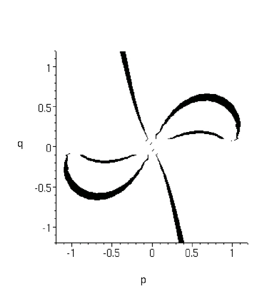
Figure 1: Intersection of three surfaces in $\alpha=0.5$

4.3 General Solutions

The big open question concerning spiral galaxies is whether dark matter exists or not and, amongst the class of spiral galaxies, it is the Low Surface Brightness (LSB) galaxies which present the most extreme problems. Typically, these objects are estimated to consist of more than $99\%$ dark matter, according to the canonical viewpoint. Therefore, it is these objects which must be successfully modelled by any new theory if that theory is to have maximum credibility.

Numerical techniques appear to offer the only realistic possibility for modelling specific galaxies. But, there are serious problems even here: specifically, the first galaxy in the LSB class was only discovered in the late 1980s and, even today, there are only a few tens of them with detailed and accurate rotation velocity measurements. Of these, only a minor fraction have detailed estimates of the ordinary matter in their discs and none have any radial flow measurements. In general, we would therefore expect that the detailed modelling of any specific LSB would necessarily require sweeping assumptions to be made about radial flows - thereby considerably reducing the value of any such modelling process (especially so when the equations concerned are numerically stiff).

However, in the case of the present theory, it transpires that the radial velocity component can be algebraically eliminated from the complete system, leaving a reduced system in rotation velocity and mass density only.

4.3.1 Mass Distribution: The Beautiful Equation

Not only is it possible to eliminate the radial velocity explicitly from the complete system, but the mass equation can be expressed in a form which is independent of velocity at all! In this form, it is given by:

$$(\psi^{2}-1)\epsilon^{2}+\frac{2}{q}\left[p(1+\psi^{2})+(1+p^{2}+q^{2})S\,\psi\right]\epsilon-(\psi^{2}-1)=0\,,$$ (4)

$${\rm where}~{}~{}~{}\epsilon^{2}\equiv-1-\frac{R}{\rho}\,\frac{d\rho}{dR}~{}~{}~{}{\rm and}~{}~{}~{}\psi^{2}\equiv 1-\frac{2\pi\rho}{m_{0}}\,R^{2}.$$ (5)

Here, $S=\pm 1$ whilst the parameters $(p,q,m_{0})$ are integration constants. Of these $(p,q)$ are as in §4.1, whilst $m_{0}$ can be fixed to have a magnitude of $4M_{gal}$ where $M_{gal}$ is the mass of the object being modelled estimated from measurements of stars, gas and dust. Since this is fixed independently of any calculations then there are, in effect, only two disposable parameters, $(p,q)$, for the mass and circular velocity equations. It is the algebraic structure of the mass equation above which, ultimately, allows the theory to model the various complexities manifested by rotation curves as a class, and which leads us to refer to it as the beautiful equation.

At face value - and when the signature $S=\pm 1$ is taken into account - equation (4) is satisfied by any one of four distinct distributions for $\rho$. However, the situation is more complex than this: reference to (4) shows that if $\epsilon=\pm 1$, then $\psi$ assumes one of two possible constant values. It then follows, by the second of (5), that $\rho\sim 1/R^{2}$. But any $\rho$ of this form also satisfies the first of (5). The net result is that the mass equation, (4), is satisfied when $\rho$ satisfies any one of six possible distributions.

However, closer analysis then reveals that of the two possibilities associated with $\epsilon=\pm 1$, one is not physical (it corresponds to negative densities) and of the four possibilities associated with $\epsilon\neq\pm 1$, a further one is also not physical. The net effect is that (4) is satisfied by any one of four physically realizable distributions for $\rho$ - so that, in principle, the distribution of material in any given galaxy disc can satisfy different differential equations over different anular sections. For example, the single admissable $\rho$ distribution corresponding to $\epsilon=\pm 1$ actually corresponds to the solution of §4.1, and we find that six of our sample of eight LSBs have such segments embedded within their discs.

4.3.2 The Rotation Velocity Distribution

The rotation velocity equation is given by given by

$$\frac{1}{V}\frac{dV}{dR}=\frac{1}{R}\left[\frac{1}{2}(1+\epsilon^{2})-\frac{p}{q}\,\epsilon-\left(\frac{p^{2}+q^{2}}{q}\right)\,\frac{\epsilon}{S\,\psi}\right]$$ (6)

where we note that $\rho$ appears through $\epsilon$ and $\psi$.

In practice, we have found that one (or two) switches between different $\rho$ distribution laws - and hence between different velocity distribution laws - occur somewhere in every LSB disc, and it is this mechanism which allows the theory to model the complex behaviour of rotation curves. We show the results of a detailed modelling exercise on a sample of eight LSBs in §7.

4.3.3 General Comments

It is interesting to note that, if $V=V^{*}$ is a solution of (6), then so is $V=kV^{*}$, for any constant $k$. This is a useful property in the present context since, because galaxy discs are generally not seen edge on, we can only estimate rotation velocities when we have estimated disc-inclination - and the effect of getting this wrong is simply to scale the true rotation velocities by an unknown constant factor. Thus, (6) is indifferent to knowledge about disc-inclination angles.

Finally, we note that the existence of a switching mechanism in the theory is reminiscent of the similar thing which is a necessary component of the MOND algorithm, discussed in later sections.

5 Power Law Dynamics: The Observations

5.1 General Comments

In this section, we give a brief review of the published evidence supporting the view that velocity distributions in idealized logarithmic discs behave according to the basic power law solutions, (1). There are four preliminary comments:

• Firstly, it is essential to understand that, so far as the phenomenology is concerned, we are only talking about rotation curves over their interior segments on which they are rising strongly - that is, we are explicity excluding the exterior flat parts. As it happens, practical considerations ensure that optical rotation curves are generally confined to this region anyway, and the analyses which follow are all confined to optical rotation curves (ORCs).

• Secondly, whilst a large amount of $V_{\theta}$ (circular velocity) data exists in the form of several large samples of published ORCs, there is no corresponding body of data for radial velocity flows. The reason is simply that such flows are, typically, an order of magnitude smaller than the circular flows and the techniques to measure them have only recently become available.

• Thirdly, our analysis applies only to idealized discs defined to possess perfect cylindrical symmetry. Since spiral galaxies typically possess bulgy central regions then our model can, at best, only have validity in those parts of the disc which are exterior to the innermost central regions and (by the initial comment) interior to the very outermost regions where the rotations curves become flat.

• Fourthly, since galactic discs are generally complete with all manner of irregularities then the model can only have a statistical validity. It is for this reason that we confine our selves to the analysis of very large samples only.

5.2 The ORC Samples

Mathewson, Ford & Buchhorn [1992] published a sample of 900 optical rotation curves (ORCs) which provided the basis for our first large scale analysis of disc dynamics from a power-law point of view. The results of this analysis, (Roscoe [1999a]) showed that the power-law resolves disc dynamics in the outer part of optical discs to a very high degree of statistical precision. We have subsequently analysed three further large samples, these being those of the 1182 ORCs published by Mathewson & Ford [1996], the 497 ORCs published by Dale et al ([1997] et seq) and the 305 ORCs published by Courteau [1997]. This last sample differs from the previous three in being the only one using $R$-band photometry rather than $I$-band photometry. For associated technical reasons, the modelling process for the Courteau sample differs in its details from the others and so is excluded from the first part of the present discussion.

5.3 The Basic $(\alpha,\ln A)$ Plot

The basic question is: does the power-law $V_{rot}=AR^{\,\alpha}$ provide a good resolution of ORC data on the exterior part of optical discs ? (Remember, practical considerations ensure that ORCs generally to not extend to the far exterior regions where rotation curves become flat). The first problem here is to give an objective definition of what is meant by the exterior part of the optical disc. This is provided originally in Roscoe [1999a], and more clearly in Roscoe [$2002$b]. Once this is done, the analysis uses linear regression to estimate the parameter pair $(\ln A,\,\alpha)$ for each of the ORCs in the sample. Figure 2 gives the scatter plot for all of the 2405 usable ORCs in the three $I$-band samples. (About 7% of the total sample of 2579 ORCs were lost to the analysis because of objective reasons associated with data quality.)

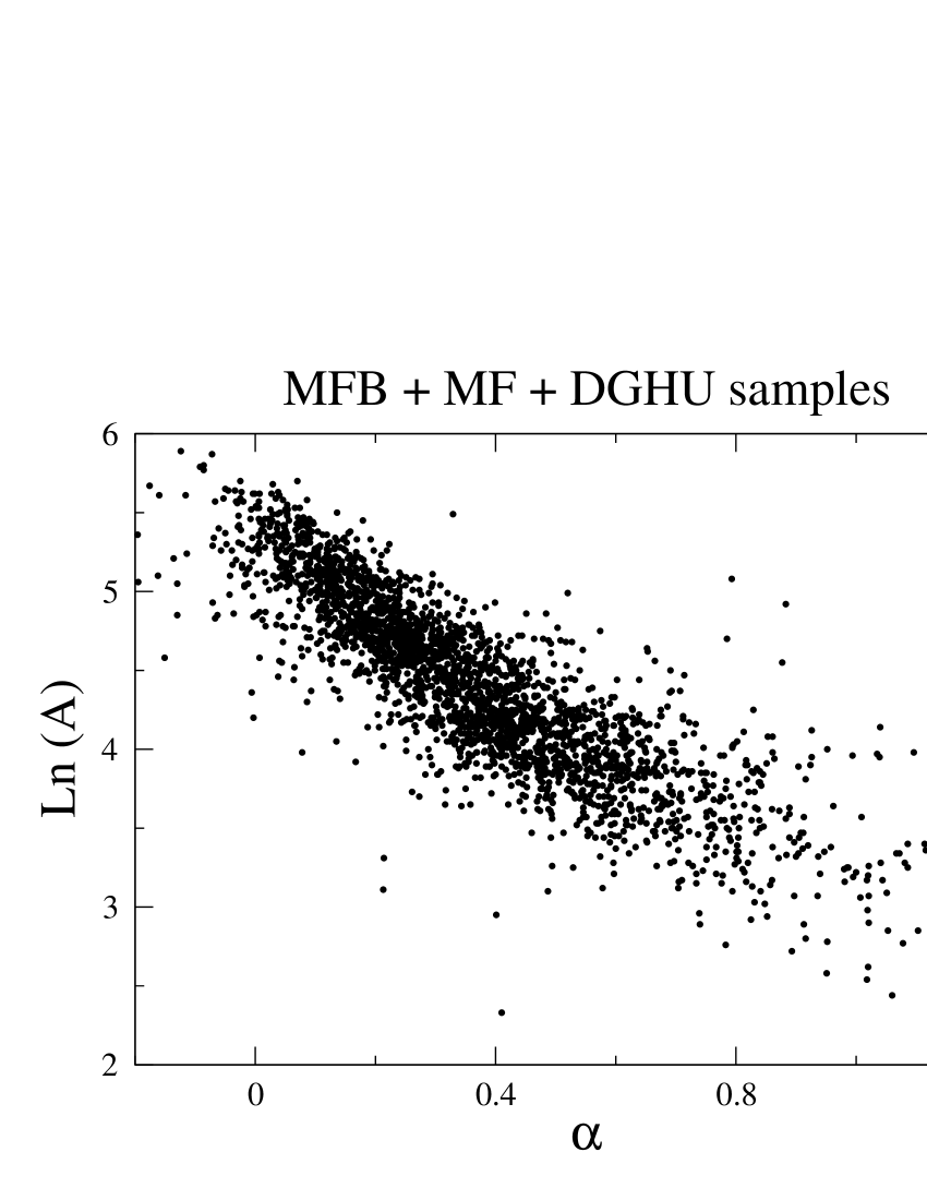
Figure 2: Plot of $(\ln A,\,\alpha)$ for 2405 galaxies

There are three significant points to be made:

• The first point, which came as a shock, is the existence of a very clear and powerful correlation between $\ln A$ and $\alpha$, since there is no obvious apriori reason why any correlation should exist at all;

• Secondly, although there is no apriori reason to expect an $(\alpha,\ln A)$ correlation, equation (2) states that $\alpha$ is correlated with the dynamical parameters $(p,q)$. But, by definition, $\ln A$ is strongly determined by the dynamics and so it follows that, in qualitative terms, the $(\alpha,\ln A)$ correlation of figure 2 is consistent with the existence of a relation like the $\alpha$-constraint of (2);

• Thirdly, except for what is probably statistical scatter, $\alpha$ appears to be strongly confined in the region $\alpha\in(0,1)$. In section §7.5, we see how this $\alpha$ confinement has an elegant association with certain topological transitions in the $(\alpha,p,q)$ parameter space.

5.4 A Detailed Model of the $(\alpha,\ln A)$ Plot

A more detailed analysis of this diagram showed that the luminosity properties of galaxies vary very strongly through the plot. Specifically, consider the power-law model, $V=A\,R^{\,\alpha}$, in dimensionless form:

$${V\over V_{0}}\,=\,\left({R\over R_{0}}\right)^{\alpha}~{}~{}\rightarrow~{}~{}A\,=\,{V_{0}\over R_{0}^{\,\alpha}}\,.$$ (7)

Then, defining $M$ as the absolute $I$-band magnitude and $S$ as the absolute $I$-band surface brightness of an object, a detailed modelling of the MFB (Mathewson et al [1992]) and MF (Mathewson & Ford [1996]) data in figure 2 shows that the particular model

$$\ln A = \ln V_{0}-\alpha\,\ln R_{0},$$

$$\ln V_{0} = -1.596-0.316\,M$$ (8)

$$\ln R_{0} = -7.614\,-0.474\,M-0.0050\,S$$

accounts for about 93% of the total variation in the figure. It is to be noted that, in the model, the $t$-statistic for each of the model parameters satisfies $|t|>11$, so that all the included variations are powerfully present. This is, in itself, a strong demonstration of how effectively the power-law model resolves ORC data. The model fit can be improved by including the DGHU (Dale et al [1997] et seq) data in the modelling process - but we choose to exclude it to provide an independent test, discussed below.

5.5 An Alternative Visualization of the Model-Fit

A very effective alternative way of visualizing the fit of the model (8) to the data can be obtained as follows: Suppose we use the definitions of (8) in the dimensionless form give at (7), so that the measured $(R,\,V)$ data for each ORC is scaled by the luminosity models for $(R_{0},\,V_{0})$ for that ORC, and then regress $\ln(V/V_{0})$ on $\ln(R/R_{0})$ for each ORC. Then, if the power-law model (7) is good, we should find a null zero point for each ORC - except for statistical scatter.

Figure 3 (left) gives the frequency diagram for the actual zero points computed for the combined Mathewson et al ([1992], [1996]) samples from which the model (8) was derived, whilst a wholly independent test of the model is given by figure 3 (right) which gives the frequency diagram for the zero points derived from the DGHU sample using the model (8) - which, of course, was derived without DGHU data. It is clear that there is absolutely no evidence to support the idea that these zero points are different from the null position. Thus, the power-law model is strongly supported, and (7) with (8) can be considered to give a high precision statistical resolution of ORC data in the exterior part of the disc.

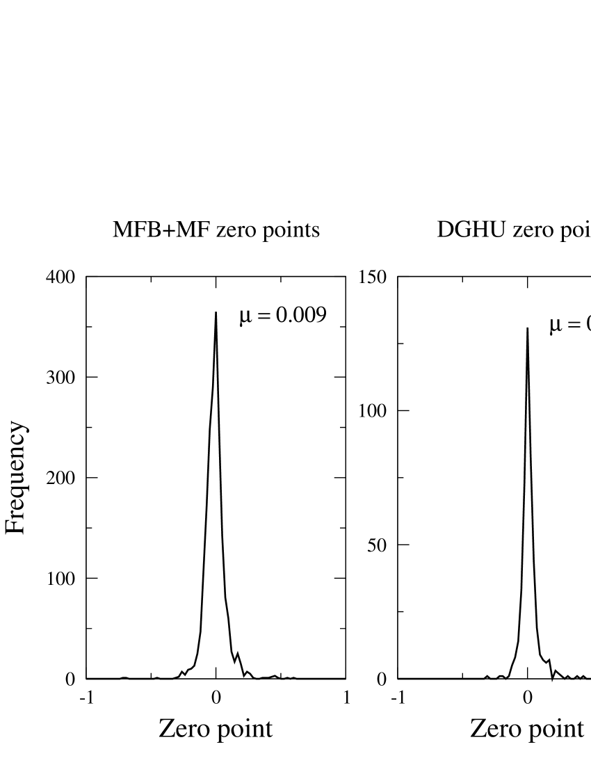
Figure 3: Plot of zero point for 1951 MFB+MF galaxies and 454 DGHU galaxies

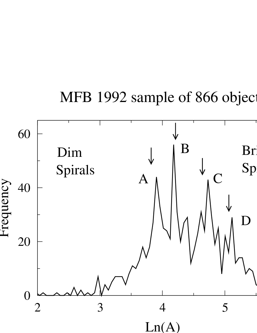
Figure 4: Vertical arrows represent predicted positions of peaks from an analysis of 12 Rubin et al ORCs

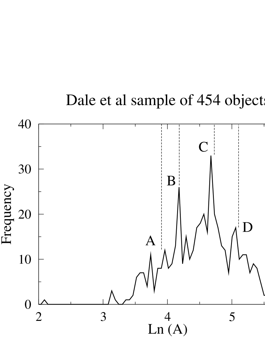
Figure 5: Vertical dotted lines indicate peak centres of figure 4.

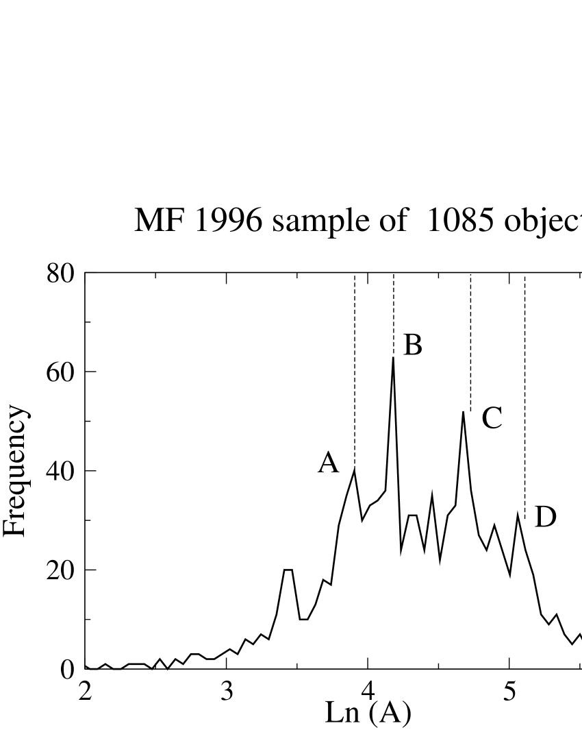
Figure 6: Vertical dotted lines indicate peak centres of figure 4.

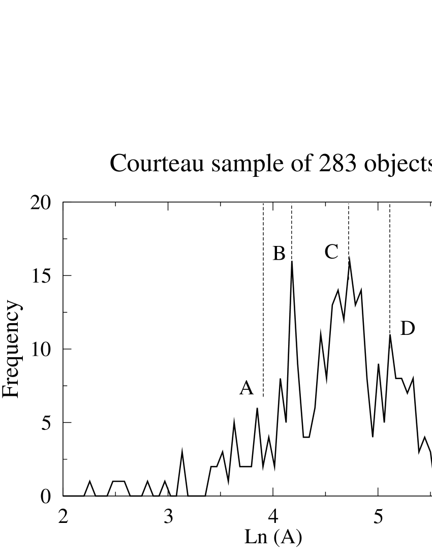
Figure 7: Vertical dotted lines indicate peak centres of figure 4.

To summarize, we have so far shown that the rotational part of the power-law model (1) is very strongly supported on the data and have indicated that the data does not yet exist to consider the validity - or otherwise - of the radial component of the model.

6 Discrete Dynamical Classes: The Observations

6.1 General Comments

In this section we consider the exact solutions of §4.1 - specifically, we consider the extremely strong statement, made at (3), to the effect that $\alpha$, calculated for any given spiral, is constrained to occupy one of a set of distinct surfaces in $(\alpha,\,p,\,q)$ space, where $(p,\,q)$ are dynamical parameters in the model.

This statement has interest on many levels - not least because nothing like it features in any other extant theory of disc dynamics. The effect was first noticed - tentatively and prior to us recognizing the potential significance of the $\alpha$-constraints - during a pilot study of a small sample of Rubin et al [1980] ORCs, and this initial identification was used to define a hypothesis which was subsequently tested on the Mathewson et al [1992] sample, and reported in Roscoe [1999b]. The effect was subsequently confirmed in Roscoe [$2002$b] on three further large samples (Dale et al [1997] et seq, Mathewson & Ford [1996] and Courteau [1997]). For completeness, we give a brief review of this evidence here.

In practice, the evidence takes the form of the $\ln A$ frequency diagrams for each of the four samples, and then interpreting the meaning of these diagrams. The computation of the $\ln A$ parameter is as it was for figure 2 (but see Roscoe [$2002$b] for a complete discussion).

6.2 The $\ln A$ Frequency Diagrams

Figure 4 shows the $\ln A$ distribution arising from the analysis of the Mathewson et al [1992] sample, and the short vertical arrows in that figure indicate the predicted positions of the peaks, based on a pilot study of a sample of twelve ORCs from Rubin et al [1980]. Given the very small size of this initial sample of Rubin objects, we can see that the match is remarkable.

Figures 5, 6 and 7 show the corresponding distributions for the Dale et al ([1997] et seq) sample, the Mathewson & Ford [1996] sample and the Courteau [1997] sample. In each of these cases, the vertical dotted lines indicate the peak centres of figure 4.

The $A$ peak in figures 5 and 7 are more-or-less absent because this peak corresponds to very dim objects, and these are very much under-represented in the two samples concerned.

The joint probability of the observed peaks in the four samples arising by chance alone, given the original hypothesis raised on the small Rubin et al sample, has been computed in Roscoe [$2002$b], using extensive Monte-Carlo simulations, to be vanishingly small at $\approx 10^{-20}$.

6.3 Interpretation of the $\ln A$ Frequency Diagrams

It is clear from the four diagrams that $\ln A$ has a marked preference for one of four distinct values, say $\ln A\,=\,k_{1},\,k_{2},\,k_{3},\,k_{4}$. However, we also know, from §5.4, that $\ln A$ is a strongly defined function of the galaxy parameters $(\alpha,\,M,\,S)$, so that $\ln A=F(\alpha,\,M,\,S)$. Putting these two results together gives

$$F(\alpha,\,M,\,S)\,=\,k_{i}\,,~{}~{}~{}~{}i=1,2,3,4\,.$$ (9)

Consequently, the $\ln A$ frequency diagrams imply that spiral discs are confined to one of four distinct surfaces in $(\alpha,\,M,\,S)$ space.

But $M$ is a measure of absolute galaxy luminosity, and therefore a measure of the corresponding total galaxy mass, $m$ say (assuming no dark matter). Similarly, the surface brightness parameter, $S$, which is a measure of the density of absolute galaxy luminosity, can be considered as a measure of mass density, $\rho$, in a galaxy. That is, $(M,\,S)\approx(m,\,\rho)$ and these latter two parameters are, apriori, important dynamical parameters for any given system. If we now presuppose the existence of a mapping $(m,\rho)\rightarrow(p,q)$ where $(p,q)$ are the dynamical parameters in our model equations, then we see that (9) is consistent with (3) - the difference being that (3) allows up to six surfaces, whereas we have only identified four in the phenomenology.

We reasonably state, therefore, that the theory contains all the structure required to explain, in principle, the phenomenon of discrete dynamical classes for disc galaxies - subject to the existence of appropriate mappings $(m,\rho)\rightarrow(p,q)$. However, various significant details uncovered in the analysis of §7 give us further insight into the problem, and these are briefly discussed in §8.

7 Detailed Modelling of LSB Galaxies

In this section, we apply equations (4) and (6) of §4.3 to the detailed modelling of a sample of eight LSB galaxies which have already been successfully modelled by MOND (deBlok & McGaugh [1998] and McGaugh & deBlok [1998b]). We shall not dwell on the computational problems involved in solving these equations, but we shall discuss, briefly, the means by which the parameters $(m_{0},p,q)$ were determined.

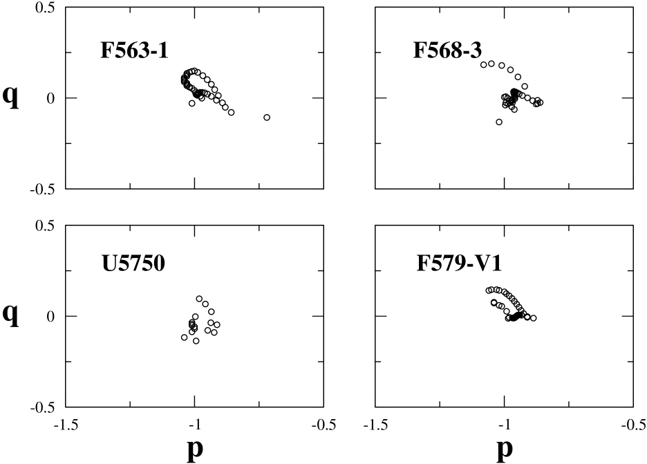
Figure 8: Numerical estimates of $(p,q)$. Note: Each box is a unit box in the $(p,q)$ plane.

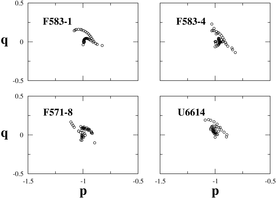
Figure 9: Numerical estimates of $(p,q)$. Note: Each box is a unit box in the $(p,q)$ plane.

7.1 The Parameter $m_{0}$

Referring to (4), and noting that $\rho$ in this equation is the density of material in a disc of unit thickness, we can deduce from the definition of $\psi$ given there that $m_{0}$ has dimensions of mass. This suggests that it is likely to be a simply related to the total mass of the object being modelled. In fact, we found that, defining $M_{gal}$ as the total or ordinary mass (stars + dust + gas) in the galaxy being modelled (as estimated by the original observing astronomer - Stacy McGaugh in the present case), then $m_{0}=4M_{gal}$ worked extremely well for all eight cases.

7.2 Estimating The Parameters $(m_{0},p,q)$

We comment firstly that the theory is indifferent to the signatures of $p$ and $q$ but, for the sake of being explicit, we take them to be always negative. With this proviso, then as a means of (a) obtaining estimates of $(m_{0},p,q)$ for each LSB in the sample and (b) providing a preliminary consistency check on the model equations (4) and (6), we proceeded as follows:

• Assume that $m_{0}$ is some simple multiple (fixed for all the objects) of estimated total mass (obtained by integrating McGaugh’s data for each object);

• For each LSB, use the McGaugh mass-distribution estimates and rotation velocity measurements to obtain smooth cubic spline models of mass and velocity distributions;

• Use these smooth cubic spline models to obtain estimates of density, density gradient, velocity and velocity gradient at a sequence of distinct points across the disc of each LSB;

• With these estimates, the differential equations , (4) and (6), at any given point in a disc become two algebraic equations for determining $(p,q)$;

• For each LSB, solve this pair of algebraic equations at several points across the disc, and look for consistency in the resulting sequence of estimates of $(p,q)$.

A necessary condition of the theory’s consistency is that, for some reasonable choice of $m_{0}$, the foregoing process will lead to a consistent set of $(p,q)$ estimates across each LSB disc.

In fact, we found that setting $m_{0}=4M_{gal}$, where $M_{gal}$ is the estimated total of ordinary galaxy mass (stars+dust+gas) for each LSB, gave a very consistent picture for estimates of $(p,q)$. The big surprise was that, not only was this the case for each individual object, but that the set of $(p,q)$ pairs for the whole sample lies in the same very small neighbourhood of the $(p,q)$ plane. Figures 8 and 9 show the results of this latter exercise for each of the eight LSBs in our sample, and we see that, for each object, the $(p,q)$ estimates all lie in the neighbourhood of $(-1,0)$ in the $(p,q)$ plane. Note: for each LSB, solutions were sought in a very large $(20\times 20)$ region of the $(p,q)$ plane. The only solutions found are those indicated.

This exercise allowed us to conclude that the model equations were highly consistent with the phenomenology, and also gave us a good starting estimate of $(p,q)\approx(-1,0)$ for the detailed modelling process of each object in the sample.

Table 1:

Galaxy	$p$	$q$
F563-1	-0.990	-0.038
F568-3	-0.970	-0.004
U5750	-0.955	-0.158
F579-V1	-0.997	-0.022
F583-1	-0.980	-0.047
F583-4	-0.950	-0.084
F571-8	-0.952	-0.041
U6614	-0.995	-0.032

7.3 The Detailed Models

The integrated solutions for the rotational velocities and the mass distributions (using the $(p,q)$ estimates listed in Table 1), together with the corresponding observational measurements, are given in Figures 10 & 11. In every case, we see that the fit of the computed rotation velocities (solid lines) to the measured rotation velocities (filled circles) is, for all practical purposes, perfect.

Except for discrepencies near galactic centres, where our modelling assumptions become less good, our computed density distributions (dotted lines) provide reasonable fits to the estimated densities (crosses). However, it is important to realize that, by contrast with the accuracy of Doppler velocity measurements, mass estimation in galaxy discs is subject to very great uncertainties - which is why mass-modellers never quote error-bars for their estimates. We have used McGaugh’s mass-models to estimate our parameter $m_{0}$, mentioned earlier. But, for the mass-density integration, we have chosen the initial conditions to ensure that the predicted mass distributions over the discs provide good qualitative fits to MacGaugh’s models.

Finally, it should be remarked that all dark matter models fail comprehensively when applied to LSBs - MOND (described in detail in §11) has been successfully applied to all of the objects considered here (deBlok & McGaugh [1998] and McGaugh & deBlok [1998b]) and to a great many more.

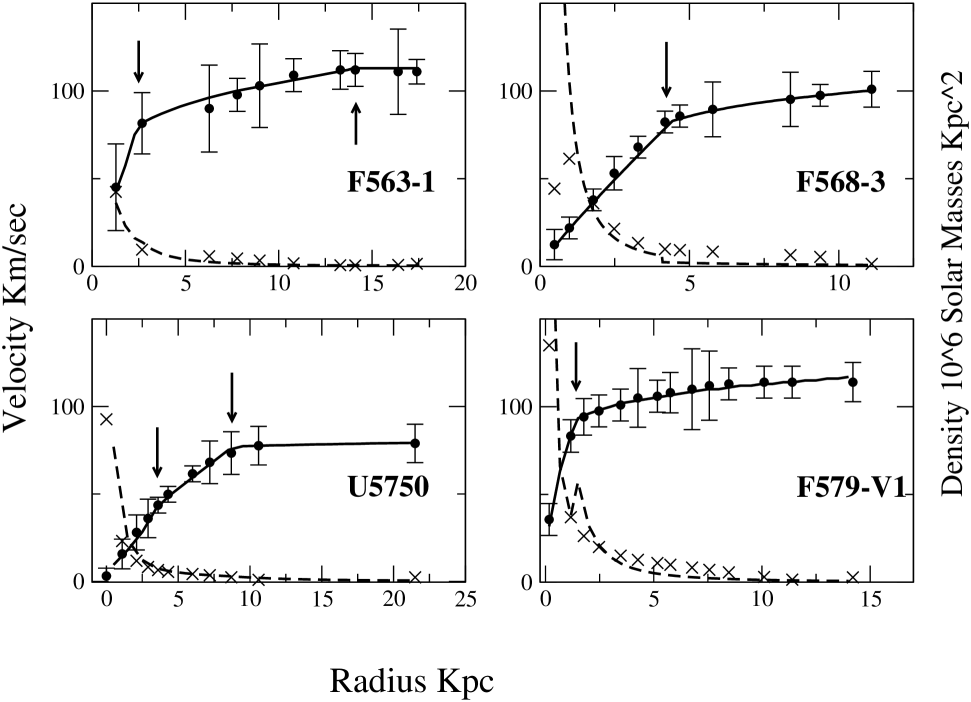
Figure 10: Solid line = calculated velocity; dotted line = calculated mass density; circles = measured velocities with error bars; crosses = estimated mass density. Arrows = switch-points.

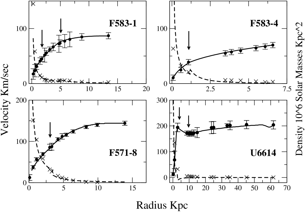
Figure 11: Solid line = calculated velocity; dotted line = calculated mass density; circles = measured velocities with error bars; crosses = estimated mass density. Arrows = switch-points.

7.4 Remarkable Circumstantial Evidence

We have already noted how, for each LSB in the sample, $(p,q)\approx(-1,0)$. This circumstance allows us to discover a remarkable connection between the phenomenology, as represented by these particular $(p,q)$ values and the theory as represented by the surfaces $\alpha=F_{i}(p,q),~{}i=1..6$ defined at (2).

Specifically, we know that, in practice, it is virtually always the case that $0<\alpha<1$ (see Figure 2, for example) so that we might expect the intersection of these surfaces with the plane-surface $\alpha=0.5$ to give a fairly typical cross-section. Figure 12 shows this cross-section in the neighbourhood of $(p,q)=(-1,0)$, which contains our LSB sample. We see immediately that the point $(p,q)=(-1,0)$ enjoys a very special status in this $\alpha=0.5$ plane - it is, in fact, the point of intersection of four distinct surfaces from the set $\alpha=F_{i}(p,q),\,i=1..6$ with the plane $\alpha=0.5$. Closer investigation reveals that $(p,q)=(-1,0)$ retains its status as a special nodal point for all $(0<\alpha<1)$, and is therefore a distinguished axis for the theory.

So, we have the circumstance that our LSB sample lies in the neighbourhood of a distinguished axis of the theory defined by the intersection of four particular surfaces. Whilst it is probably not possible to say what the meaning of this is at present (we need larger samples of LSBs and corresponding samples of ordinary spirals with complete mass models), there is a very good chance that it represents a circumstance of considerable significance in the overall context of galactic evolution and dynamics.

Figure 12: Intersection of $\alpha=F_{i}(p,q),~{}i=1..6$ in the plane $\alpha=0.5$

Figure 13: Intersection of $\alpha=F_{i}(p,q),~{}i=1..3$ in the planes $\alpha=1.5,0.5,0.0,-0.5$

7.5 Global Complex Structure and $\alpha$ Phenomenology

Figure 13 shows the evolution of three of the six surfaces as $\alpha$ varies in the range $(1.5,-0.5)$ (the three omitted surfaces are mirror images of the three shown). At $\alpha=1$ (not explicitly shown) there is a degeneracy as the three curves merge identically along the $q=0$ axis whilst, at $\alpha=0$ (explicitly shown), there is a degeneracy in which two of the curves merge identically, although not along any axis. Thus, the two values $\alpha=0$ and $\alpha=1$ which, according to figure 2, appear to bound the phenomenology, are also each associated with degenerate transitions of the surface topology.

8 More On The Discrete Dynamical Classes Phenomenology

The LSB modelling exercise of §7 was significant at two levels:

• firstly, it showed how the theory successfully models the details of LSB dynamics and mass distributions;

• secondly, it led us to the significant discovery that LSBs are strongly associated with the distinguished axis $(p,q)=(-1,0)$ in the $(\alpha,p,q)$ parameter space.

The second point poses questions relevant to gaining a detailed understanding of the discrete dynamical states phenomenology. Specifically, according to the discrete dynamical states phenomenology, low-luminosity spirals are associated with the $A$-state typified in figure 4. The LSBs of our sample are, by definition, low-luminosity spirals and are therefore, presumably, $A$-state spirals. But, we have also seen that these LSBs are strongly associated with the distinguished axis, $(p,q)=(-1,0)$, and so the obvious question now is: what is the distribution of higher-luminosity spirals ( that is, $B$, $C$ and $D$-state spirals) in the $(p,q)$ plane?

This question must be answered before we can begin to understand the discrete dynamical states phenomenology in any detailed way. But, at the moment, we cannot address this question rigorously, simply because we do not have available a sample of higher-luminosity spirals with detailed estimated mass distributions (stars+dust+gas). The reason for this lack of data is simple: since, according to the canonical view, $>95\%$ of galaxy mass is CDM then there is no point in constructing detailed maps of the distribution of ordinary matter in galaxy discs. This exercise has only been done systematically (and for LSBs only) by astronomers interested in the MOND vs CDM debate.

However, there is a possible way forward: for every one of the $\approx 2500$ ordinary spirals used in the four discrete dynamical states analyses we have $I$-band (or $R$-band) photometry. In principle, such photometry can be used to derive broad-brush estimates of ordinary mass distributions which, combined with large statistics, might be sufficient for the task at hand. This is for future work.

9 The Detailed Dynamical Theory

In the following, we finally detail the application of the basic theory to the modelling of an idealized spiral galaxies - defined to be one without a central bulge, and without the irregularities that are routinely present in the discs of real galaxies, and without the bars that are present in many spirals. We model this idealized spiral galaxy as a mass distribution possessing perfect cylindrical symmetry.

We know, from the considerations of §F.1, that the general form of the metric tensor, for any given material distribution, is

$$g_{ab}\equiv\nabla_{a}\nabla_{b}U\equiv{\partial^{2}{\cal M}\over\partial x^{a}\partial x^{b}}-\Gamma^{k}_{ab}{\partial{\cal M}\over\partial x^{k}},$$

where $\Gamma^{k}_{ab}$ represents the metrical affinity and where, by the conjecture of §3.2, the value of ${\cal M}({\bf r})$ is to be generally understood as a measure of the amount of (ordinary) mass contained within the level surface passing through the point with position vector ${\bf r}$ defined with respect to the mass-centre of the ordinary perturbing matter distribution. In the present case, of course, the level surfaces are infinite cylinders, and so we have to modify the definition so that ${\cal M}({\bf r})$ refers to the mass contained within cylinders of unit thickness. With this understanding, and remembering that ${\cal M}^{\prime}\equiv d{\cal M}/d\Phi$ and that $\Phi=R^{2}/2$, it is easily shown that ${\cal M}^{\prime}\equiv 2\pi\rho$, where $\rho$ is the mass density in a disc of unit thickness.

Noting that the geometry on any level-surface of a cylindrical distribution is Euclidean, it follows that the $\Gamma^{k}_{ab}$ are identically zero in the present case. Consequently,

$$g_{ab}={\partial^{2}{\cal M}\over\partial x^{a}\partial x^{b}}\equiv{\cal M}^{\prime}\delta_{ab}+{\cal M}^{\prime\prime}x^{a}x^{b},$$ (10)

where we remember ${\cal M}^{\prime}\equiv d{\cal M}/d\Phi$ and $\Phi\equiv R^{2}/2$ (this latter notation simplies the algebra). Defining the Lagrangian density

$${\cal L}\equiv\sqrt{g_{ij}{\dot{x}}^{i}{\dot{x}}^{j}}=\left({\cal M}^{\prime}<{\dot{\bf R}}|{\dot{\bf R}}>+{\cal M}^{\prime\prime}{\dot{\Phi}}^{2}\right)^{1/2},$$

where ${\dot{x}^{i}}\equiv dx^{i}/dt$ etc., the equations of motion are found from the Euler-Lagrange equations as

$$2{\cal M}^{\prime}{\bf{\ddot{R}}}+\left(2{\cal M}^{\prime\prime}{\dot{\Phi}}-2{{\dot{\cal L}}\over{\cal L}}{\cal M}^{\prime}\right){\bf{\dot{R}}}$$ (11)

$$+\left({\cal M}^{\prime\prime\prime}{\dot{\Phi}}^{2}+2{\cal M}^{\prime\prime}{\ddot{\Phi}}-{\cal M}^{\prime\prime}<{\bf{\dot{R}}}|{\bf{\dot{R}}}>-2{{\dot{\cal L}}\over{\cal L}}{\cal M}^{\prime\prime}{\dot{\Phi}}\right){\bf R}=0.$$

However, it is obvious that the Lagrangian density, defined above, will lead to a variational principle which is degree zero in the ‘time’ parameter. It follows that the equations of Euler-Lagrange pair, above, cannot be linearly independent. Whilst either equation can therefore be chosen, it transpires that the ${\bf\hat{\theta}}$ component equation is algebraically less complicated.

9.1 The ${\bf\hat{\theta}}$ component

We have

$$2{\cal M}^{\prime}(R\,{\ddot{\theta}}+2\,{\dot{R}}\,{\dot{\theta}})+R{\dot{\theta}}\left(2{\cal M}^{\prime\prime}{\dot{\Phi}}-2{{\dot{\cal L}}\over{\cal L}}{\cal M}^{\prime}\right)=0.$$

Multiply through by $R/2{\cal L}$ and use ${\cal M}^{\prime\prime}{\dot{\Phi}}\equiv{\dot{\cal M}^{\prime}}$ to get, after some rearrangement:

$$\left({{\cal M}^{\prime}\over{\cal L}}\right)\,{d\over dt}(R^{2}{\dot{\theta}})+R^{2}\,{\dot{\theta}}\,\left({{\cal L}\,{\dot{\cal M}^{\prime}}\,-\,{\dot{\cal L}}\,{\cal M}^{\prime}\over{\cal L}^{2}}\right)=0\,.$$

This integrates directly to give:

$${d\over dt}\,\left\{R^{2}\,{\dot{\theta}}\,\right.\left.\left({{\cal M}^{\prime}\over{\cal L}}\right)\right\}=0,$$

from which we see that angular momentum is not generally conserved. Consequently, the net disc forces are not, in general, central forces so that, correspondingly, there exists a mechanism for transferring angular momentum through the disc. This latter equation integrates to give:

$$({\cal M}^{\prime})^{2}\,R^{2}\,V_{\theta}^{2}=m_{0}\left[({\cal M}^{\prime}+{\cal M}^{\prime\prime}\,R^{2})\,V_{R}^{2}+{\cal M}^{\prime}\,V_{\theta}^{2}\right]$$ (12)

where $V_{R}\equiv{\dot{R}}$ and $V_{\theta}\equiv R\,{\dot{\theta}}$.

9.2 Completion of the Dynamical System

The cylindrical symmetry of the idealized spiral galaxy implies that there is net zero force out of the plane of the galaxy. It follows that the ‘self-similar’ dynamics condition (cf §F.2), which must be used in conjunction with (12), to close the system can be written as:

$${Transverse~{}Accn\over Radial~{}Accn}=k_{0}.$$ (13)

where, because of the radial symmetry of the system, $k_{0}$ has the same value along all radial directions. To obtain the quantitative form of this, we need expressions for the radial and transverse accelerations in the disc geometry. These are derived in appendix H, and we find that (13) becomes

$$- k_{0}\,S\,\sqrt{{{\cal M}^{\prime}+{\cal M}^{\prime\prime}\,R^{2}\over{\cal M}^{\prime}}}\,V_{R}\,{dV_{R}\over dR}\,+\,V_{R}\,{dV_{\theta}\over dR}=$$ (14)

$$- \left(S\,\sqrt{{\cal M}^{\prime}+{\cal M}^{\prime\prime}\,R^{2}\over{\cal M}^{\prime}}\,+\,{{\cal M}^{\prime\prime}\over 2\,{\cal M}^{\prime}}\,R^{2}\,\right)\,{{V_{R}}\,{V_{\theta}}\over R}$$

$$+ \,k_{0}\,{\left(S\,{3{\cal M}^{\prime\prime}+{\cal M}^{\prime\prime\prime}\,R^{2}\over 2\,\sqrt{{\cal M}^{\prime}({\cal M}^{\prime}+{\cal M}^{\prime\prime}\,R^{2})}}\,R\,{V_{R}}^{2}\,-\,\,{V_{\theta}^{2}\over R}\right)}\,$$

where $S=\pm 1$.

Remembering that ${\cal M}^{\prime}=2\pi\rho$ (cf start of §9), we now note that the expression ${\cal M}^{\prime}+{\cal M}^{\prime\prime}{R}^{2}$ is negative if $\rho$ drops off more quickly than $1/R$ - which, in practice, always seems to be the case. The implication of this practical reality is that $k_{0}$ is actually complex so that the two equations (12) and (14) represent three equations in the three unknowns $(V_{\theta},V_{R},{\cal M}^{\prime})$, and not just two. It is when $V_{R}$ is eliminated between these three equations that we obtain equations (4) and (6) of §4.3.

However, we initially overlooked the possibility that ${\cal M}^{\prime}+{\cal M}^{\prime\prime}{R}^{2}$ might be negative and, consequently, believed we needed a further equation to close the system completely. As it happens, our approach to obtaining this extra equation gave ${\cal M}^{\prime}+{\cal M}^{\prime\prime}{R}^{2}<0$ anyway, and effectively picked out a special solution of the above system, and is described in the following section.

10 A Special Case Solution: The Logarithmic Disc

Our oversight led us to believe that a further equation was required to close the system. We argued as follows: It has been recognized for a very long time that, if the obvious irregularities which exist in spiral discs are ignored, then the spiral structure of spiral galaxies is essentially logarithmic. In the context of a classical disc, the most direct, way to interpret this phenomenology is to write

$${V_{\theta}\over V_{R}}\,=\,K_{1}$$ (15)

since this implies directly that disc streamlines are logarithmic spirals. Substitution of this into (12), and using ${\cal M}^{\prime}\equiv 2\pi\rho$, gives immediately

$${\cal M}^{\prime}\equiv 2\pi\rho={k_{2}\over R^{2}}$$ (16)

for some constant $k_{2}$. That is, the density of matter in the logarithmic disc behaves as an inverse square law. We quickly find that this implies ${\cal M}^{\prime}+{\cal M}^{\prime\prime}R^{2}<0$, so that we are back to the point we overlooked initially - that (14) represents, in fact, two distinct equations which must both be satisfied. More particularly, putting (15) and (16) into (14) we find

$$(K_{1}-k_{0}Sj)\frac{1}{V_{R}}\frac{dV_{R}}{dR}=-\frac{1}{R}((Sj-1)K_{1}+k_{0}(Sj+K_{1}^{2})),$$

where $S=\pm 1$ and $j=\sqrt{-1}$. Since solutions must be real, we must have $k_{0}$ complex. Putting $k_{0}=q+pj$, where $(p,q)$ are real parameters, then gives the two equations

$$\frac{1}{V_{R}}\frac{dV_{R}}{dR}=\frac{1}{R}\left(\frac{K_{1}-qK_{1}^{2}+pS}{pS+K_{1}}\right),~{}~{}~{}\frac{1}{V_{R}}\frac{dV_{R}}{dR}=\frac{1}{R}\left(\frac{SK_{1}+pK_{1}^{2}+qS}{qS}\right)\equiv\frac{\alpha}{R}$$ (17)

which must be identical. This latter requirement quickly gives that the parameters $(K_{1},p,q)$ must satisfy

$$pK_{1}^{2}+S(1+p^{2}+q^{2})K_{1}+p=0.$$ (18)

If we use this to eliminate the explicit appearance of $K_{1}^{2}$ in the second of (17), we get

$$\alpha=1-\frac{p}{Sq}-\frac{p^{2}+q^{2}}{q}K_{1}=1-\frac{p}{Sq}-\frac{p^{2}+q^{2}}{qK_{1}}.$$

The second expression for $\alpha$, which is the form given at (2), occurs since, if $K_{1}$ is a solution of (18), then so is $1/K_{1}$.

11 The MOND Programme

11.1 Overview of MOND

Modified Newtonian Dynamics (MOND) is an empirically motivated modification of Newtonian gravitational mechanics which can be interpreted as either a modification of Newton’s gravitational law, or as a modification of the second law (the law of inertia). See Milgrom [1994] for a comprehensive review. The basic idea was conceived by Milgrom [1983a], [1983b], [1983c], as a way of understanding the flat rotation curve phenomenology of spiral galaxies without recourse to the dark matter idea. The basic hypothesis is that, in extremely weak gravitational fields ($g<<10^{-10}ms^{-2}$), the nature of Newtonian gravitation changes in such a way that flat rotation curves are the natural result.

The quantitative idea can be briefly described as follows: if we use $g_{N}({\bf R})$ to denote the gravitational acceleration at any position ${\bf R}$ in a material distibution according to Newtonian theory, then the MOND prescription says that the actual gravitational acceleration is given by $g=\sqrt{a_{0}\,g_{N}({\bf R})}$ when the field is extremely weak. Here $a_{0}$ is a parameter which has been fixed (Begeman et al [1991]) for all applications of MOND to the value $a_{0}\,=\,1.2\times 10^{-10}\,ms^{-2}$. Thus, for a particle in a circular orbit about a point source of mass $M$, the acceleration-balance equation in the MOND limit of the very weak field would be given by

$${V_{rot}^{2}\over R}=\sqrt{{\gamma M\over R^{2}}\,a_{0}}~{}~{}\rightarrow~{}~{}V_{rot}=(\gamma\,M\,a_{0})^{1/4}\,,$$

where $V_{rot}$ is the circular velocity.

This simple idea, which in practice, leads to a model with only one free parameter (the so-called mass-to-light ratio, $\gamma^{*}\,\equiv\,M/L$, which gives the conversion factor from the observed light to the inferred mass), has been remarkably successful in explaining the phenomenology associated with a very wide variety of circumstances (de Blok & McGaugh [1998]). Furthermore, MOND makes several strong predictions (Milgrom [1983b]) and is therefore eminently falsifiable. It is notable, therefore, that it never has been although several attempts have been made (de Blok & Mcgaugh [1998]). This circumstance is to be compared with that of the conventionally favoured CDM (Cold Dark Matter) model. This latter model is a multi-parameter model, which makes no predictions - other than that of the existence of CDM - and can therefore never be falsified in the classical sense.

11.2 General Comments on MOND and the Present Theory

If the MOND prescription is an accurate reflection of the reality, then there necessarily exists an underlying theory of gravitation which provides flat rotation curves in the weak field regime independently of dark matter distributions. Conversely, any such theory - should it exist - must necessarily give rise to the basic MOND prescription, $g\,=\,\sqrt{a_{0}\,g_{N}({\bf R})}$, in the weak field when interpreted from a Newtonian perspective.

In the present case, flat rotation curves correspond to the degenerate $\alpha=0$ case discussed in §7.5. Thus, flat rotation curves solutions do exist in the presented theory, and are associated with a degeneracy, and are therefore special in some - yet to be understood - way. The inclusion of the qualitative aspects of MOND in the theory is already guaranteed by the simple fact that flat rotation curve solutions are admitted.

11.3 LSBs - Extreme Objects in MOND and the Present Theory

According to any given theory, when the mass/dynamical relations in a given spiral object cross a certain threshold specific to that theory, the object ceases to be gravitationally bound. In the early 1980s Milgrom realized that, according to MOND, there should exist spiral objects which were so diffuse that they could not possibly exist according to the canonical theory. These objects, now known as Low Surface Brightness galaxies (LSBs), were subsequently observed in the late 1980s. Of all astrophysical objects, these present the most critical conditions for the CDM models since, according to these models, LSBs must typically consist of more than 99% dark matter. Even so, it is now well recognized that the CDM models have suffered comprehensive failure when applied to model LSBs.

Beyond the initial prediction, the importance of LSBs to MOND can be summarized as follows: a common criticism of MOND is that, since it was designed to yield flat rotation curves in the very weak-field regimes of spiral exteriors, it is hardly surprising that it does so. However, LSBs are so low-mass and diffuse that virtually the whole of the typical LSB disc is in the MOND regime - including the rising segments. Thus, the very successful application of MOND to LSBs has completely undermined such criticisms.

However, we have shown in this paper that a sample of LSBs of widely differing dynamical properties are modelled virtually perfectly by the presented theory. We can therefore conclude that the quantitative aspects of MOND must also be included within it. In practice, of course, the theory is very much more difficult to apply than MOND because, unlike MOND which uses the observed mass distributions to make its dynamical predictions, it requires the mass distributions to be calculated using (4) - and this is a very difficult equation to integrate because the switching points must (currently) be found by trial and error.

12 Conclusions

The fractal $D=2$ inertial universe (Roscoe [$2002$a]) provides an entirely new way of understanding the idea of ‘inertial space & time’, and can be considered as the strongest possible realization of Mach’s Principle. We have considered how gravitational processes might arise in such a universe, and have indicated how to derive the dynamical equations for extended high-symmetry mass systems. The process has been explicitly illustrated by applying it to derive the model equations for an idealized spiral galaxy, defined as one possessing perfect cylindrical symmetry.

The parameter space, $(p,q,\alpha)$, of these dynamical equations has a complicated topology, and we have shown how various aspects of the phenomenology have a ready qualitative explanation in terms of it - in particular, the discrete dynamical states phenomenology falls into this category.

The theory has been very successfully applied to model the dynamics and mass distribution of eight Low Surface Brightness spiral galaxies which, hitherto, have been successfully modelled only by the MOND algorithm introduced by Milgrom [1983a], [1983b], [1983c]. The CDM models inevitably fail badly in this context. Of equal significance to the theory’s success in this context is the fact that the values necessarily assigned to the parameters $(p,q)$ for each of the eight LSBs are all in the neighbourhood of $(p,q)=(-1,0)$ - which, it transpires, is a very special distinguished axis in the $(p,q,\alpha)$ parameter space. As well as providing further circumstantial support for the theory, this latter fact suggests the possibility of intimate connections between the topology of the parameter space and galactic evolution.

To summarize, we have presented a theory with a very richly structured parameter space and have shown how several aspects of spiral galaxy phenomenology fit beautifully into this structure. There would appear to be every prospect that the theory can form the basis of understanding spiral galaxies and their evolution in a way that has hitherto not been possible. Only very much more work involving the analysis of many more spirals of all types will show if this bold claim can become a reality.

Appendix A Preliminaries

Mass in the $D=2$ equilibrium universe of Roscoe [$2002$a] is distributed according to

$$M=\frac{m_{0}}{r_{0}^{2}}r^{2},$$

so that $m_{0}$ is the amount of mass contained in side a sphere of arbitrary radius $r_{0}$, and $g_{0}\equiv m_{0}/r_{0}^{2}$ is a global constant of this equilibrium universe.

However, this model universe is, in fact, a particular case of a class of non-equilibrium model universes possessing a general spherical symmetry. But, since we are primarily interested in non-spherical systems, we use the $D=2$ equilibrium solution as our starting point, and consider how to perturb that in progressively complex ways.

The general spherically symmetric model has an associated potential function defined in Roscoe [$2002$a] as

$$V\equiv C_{0}-\frac{v_{0}^{2}}{4\,d_{0}^{2}\,g_{0}}A+{B\over 2A}r^{2}{\dot{r}}^{2},~{}~{}$$ (19)

where $C_{0}$ is the arbitrary constant usually associated with potential functions, $v_{0}$ is a global constant having the dimensions of velocity, $g_{0}\equiv m_{0}/r_{0}^{2}$ is the global constant defined above, $d_{0}$ is a dimensionless constant evaluated below, and

$$A\equiv{2{\cal M}\over r^{2}},~{}~{}~{}B\equiv-\left({2{\cal M}\over r^{4}}\right)+{{\cal M}^{\prime}{\cal M}^{\prime}\over 2d_{0}{\cal M}},~{}~{}~{}{\cal M}^{\prime}\equiv\frac{d{\cal M}}{d\Phi},~{}~{}~{}\Phi\equiv\frac{r^{2}}{2}$$ (20)

where the notation $\Phi\equiv r^{2}/2$ is introduced to simplify the algebra later on, and

$${\cal M}=d_{0}M+m_{1},~{}~{}~{}~{}~{}M=m_{0}\left(\frac{r}{r_{0}}\right)^{2}+2\sqrt{\frac{m_{0}m_{1}}{d_{0}}}\left(\frac{r}{r_{0}}\right).$$ (21)

As before, $M$ quantifies the mount of mass inside a sphere of radius $r$ whilst $m_{1}$ an arbitrary constant having units of mass which quantifies the perturbation from the $D=2$ equilibrium universe. The dimensionless constant $d_{0}$ can be determined by noting that the special case $m_{1}=0$ must recover the equilibrium (inertial) case, which requires $A=const$ and $B=0$. Reference to the above shows that this can only happen if $d_{0}=1$, and so this value is assumed from hereon.

A.1 Interpretation Issues

The equilibrium case ($V=const$) of globally inertial conditions arises when $d_{0}=1$, $m_{1}=0$ and ${\cal M}(r)=m_{0}r^{2}/r_{0}^{2}$ about any centre. Since ${\cal M}(r)$ (in the form of $M$) is interpreted as the amount of mass in a sphere of radius $r$, then it follows immediately that globally inertial conditions are irreducibly associated with a fractal $D=2$ mass distribution. However, it was noted in Roscoe [$2002$a] that this mass exists in the form of a ‘quasi-photon’ gas - that is, it consists of primitive particles moving in arbitrary directions but in otherwise identical states of motion, in direct analogy with photons in a vacuum. For this reason, we interpreted it as a ‘quasi-classical’ vacuum gas and noted that, assuming conventional material ‘condenses’ out of this vacuum gas in some way - perhaps by collision processes - then the theory provided a direct way of understanding the observed $D\approx 2$ distribution of galaxies on medium scales.

In the present case, we consider perturbations of ${\cal M}$ that are not generally spherically symmetric. This has the direct result that our interpretation of ${\cal M}$ must necessarily evolve such that our original understanding is included as a special case.

Appendix B Newtonian Gravitation For Test Particles

In this section, we establish the principle that classical Newtonian gravitation can be recovered as a point-mass perturbation of the $D=2$ equilibrium universe, ${\cal M}=m_{0}r^{2}/r_{0}^{2}$ where we remember $g_{0}\equiv m_{0}/r_{0}^{2}$ is a global constant. But, as a by-product of this analysis, we also establish that the point-mass perturbation necessarily picks up its conventional mass properties via a global interaction - as required by conventional interpretations of Mach’s Principle.

We consider the most simple possible perturbation of the $D=2$ distribution (in fact, the original one given in Roscoe [$2002$a])which (21) (with $d_{0}=1$) shows is given by

$${\cal M}=\left(\frac{\sqrt{m_{0}}}{r_{0}}\,r+\sqrt{m_{1}}\,\right)^{2}$$ (22)

where the coordinate origin, ${\bf r}=0$, is the position of the perturbing mass.

The general form of the potential function, $V$, generated by an arbitrary spherically symmetric mass distribution, ${\cal M}$, is given by (19) with (20); consequently, to consider the circumstances under which (19) gives rise to Newtonian gravitation - if at all - it is only necessary to consider the structure of this potential when ${\cal M}$ is defined by (22). However, this form of the potential function is an explicit function of $r$ and ${\dot{r}}$, which makes analysis more difficult. A more convenient form, expressed purely in terms of $r$, is given in [$2002$a]. For the particular case $d_{0}=1$, this is given by:

$$V(r)~{}~{}\,=\,-{2v_{0}^{2}\over r}\sqrt{{m_{1}\over g_{0}}}-{1\over r^{3}}\sqrt{{m_{1}\over g_{0}}}\left({2m_{1}v_{0}^{2}\over g_{0}}-h^{2}\right)-{1\over 2r^{4}}{m_{1}\over g_{0}}\left({m_{1}v_{0}^{2}\over g_{0}}-h^{2}\right)$$ (23)

where $h$ is the classical angular momentum. This can only become a first order approximation for potential of classical Newtonian theory if

$$2v_{0}^{2}\,\sqrt{\frac{m_{1}}{g_{0}}}=\gamma\,M_{S}$$ (24)

where $M_{S}$ is the conventional mass of the central disturbing distribution, $\gamma$ is the usual gravitational constant and we remember that $m_{1}$, which has units of mass, is a quantitative measure of the perturbing disturbance in the equilibrium universe. This relation is extremely interesting since, if $\gamma$ is a global constant as we believe, then it effectively states that

$$M_{S}=\sqrt{M_{0}m_{1}}$$

where $M_{0}$ is a global scaling constant with dimensions of mass. In other words, the perturbing disturbance, quantified by the parameter $m_{1}$ originally, picks up its conventional mass properties via a global interaction - which is a common interpretation of Mach’s Principle.

In terms of (24), then (23) becomes

$$V(r)~{}~{}\,=\,-\frac{\gamma M_{S}}{r}-\frac{\gamma M_{S}}{r^{3}}\left[\left(\frac{\gamma M_{S}}{2v_{0}^{2}}\right)^{2}-\frac{h^{2}}{2v_{0}^{2}}\right]-{\gamma M_{S}\over r^{4}}\left[\left(\frac{\gamma M_{S}}{2v_{0}^{2}}\right)^{2}-\frac{h^{2}}{v_{0}^{2}}\right]\frac{\gamma M_{S}}{8v_{0}^{2}}.$$

It is clear from this expression that standard Newtonian results will be reproduced, provided $v_{0}^{2}$ is sufficiently large.

Appendix C The Two-Body Problem

We know from the Newtonian analysis that the two-body problem is essentially spherically symmetric. Consequently, the two-body mass function ${\cal M}$ necessarily has a structure similar to the one-body case, given at (22), except that an extra degree of freedom must be accounted for. This can be most easily accomplished by a mass-function similar to:

$${\cal M}=m_{0}\left(\frac{r}{r_{0}}\right)^{2}+m_{1}\left(\frac{r}{r_{0}}\right)+m_{2}$$ (25)

where $(m_{1},m_{2})$ have the dimensions of mass, and will be functions of the masses of the perturbing sources.

A similar analysis to that of the one-particle case produces a relation similar to (24) - with the major difference that $M_{S}$ is replaced by the Newtonian expression for the effective gravitational mass at the mass-centre of a two-body system.

Appendix D Global Momentum Conservation And Consequences For ${\cal M}$

Having established how classical Newtonian gravitation can, in principle, arise as a point-mass perturbation of the inertial fractal $D=2$ universe, we can consider the question of point-mass perturbations by an ensemble of $N$ conventional particle masses. But this automatically raises the question of momentum conservation in the ensemble, which we consider here.

We find the remarkable result that momentum conservation in the finite ensemble of particles requires that the distribution of vacuum mass, ${\cal M}$, must be expressible as an even function of $m{\bf r}$, where $m$ is the inertial mass of an arbitrarily chosen ensemble particle, and ${\bf r}$ is its position defined with respect to the ensemble mass centre. This then leads to a tentative reinterpretation of ${\cal M}$ as a measure of the total vacuum mass detected by a particle of inertial mass $m$ at position ${\bf r}$ - or, to be more specific, it suggests that ${\cal M}(m{\bf r})$ is a measure of the total vacuum mass contained with the level surface which passes through the point ${\bf R}\equiv|m|{\bf r}$.

However, since we are also accustomed to thinking that, within a gravitating particle ensemble, the orbit of a particular mass $m$ is a function of the distribution of the other masses within the ensemble, then it would appear that the measure of total vacuum mass, ${\cal M}(m{\bf r})$, within the level surface must also be a measure of the total inertial mass of the finite particle ensemble. The implication is that there is a deep association between the inertial masses of the particles in the ensemble and the vacuum mass.

We adopt the tenative working interpretation that, for the case $m=1$, then ${\cal M}({\bf r})$ is a measure of the inertial mass contained within the level surface which passes through the point which has position vector ${\bf r}$ with respect to the ensemble mass centre.

D.1 The Details

Firstly, since we have a finite ensemble embedded in an equilibrium background, we can suppose that all discussion of momentum conservation can be referred to the mass centre of the ensemble, and that this mass centre is in dynamic equilibrium with the background.

For any system of particles of masses $M_{1},...,M_{N}$, described from a centre-of-mass frame, the integrated momentum-conservation equation becomes

$$M_{1}{\bf R}^{1}+M_{2}{\bf R}^{2}+...+M_{N}{\bf R}^{N}=0.$$

The masses appearing in this equation are now arbitrarily partitioned into the pair of ensembles $M_{1},...,M_{k-1}$ and $M_{k},...,M_{N}$. Defining the mass of the whole system as $M$, and the mass of the ensemble $M_{1},...,M_{k-1}$ as $m$, then the foregoing equation can be written as

$$m{\bf r}+(M-m){\bf R}=0,$$

where ${\bf r}$ and ${\bf R}$ are the respective mass-centres of the two, arbitrarily defined, particle ensembles defined with respect to the mass centre of the whole ensemble. Any interaction can then be considered as being between the particle ensemble of mass $m$ (which can represent a planet or star or galaxy, etc) and the rest of the ensemble, having mass ${M-m}$. Whatever the details of this interaction, these two particle ensembles must, together, evolve from their initial state in such a way that linear momentum is conserved for all $t>0$ so that, always,

$$m{\bf r}=-(M-m){\bf R}.$$ (26)

Now, we know from classical Newtonian theory that the two-body problem can be reduced to spherically symmetric form, and so we can expect the same here. Consequently, from the point of view of either of the two bodies, perturbations of the mass function, ${\mathcal{M}}$, are also spherically symmetric about the ensemble mass centre. But, it is easily shown that the equations of motion for the spherically symmetric system (Roscoe [$2002$a]) are scale-invariant under ${\bf{r}}=\lambda{\bf{R}}$ for non-zero constant $\lambda$, up to unspecified ${\mathcal{M}}$. Consequently, under (26), the structure of the equations of motion remains unchanged up to ${\mathcal{M}}$ not specified. It follows that if ${\mathcal{M}}$ is an even function of $m{\bf{r}}$ then the equations of motion for $m{\bf{r}}$ will transform into identical equations of motion for $(M-m){\bf{R}}$ under (26) so that, with the initial condition $m{\bf{r}}(0)=-(M-m){\bf{R}}(0)$, the calculated trajectories will satisfy $m{\bf{r}}=-(M-m){\bf{R}}$ for all time. It is easily seen that no other form of ${\mathcal{M}}$ has this property. It follows that, for global momentum conservation, ${\mathcal{M}}$ must be an even function of $m{\bf{r}}$ - as stated.

Appendix E The Three-Body Problem

We now consider the structure of ${\cal M}$ appropriate to the non-spherical case. A ‘degrees of freedom’ argument clarifies the situation - note that we make the fundamental assumption that individual particle masses in the perturbing ensemble have no intrinsic angular momentum.

Firstly, consider a two-body system: notionally, in the absence of intrinsic angular momentum, each particle mass in the system has six degrees of freedom consisting of three positional and three kinematic. However, in this simple system, once these are set for one mass, momentum conservation fixes everything for the second mass and so there are only six degrees of freedom in total for this case. But the equations of motion for the ‘free’ body in this system are second order in three components, and therefore require all six of these degrees of freedom for their closure. It follows that ${\cal M}$ need contain no freedom to describe any positional or kinematic qualities of the detected mass distribution it describes, and this is reflected in the simple structure of (25).

Now consider what happens when a third perturbing mass is introduced: If $m_{1}$ is any one of the three masses in the system, then ${\cal M}({m_{1}{\bf r}})$ quantifies the total effective gravitational mass detected by $m_{1}$ at position ${\bf r}$, and provides the basis for the equations of motion of $m_{1}$, and these equations of motion still require only six degrees of freedom for their closure. However, the introduction of the third perturbing mass has introduced six extra degrees of freedom into the system which, since these degrees of freedom are not required by the equations of motion for $m_{1}$ , must therefore be incorporated into the mass function ${\cal M}$ itself.

Introducing the notation $r\equiv<{\bf r}|{\bf r}>^{1/2}\equiv<{\textbf{r}}|{\bf I}|{\textbf{r}}>^{1/2}$, where ${\bf I}$ is the unit matrix, and bearing in mind the idea that, at large distances from the mass centre, we might expect ${\cal M}(m{\bf r})$ for any finite ensemble to behave like a point-perturbation, then the most obvious perturbation of (25) having the structure ${\cal M}(m{\bf r})$, and which incorporates the required six degrees of freedom, is given by

$${\cal M}=\kappa_{0}m^{2}r^{2}+\kappa_{1}m<{\bf r}|{\bf I}|{\bf r}>^{1/2}+\kappa_{2}+\kappa_{3}m^{-1}<{\bf r}|{\bf A}|{\bf r}>^{-1/2},~{}~{}$$ (27)

where $m$ is the mass of the chosen particle and ${\bf A}$ is a positive (semi) definite $3\times 3$ matrix which provides the required extra degrees of freedom. The restriction of ${\bf A}$ to positive (semi) definiteness is imposed by the square-root operation and this, in turn, is what limits ${\bf A}$ to contain only six free parameters.

Appendix F The $N$-Body Problem

The generalization to $N$ bodies (each one requiring six degrees of freedom) is now fairly obvious, and is given by

$${\cal M}(m{\bf r})=\kappa_{0}m^{2}r^{2}+\sum^{N-2}_{j=1}\kappa_{j}m^{2-j}<{\bf r}|{\bf A}_{k}|{\bf r}>^{1-j/2},~{}~{}N>2,$$ (28)

where $\kappa_{j},~{}(j=1,...,N-2)$ are constants which are independent of the chosen mass, and ${\bf A}_{j},~{}(j=1,...,N-2,~{}N>2)$ is a class of positive (semi) definite matrices and ${\bf A}_{1}\equiv{\bf I}$.

The equations of motion for $m$ are defined in terms of this ${\cal M}$, and there will be similar definitions for each of the other masses in the system. Since the mass detected by any chosen mass is the whole system sans the chosen mass itself, it follows that, in the most general situation, each individual particle mass in the perturbing ensemble will have its own unique set of ${\bf A}_{k}$ matrices. However, situations of high symmetry can be imagined in which every mass in the ensemble will detect identical things; it can also be expected that circumstances will exist for which ${\bf A}_{1}={\bf A}_{2}=...={\bf A}_{N-2}$ for any chosen particle mass; in such a case, ${\cal M}$ will attain a maximal simplicity for the chosen particle mass.

F.1 The Time-Invariant Subset

It remains to define the equations of motion which correspond to the mass function defined at (28). To this end, we note that the arguments of Roscoe [$2002$a] which lead to the definition of the metric tensor, $g_{ab}$, from the mass function, ${\cal M}$, are strictly independent of any assumptions of spherical symmetry. Consequently, we still have

$$g_{ab}\equiv\nabla_{a}\nabla_{b}{\cal M}\equiv{\partial^{2}{\cal M}\over\partial x^{a}\partial x^{b}}-\Gamma^{k}_{ab}{\partial{\cal M}\over\partial x^{k}},$$ (29)

where $\Gamma^{k}_{ab}$ is determined by the metric affinity. This choice was made because it guarantees that appropriate generalizations of the divergence theorems exist - which is necessary if we are to have conservation laws.

Assuming this system implies a unique determination of $g_{ab}$ in terms of ${\cal M}$ (as it does for the case of arbitrary spherical symmetry), then the Lagrangian density ${\cal L}=\sqrt{g_{ij}{\dot{x}}^{i}{\dot{x}}^{j}}$ can defined, and the equations of motion defined as the Euler-Lagrange equations. However, as pointed out in Roscoe [$2002$a], since the variational principle arising from this ${\cal L}$ is invariant with respect to arbitrary transformations of the ‘time’ parameter, then physical time has yet to be defined.

F.2 Physical Time Defined By The Self-Similarity Of Forces.

This problem of ‘physical time’ was resolved in Roscoe [$2002$a] by the application of the condition that all accelerations are directed through the global mass-centre - but this condition arises partly from the circumstance of spherical symmetry, and so is not appropriate to the general case being considered here. However, as indicated in Roscoe [$2002$a], this latter condition actually represents an integrated form of the fundamental Newtonian condition: C0 The action between any two material particles is along the shortest path (a straight line, classically) joining them. Consequently, it is this part of the physics which has to be given appropriate expression in the present circumstance, and which will complete the equations of motion.

The first relevant point in this connection is the recognition that the incomplete equations of motion are scale invariant up to the specification of the mass function ${\cal M}$. The second relevant point is the recognition that the statement C0 above is also a scale-invariant statement. It follows that when the equations of motion are completed by an appropriate application of C0, they will remain scale-invariant up to the specification of the mass function.

Let us therefore consider the hypothetically completed equations of motion for the chosen mass $m$, and suppose that they are represented as

$${\bf F}({\bf r},{\bf{\dot{r}}},{\bf{\ddot{r}}},{\cal M}(m{\bf r}))=0,$$ (30)

so the trajectory of $m$ is represented by ${\bf r}(t)$. Since ${\bf F}$ must be scale-invariant up to the specification of ${\cal M}$ then, under the change of scale ${\bf r}=\lambda{\bf R}$, (30) becomes

$${\bf F}({\bf R},{\bf{\dot{R}}},{\bf{\ddot{R}}},{\cal M}(\lambda m{\bf R}))=0,$$ (31)

which can be interpreted to mean that the trajectory of a chosen mass $\lambda m$ is given by ${\bf R}(t)$.

Now consider a very special case: since $m{\textbf{r}}(t)$ in (30) satisfies the same equation as $\lambda m{\textbf{R}}(t)$ in (31) then, for properly matched initial conditions, $m{\textbf{r}}(t)=\lambda m{\textbf{R}}(t),\,t\geq 0$. That is, under these specially chosen initial conditions, the trajectory ${\textbf{R}}(t)$ of mass $\lambda m$ is geometrically similar to the trajectory ${\textbf{r}}(t)$ of mass $m$.

But we now note that a sufficient dynamical condition for the trajectories to be geometrically similar in this way (given the special initial conditions) is that the force system acting on mass $\lambda m$ is geometrically similar to the force system acting on mass $m$. That is, if the resolved force components acting on the chosen mass are denoted by $(F_{1},F_{2},F_{3})$, then along any radial drawn from the system mass-centre we have

$$\frac{F_{2}}{F_{1}}=k_{0},~{}~{}\frac{F_{3}}{F_{1}}=k_{1}$$ (32)

for parameters $k_{0},\,k_{1}$ which are constant along any given radial direction. Of course, in cases of perfect radial symmetry $(k_{0},\,k_{1})$ will be global constants. Since, generally speaking, we do not expect the dynamical constraints acting in a system to depend on the initial conditions, then we can take (32) to be a general dynamical law in the system.

Finally, we note that, since (32) can only be deduced from the completed dynamical system (30), then the incomplete dynamical system can be completed by augmenting it with (32). In other words, the application of (32) to the system is equivalent to applying the Newtonian law C0.

Appendix G The Level-Surface Geometry For Very Large $N$-Body Systems

The mass function for a chosen particle, mass $m$, in a system of $N$ massive particles is defined at (28). For $N=0$ (the inertial fractal $D=$ universe), the level surfaces of ${\cal M}$ are spherical surfaces centred anywhere. For $N=1$ they are spherical surfaces centred on the single perturbing mass. For $N=2$ they are spherical surfaces centred on the mass-centre of the two perturbing masses.

The addition of perturbing masses beyond $N=2$ made it necessary to introduce successive ellipsoidal perturbations of ${\cal M}$ so that its level-surfaces will be successively perturbed to form a sequence of differing level-surface structures. It is obvious that a closed description of the geometry of ${\cal M}$ (and hence of an analytic determination of these level surfaces) will be difficult (if not impossible) to calculate even for $N=3$, and almost certainly impossible for any $N$ which is moderately greater than this value.

However, there exists an alternative means of determining - at least qualitatively - the level-surface geometry of ${\cal M}$ for high-symmetry very large $N$ systems. Whatever these level-surfaces represent (for example, surfaces of constant $g$-magnitude, as in the spherically symmetric case), they must be determined by the bulk spatial and kinematic properties of the distributions concerned, and must therefore reflect any symmetries possessed by these properties. Nature tells us that many large $N$ distributions (in the form of galaxies) naturally form such structures as spiral discs, ellipsoids, rings etc which possess various forms of high-symmetry. For example, in spiral galaxies, the spatial and kinematic information says ‘rotating disc’ and so we can reasonably deduce that the level-surfaces of any corresponding ${\cal M}$ must likewise possess plane rotational symmetry. Similarly, the rotational symmetry of an elliptical galaxy about its long axis and its reflective symmetry about the plane through the mass centre which contains the two minor axes, provides corresponding information about the internal symmetries of its ${\cal M}$ function.

Once a geometry for the level-surfaces in a given distribution has been identified (at least qualitatively), then these level-surfaces can be used to parametrize ${\cal M}$ - exactly as was done for the spherical analysis of Roscoe [$2002$a]. For simple geometries such as spheres, discs and ellipsoids, this parametrization allows (29) to be solved for the explicit form of the metric tensor, $g_{ab}$, in terms of ${\cal M}$ and its derivatives with respect to the parametrization. The equations of motion can then be determined in the same form, and the system completed by the ‘similarity of forces’ condition developed in §F.2.

Appendix H Completion of the Dynamical System: Details

We require a quantitative expression for (13) in the particular geometry of our disc. We begin by noting that, from (10), we have

$$ds^{2} = {\cal M}^{\prime}dx^{i}dx^{j}\delta_{ij}+{\cal M}^{\prime\prime}x^{i}x^{j}dx^{i}dx^{j}$$

$$= {\cal M}^{\prime}\left(dR^{2}+R^{2}d\theta^{2}\right)\,+\,{\cal M}^{\prime\prime}R^{2}dR^{2}$$

$$= \left({\cal M}^{\prime}+R^{2}{\cal M}^{\prime\prime}\right)dR^{2}+{\cal M}^{\prime}R^{2}d\theta^{2}$$

$$= \left\{S_{0}\,\sqrt{{\cal M}^{\prime}+R^{2}{\cal M}^{\prime\prime}}\,dR\,{\bf{\hat{R}}}\,+\,S_{1}\,\sqrt{{\cal M}^{\prime}}\,R\,d\theta\,{\bf{\hat{\theta}}}\right\}^{2}\,.$$

where we have introduced the orthogonal unit vectors, ${\bf{\hat{R}}}$ and ${\bf{\hat{\theta}}}$, and where $S_{0}=\pm 1$ and $S_{1}=\pm 1$ and are independent. Consequently,

$$d{\bf s}=\left\{S_{0}\,\sqrt{{\cal M}^{\prime}+R^{2}{\cal M}^{\prime\prime}}\,dR\,{\bf{\hat{R}}}\,+\,S_{1}\,\sqrt{{\cal M}^{\prime}}\,R\,d\theta\,{\bf{\hat{\theta}}}\right\}\,,$$

so that the vector velocity is given as:

$${\bf V}=\left\{S_{0}\,\sqrt{{\cal M}^{\prime}+R^{2}{\cal M}^{\prime\prime}}\,{\dot{R}}\,{\bf{\hat{R}}}\,+\,S_{1}\,\sqrt{{\cal M}^{\prime}}\,R\,{\dot{\theta}}\,{\bf{\hat{\theta}}}\right\}.$$ (33)

From this,we can now calculate the vector acceleration as:

$${\dot{\bf V}} = \left\{S_{0}\,{3{\cal M}^{\prime\prime}+2\Phi{\cal M}^{\prime\prime\prime}\over 2\sqrt{{\cal M}^{\prime}+2\Phi{\cal M}^{\prime\prime}}}\,R\,{\dot{R}}^{2}\,+\,S_{0}\,\sqrt{{\cal M}^{\prime}+2\Phi{\cal M}^{\prime\prime}}\,{\ddot{R}}\,-\,S_{1}\,{\sqrt{{\cal M}^{\prime}}\,R\,{\dot{\theta}}^{2}}\right\}\,{\bf\hat{R}}$$

$$+ \,\left\{S_{0}\,\sqrt{{\cal M}^{\prime}+2\Phi{\cal M}^{\prime\prime}}\,{\dot{R}}\,{\dot{\theta}}\,+\,S_{1}\,{{\cal M}^{\prime\prime}\over 2\sqrt{{\cal M}^{\prime}}}\,R^{2}\,{\dot{R}}\,{\dot{\theta}}\,+\,S_{1}\,\sqrt{{\cal M}^{\prime}}\left({\dot{R}}\,{\dot{\theta}}\,+\,R\,{\ddot{\theta}}\right)\right\}\,{\bf\hat{\theta}}.$$

Hence, using $2\Phi\equiv R^{2}$, the condition (13) becomes:

$${\left\{\sqrt{{\cal M}^{\prime}+{\cal M}^{\prime\prime}\,R^{2}}\,{\dot{R}}\,{\dot{\theta}}\,+\,S\,{{\cal M}^{\prime\prime}\over 2\sqrt{{\cal M}^{\prime}}}\,R^{2}\,{\dot{R}}\,{\dot{\theta}}\,+\,S\,\sqrt{{\cal M}^{\prime}}\left({\dot{R}}\,{\dot{\theta}}\,+\,R\,{\ddot{\theta}}\right)\right\}}\,$$

$$= \,k_{0}\,{\left\{{3{\cal M}^{\prime\prime}+{\cal M}^{\prime\prime\prime}\,R^{2}\over 2\sqrt{{\cal M}^{\prime}+{\cal M}^{\prime\prime}\,R^{2}}}\,R\,{\dot{R}}^{2}+\sqrt{{\cal M}^{\prime}+{\cal M}^{\prime\prime}\,R^{2}}\,{\ddot{R}}\,-\,S\,{\sqrt{{\cal M}^{\prime}}\,R\,{\dot{\theta}}^{2}}\right\}}\,$$

where $S=\pm 1$. This can be rearranged as:

$${\,S\,\sqrt{{\cal M}^{\prime}}\,\,R\,{\ddot{\theta}}}\,-\,k_{0}\,\sqrt{{\cal M}^{\prime}+{\cal M}^{\prime\prime}\,R^{2}}\,{\ddot{R}}$$

$$= - \,\left[\sqrt{{\cal M}^{\prime}+{\cal M}^{\prime\prime}\,R^{2}}\,+\,S\,{{\cal M}^{\prime\prime}\over 2\sqrt{{\cal M}^{\prime}}}\,R^{2}\,+\,S\,\sqrt{{\cal M}^{\prime}}\,\right]\,{\dot{R}}\,{\dot{\theta}}$$

$$+ \,k_{0}\,{\left\{{3{\cal M}^{\prime\prime}+{\cal M}^{\prime\prime\prime}\,R^{2}\over 2\sqrt{{\cal M}^{\prime}+{\cal M}^{\prime\prime}\,R^{2}}}\,R\,{\dot{R}}^{2}\,-\,S\,{\sqrt{{\cal M}^{\prime}}\,R\,{\dot{\theta}}^{2}}\right\}}\,.$$

Using the identities

$${\ddot{R}}\,\equiv\,{\dot{R}}\,{d{\dot{R}}\over dR}\,,~{}~{}~{}~{}{\ddot{\theta}}\,\equiv\,{{\dot{R}}\over R}\,{d(R{\dot{\theta}})\over dR}\,-\,{{\dot{R}}\over R^{2}}\,(R\,{\dot{\theta})}$$

together with $V_{R}\equiv{\dot{R}}$ and $V_{\theta}\equiv R\,{\dot{\theta}}$, then this last equation becomes:

$$- k_{0}\,S\,\sqrt{{{\cal M}^{\prime}+{\cal M}^{\prime\prime}\,R^{2}\over{\cal M}^{\prime}}}\,V_{R}\,{dV_{R}\over dR}\,+\,V_{R}\,{dV_{\theta}\over dR}\,=\,\,-\,\left(S\,\sqrt{{\cal M}^{\prime}+{\cal M}^{\prime\prime}\,R^{2}\over{\cal M}^{\prime}}\,+\,{{\cal M}^{\prime\prime}\over 2\,{\cal M}^{\prime}}\,R^{2}\,\right)\,{{V_{R}}\,{V_{\theta}}\over R}$$ (34)

$$+ \,k_{0}\,{\left(S\,{3{\cal M}^{\prime\prime}+{\cal M}^{\prime\prime\prime}\,R^{2}\over 2\,\sqrt{({\cal M}^{\prime})^{2}+{\cal M}^{\prime}\,{\cal M}^{\prime\prime}\,R^{2}}}\,R\,{V_{R}}^{2}\,-\,\,{V_{\theta}^{2}\over R}\right)}\,.$$

References

- [1991] Begeman, K.G., Broeils, A.H., Sanders, R.H., 1991, MNRAS, 249, 523
- [1997] Courteau S., 1997, AJ, 114, 6, 2402-2427
- [1997] Dale DA, Giovanelli R, Haynes M, 1997, AJ, 114 (2), 455-473
- [1998] Dale DA, Giovanelli R, Haynes MP, Scodeggio M, Hardy E, Campusano LE, 1998, AJ, 115 (2), 418-435
- [1999] Dale D.A., Giovanelli R, Haynes M.P., 1999, AJ, 118 (4), 1468-1488
- [2000] Dale D.A., Uson JM, 2000, AJ, 120 (2), 552-561
- [2001] Dale D.A., Giovanelli R, Haynes M.P., Hardy E, Campusano LE, 2001, AJ, 121, 1886-1892
- [1998] de Blok, W.J.G., McGaugh, S.S., 1998, ApJ, 508, 132-140
- [1992] Mathewson D.S., Ford V.L., Buchhorn M., 1992, ApJS , 81, 413
- [1996] Mathewson D.S., Ford V.L., 1996, ApJS, 107, 97
- [1998a] McGaugh, S.S, de Blok, W.J.G., 1998, ApJ, 499, 41
- [1998b] McGaugh, S.S, de Blok, W.J.G., 1998, ApJ, 499, 66-81
- [1983a] Milgrom, M., 1983a, ApJ, 270, 365
- [1983b] Milgrom, M., 1983b, ApJ, 270, 384
- [1983c] Milgrom, M., 1983c, ApJ, 287, 571
- [1994] Milgrom, M., 1994, Ann Phys, 229, 384
- [1999a] Roscoe D.F., 1999a, A&A,343, 788-800
- [1999b] Roscoe D.F., 1999b, A&A,343, 697-704
- [a] Roscoe, D.F., a, GRG, 34, 5, 577-602
- [b] Roscoe D.F., b, A&A,385, 431-453
- [1980] Rubin V.C., Ford W.K., Thonnard N., 1980, ApJ, 238, 471