The metal absorption systems of the QSO 0103-260 and the galaxy redshift distribution in the FORS Deep Field

Using the Uves echelle spectrograph at the ESO VLT, we observed the absorption line spectrum of the QSO 0103-260 in the Fors Deep Field. In addition to the expected Ly$\alpha$ forest lines, we detected at least 16 metal absorption systems with highly different ionization levels in the observed spectral range. The redshifts of the metal absorption systems are strongly correlated with the redshift distribution of the high-$z$ galaxies in the Fors Deep Field and with the strength (but not the number density) of the Ly$\alpha$ forest lines. Both the metal systems and the galaxies show clustering at least up to the QSO emission line redshift of 3.365, but only few of these galaxy accumulations seem to form bound systems.

1 Introduction

Observations of high-redshift galaxies and of the absorption spectra of high-redshift QSOs are among the most important sources of information on the first few Gyrs of the cosmic evolution. Moreover, since model calculations for the formation of galaxies predict that galaxies started to form by gravitational contraction of gas concentrated in the deep potential wells of the dark matter, at high redshift the intergalactic gas density and the galaxy density are expected to be closely correlated. The details of this correlation are expected to yield important information on the formation history of galaxies and on the interaction of young galaxies with their environment. As demonstrated recently by Adelberger et al. (2003), the winds and the UV radiation of young galaxies can ionize the surrounding gas and can thus produce gaps in the Lyman forest line distribution in the spectra of QSOs. Since atomic nuclei heavier than those of Lithium cannot have been formed during the Big Bang, the metal absorption features of the IGM contain valuable information on the population content and star formation history of the early galaxies (see e.g. Songaila 2001; Pettini et al. 2002). Studies of IGM absorption lines in the spectra of QSOs and of high-redshift galaxies along the same line-of-sight promise useful information on the questions mentioned above. Investigations of this type have been carried out in the southern Hubble Deep Field (HDF-S) by Tresse et al. (1999) and by Cristiani & D’Odorico (2000), and in the direction of 8 high-redshift QSOs by Adelberger et al. (2003). In the present paper we describe a similar investigation using data from the Fors Deep Field (FDF, cf. Appenzeller et al. 2000; Heidt et al. 2001, 2003b). As pointed out in the papers quoted above, one of the selection criteria for the FDF was the presence of a bright high-redshift QSO (Q 0103-260, cf. Warren et al. 1991; Dietrich et al. 1999) which was included specifically for the purpose of studying such correlations. Although in the course of the survey 7 additional QSOs were detected in the FDF, Q 0103-260 is still the only $z>2$ quasar which is bright enough for high-resolution spectroscopy.

The main emphasis of the present investigation is on the correlations observed between the galaxy redshift distribution and the redshifts of the metal line systems of Q 0103-260. However, some information on the Hi absorption towards Q 0103-260 is also presented.

2 Observations and data reduction

The data presented here are based on observations carried out in service observing mode in November and December 2000 with Uves, the Ultraviolet and Visual Echelle Spectrograph at the Nasmyth platform B of ESO’s VLT UT2 (Kueyen) on Cerro Paranal, Chile. For all observations the red arm of Uves, with a central wavelength of 5200 Å and a slit width of $1\arcsec$ (resulting in a usable spectral range of 4166 – 5164 Å and 5230 – 6212 Å and a (measured FWHM) spectral resolution of almost exactly 40 000), was used. The wavelength gap near the central wavelength is due to the gap between the CCDs of the Uves red-arm detector mosaic. Further technical information on Uves can be found in the Uves User’s Manual (D’Odorico et al. 2002) on the ESO Web page.

The total integration time of about 6.9 hours was split into 8 individual exposures of 3100 s each. During most nights the observing conditions were photometric. One exposure was somewhat degraded by moonlight contamination. Basic information on the individual frames is listed in Table 1. All original spectroscopic frames are available from the ESO archives in Garching.

Table 1: Observing dates and conditions

Date	Start (UT)	Airm.	Seeing	Remarks
Nov. 17	02:17:38	1.00	0$\aas@@fstack{\prime\prime}$5–0$\aas@@fstack{\prime\prime}$8
Nov. 17	03:10:22	1.03	0$\aas@@fstack{\prime\prime}$5–0$\aas@@fstack{\prime\prime}$8
Nov. 18	03:19:15	1.05	0$\aas@@fstack{\prime\prime}$4–0$\aas@@fstack{\prime\prime}$8
Nov. 18	04:12:13	1.15	0$\aas@@fstack{\prime\prime}$4–0$\aas@@fstack{\prime\prime}$8
Nov. 19	03:19:53	1.06	0$\aas@@fstack{\prime\prime}$6–0$\aas@@fstack{\prime\prime}$8
Nov. 19	04:12:44	1.17	0$\aas@@fstack{\prime\prime}$6–0$\aas@@fstack{\prime\prime}$8
Dec. 14	00:40:34	1.00	0$\aas@@fstack{\prime\prime}$6–1$\aas@@fstack{\prime\prime}$3	moonlight
Dec. 16	02:46:52	1.23	0$\aas@@fstack{\prime\prime}$7–0$\aas@@fstack{\prime\prime}$9

In order to obtain some information on the spectral region corresponding to the Uves CCD gap, we supplemented our high resolution Uves observations with a medium resolution (measured FWHM resolution 2 800) spectrum covering the spectral range 4530 – 5820 Å using Fors2 with Grism 1400V at the ESO VLT UT2. The S/N per resolution element of the medium resolution spectrum is $>100$.

Since the Uves observations were carried out in service mode using standard settings, the basic spectroscopic reduction procedures (bias correction, background subtraction, cosmic ray removal, flat-field correction, order extraction, sky subtraction, wavelength calibration, merging of the orders and resampling to a common wavelength scale) were carried out using ESO’s Uves pipeline reduction procedures. Flux standard star observations (with a 10$\arcsec$ slit) were obtained once during each of the observing nights and were used for a flux calibration of the reduced data.

The identification and subsequent analysis of the absorption lines was based on the catalog of Morton (1992), who lists below 2000 Å vacuum wavelengths. Moreover, the line fitting programme VPFIT was used which assumes vacuum wavelengths as input. Therefore, in addition to the heliocentric radial velocity correction, a transformation from air wavelengths to vacuum wavelengths was applied to all spectra. This conversion was carried out following the official IAU rules (Oosterhoff (1957), based on Edlén (1953)).

The final spectrum resulting from the co-addition of the individual reduced spectra and representing a total integration time of 24 800 s is displayed in Fig. 1. It has a continuum S/N per resolution element of about 35 – 50 in the wavelength range 4200 – 5160 Å and about 50 – 65 in the range 5230 – 6210 Å. The mean error of the wavelength calibration (as derived from the dispersion solution) is about 10 mÅ in the blue section and about 7 mÅ in the red section of the spectrum.

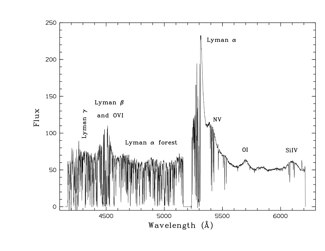
Figure 1: The complete Uves spectrum of Q 0103-260. The gap extending from 5164 Å to 5230 Å resulted from the space between the two CCDs of the Uves red arm CCD mosaic.

Since this investigation deals with the measurement of absorption features, some effort was devoted to determine a suitable and meaningful continuum level and to assess the accuracy of this function. As all absorption lines are very narrow compared to QSO emission features, we were not interested in the true (non-thermal and thermal) continuum emission of the quasar. Instead, we tried to derive the quasi-continuum formed by the superposition of the true continua and the broad emission lines and blends of the QSO. As this quasi-continuum is difficult to predict from models, it was determined empirically from local 5th-order polynomial fits through apparently line-free sections of the observed quasi-continuum. This procedure is relatively safe in the red spectral region, even at the position of broad emission lines (except at the peak of the Ly$\alpha$ emission line, which was omitted from the following analysis). However, due to the large number of Ly$\alpha$ absorbers, the assumed quasi-continuum blue-ward of the Ly$\alpha$ emission line peak depends somewhat on the subjective judgement of the reality of apparent continuum islands between the Ly forest lines. In order to estimate the uncertainties possibly introduced by this subjective judgement, we repeated the procedure of selecting the fulcrums and the subsequent interpolation 10 times. At positions where the quasi-continuum level appeared uncertain, we used, on purpose, different assumptions in the different runs. The 10 versions of the quasi-continuum were then averaged, and the variance between the different versions was used to estimate the accuracy of the continuum derivation. We found differences of the local continuum level derived in this way of up to 7% in the region of the Ly$\beta$, Ovi and Ly$\gamma$ emission lines. In most parts of the spectrum, however, the deviations were a few percent at most. Therefore, the uncertainties of the continuum level, while present, should not have influenced the statistical conclusions described in this paper. We also note that we checked for, but did not find any evidence for, a possible under-corrected zero-order contamination, as described by Rauch (1998), which could have influenced our measurements.

3 Line profile fits

Although the present study concerns mainly the investigation of the metal lines in the spectrum of Q 0103-260, it was important to first get some information on the Ly$\alpha$ absorption lines which form the great majority of the absorption features in the observed spectrum. According to Carswell et al. (1984), the profiles of typical Ly$\alpha$ lines in high-resolution (FWHM $<$ 25 km s^-1) QSO spectra can normally be approximated by Voigt profiles. Each line can hence be characterized by its Doppler parameter $b=\sqrt{2kTm^{-1}_{\mathrm{A}}+b^{2}_{\mathrm{turb}}}$, the column density $N_{\mathrm{HI}}$, and the redshift $z$.

The line profile $I(\lambda)$ for each line is then given by

$$I(\lambda)=I_{\mathrm{0}}\times{}e^{-\tau{}(\lambda)}$$ (1)

where the optical depth $\tau$($\lambda$) is

$$\tau{}(\lambda)=\frac{N_{\mathrm{HI}}r_{0}f{}\sqrt{\pi}c\lambda_{\mathrm{c}}10^{-8}}{b\sqrt{2\ln 2}}\times{}V(a,u)$$ (2)

and $V(a,u)$ is the Voigt profile function.

A powerful and convenient fit program for Ly forest lines is the code VPFIT which is based on the above assumptions and which has been developed by Carswell et al. (1984). It is available from (www.ast.cam.ac.uk/$\sim$rfc/vpfit.html). This program, which uses $N_{\mathrm{HI}}$, $b$, and $z$ as fit parameters and minimizes a suitable $\chi^{2}$ function of these parameters, was used throughout the present study.

The main application of VPFIT was the identification and fit of the Hi absorption lines in the region blue-ward of the Ly$\alpha$ emission. As a first approximation, all these lines were assumed to arise from hydrogen. Hence, the identified metal lines were also included in the fit. Since VPFIT works best with small data “chunks”, the spectrum was divided into 16 sections of roughly 40 Å overlapping by up to 5 Å. Each section was fitted separately.

Normally, following Kim et al. (2001), more lines should be added to an existing fit if $\chi^{2}_{\nu}$ $\geq$ 1.3. In some cases where regions contained either a saturated line or a multitude of very weak lines with column densities $N_{\mathrm{HI}}$ $<$ 10^12.5 cm^-2, $\chi^{2}_{\nu}$ had to remain greater than the 1.3 threshold. (Fixing this threshold obviously is to some extent arbitrary, and increasing the number of components normally improves the fit. There is, however, no guarantee that a better fit, i.e. a smaller $\chi^{2}_{\nu}$, is always physically “more correct”).

Tests with different continuum normalizations and with filters applied to the spectrum before the fitting procedure showed that the fit results for lines with $\sim 13.2<\log N_{\mathrm{HI}}<15.5$ are very robust against such differences in the data handling. For very weak lines ($\log N_{\mathrm{HI}}<12.8$) and for saturated lines, the fit results were found to depend on details of the data reduction. Thus, the results for such lines should be taken with care and anybody wishing to make use of our results on very weak or saturated lines should repeat the data reduction.

An example of the results of the line fitting procedure with VPFIT is given in Fig. 2.

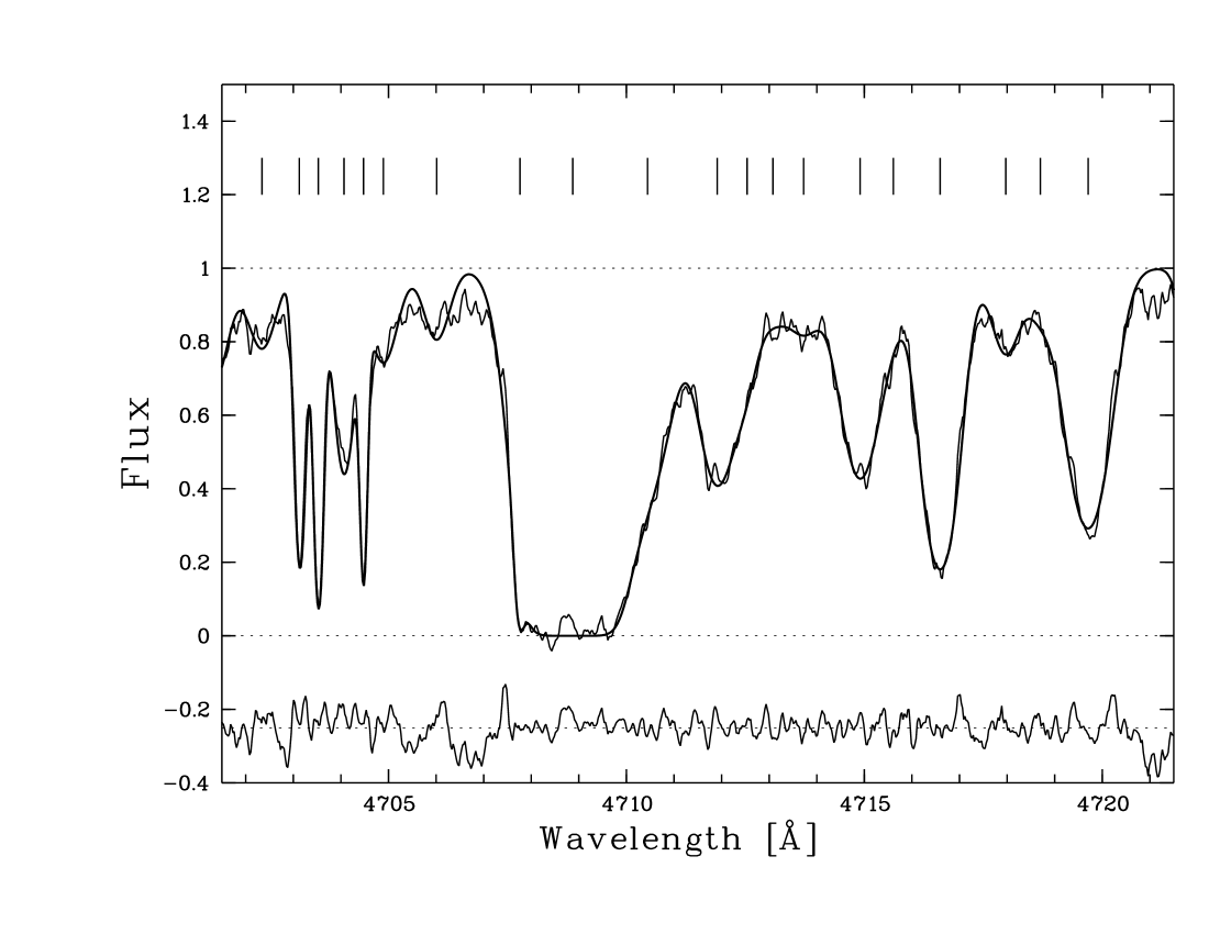
Figure 2: Example of the spectral fits obtained with VPFIT. The normalised observed spectrum and the model spectrum (smooth line) are plotted for a 20 Å section of the Lyman forest. Also plotted is the difference (for clarity downshifted by 0.25) between the fit and the data. The narrow lines at $\sim$ 4703 – 4705 Å are metal lines ( Siiv$\lambda$1394 at $z\sim$ 2.375 and Feii$\lambda$2383 at $z\sim$ 0.974). The tick marks above indicate the positions of the line centroids of the lines found by the fit procedure. For the saturated region near 4708 Å (where the fit is ambiguous, see text) assuming a blend of three lines gave the best result.

4 The Ly$\alpha$ forest lines

In order to verify that the intergalactic medium in the direction of the FDF has normal properties, we compared our new data with other Lyman forest studies of QSOs at similar redshifts. For this purpose, we calculated and compared various statistical quantities and functions, which are briefly described in the following paragraphs. To avoid confusion with the Ly$\beta$ forest, features caused by the strong Ovi lines, and the broad blends close to the Ly$\alpha$ emission peak, the Ly$\alpha$ forest analysis was restricted to the wavelength range from 4530 to 5165 Å. In this wavelength range the fit procedure resulted in the detection of 423 lines. Of these lines, 49 were removed from the sample because their small line widths ($b<$ 15 km s^-1) made an identification with metal absorption more likely, or because a too low ($N_{\mathrm{HI}}$ $<$ 10^12.5 cm^-2) or too high ($N_{\mathrm{HI}}$ $\geq$ 10¹⁶ cm^-2) column density made their analysis uncertain. Therefore, only 374 “reliable” lines were used in the following analysis of the Lyman forest. However, since the fraction of discarded lines is still small, the concentration on the “reliable” Hi lines should not have had any significant influence on the statistical results.

A plot of the Hi line fit from 4530 to 5165 Å as well as a line list derived from this fit is available on the web site http://www.astronomy.ohio-state.edu/$\sim$frank. The corresponding catalog lists the redshifts $z_{\mathrm{abs}}$, the column densities $N_{\mathrm{HI}}$, and the broadening parameters $b$ for the reliably measured Ly$\alpha$ absorption lines.

For the 374 lines selected in this way we investigated the following quantities and relations:

4.1 Column density distribution function

The column density distribution function (CDDF), $f(N_{\mathrm{HI}})$, measures the number of absorption lines per unit column density (in units of cm^-2) and per unit absorption path (defined as $x(z)=1/2\,[(1+z)^{2}-1.0]$ for $q_{0}=0.0$, which was adopted here primarily for the the reason of comparability to data sets by other authors) as a function of $N_{\mathrm{HI}}$. It is comparable to the luminosity function in the study of galaxies. For the CDDF of the Ly$\alpha$ forest of Q 0103-260 we find that the distribution can be well approximated by

$$f(N_{\mathrm{HI}})=7.1\times 10^{9}N_{\mathrm{H}}^{-1.62}$$

which is in good agreement with earlier results demonstrating that the CDDF can always be approximated by a power law with an exponent near $-1.5$ (Hu et al. 1995; Lu et al. 1996; Kim et al. 1997; Kirkman & Tytler 1997; Kim et al. 2001; Weymann et al. 1998; Lu et al. 1991).

4.2 Line number density

For the line number density, defined as

$$\frac{dN}{dz}=\left(\frac{dN}{dz}\right)_{\mathrm{0}}(1+z)^{\gamma}$$

where $dN$ is the number of lines per redshift range $dz$, $(\frac{dN}{dz})_{\mathrm{0}}$ is the local number density of the forest ($\approx 9.1\pm 0.4$), and $\gamma\approx 2.19\pm 0.27$, according to Kim et al. (2001), we find for $13.6<N_{\mathrm{HI}}<16.0$:

$$\log(\frac{dN}{dz})=2.27\pm 0.05$$

at a mean $z$ of 2.99, which falls exactly on the corresponding relation derived by Kim et al. (2001) for $z>1.5$.

4.3 Mean HI opacity

For the mean or effective Hi opacity $\tau_{\mathrm{eff}}$, defined as
$e^{-\tau_{\mathrm{eff}}}=<e^{-\tau}>$ (where $<>$ indicates averaging over the wavelength) we obtain for $z$ = 2.99 the value $0.36\pm 0.05$, which is again in excellent agreement with the results of Kim et al. (2001) and others.

4.4 Line counts

The number of lines in a given $z$ interval as a function of the flux threshold $F_{\mathrm{t}}$, and the number of lines as a function of the filling factor, defined as the fraction of the spectrum occupied by pixels whose normalized flux is smaller than a given flux threshold $F_{\mathrm{t}}$, again, were found to agree with the corresponding functions derived in earlier studies (Kim et al. 2001; Schaye et al. 1999; Outram 1999; Kirkman & Tytler 1997; Hu et al. 1995; Lu et al. 1996; Press et al. 1993).

4.5 Doppler parameter distribution and temperature-density relation

The distribution of the Doppler parameter $b$ for the Ly$\alpha$ lines can be well approximated by a Hui-Rutledge distribution (Hui & Rutledge 1999) with $b_{\mathrm{HR}}$ = 13.8 km s^-1 and $b_{\sigma}$ = ($23.7\pm 2.8$) km s^-1. In order to derive information on the temperature of the IGM, we investigated the relationship between the (baryon) density and the temperature $T$ by looking for a cut-off in the observed column density vs. Doppler parameter distribution.

The resulting temperatures of $\sim$ 15 000 – 20 000 K at the mean column density of $N_{\mathrm{HI}}$ = 1.9 $\times 10^{13}$ cm^-2 are in good agreement with photoionization models.

Table 2: Line list for the three metal line systems with redshifts close to that of the QSO emission lines. N denotes the minimum number of velocity components observed in the line profile. An asterisk in the last (Re) column points to a comment in Section 5.2. “bl” in this column indicates that the line is significantly blended.

$\lambda_{\mathrm{obs}}$	Ident		$z$	N	EW	m.e.	Re
(Å)					(Å)	(Å)
z3
4267.2	Ciii	977	3.367	4	$<$.67		bl
4506.8	Ovi	1032	3.367	4	$<$2.0		bl
4531.7	Ovi	1038	3.367	4	$<$2.0		bl
5269.3	Siiii	1207	3.367	4	$<$.68	.038	*
5410.4	Nv	1239	3.367	4	1.503	.032
5427.8	Nv	1243	3.367	4	1.222	.020
5827.9	Cii	1335	3.367	4	0.032	.015
6086.6	Siiv	1394	3.367		$<$0.05
6125.9	Siiv	1403	3.367		$<$0.05
z2
4262.8	Ciii	977	3.363	4	$<$2.6		bl
4318.5	Niii	990	3.363	7	0.329	.060
4502.4	Ovi	1032	3.363	7	$<$2.9		bl
4527.2	Ovi	1038	3.363	7	$<$3.8		bl
5264.1	Siiii	1207	3.363	7	1.190	.066
5405.1	Nv	1239	3.363	7	2.072	.057
5422.5	Nv	1243	3.363	7	1.444	.061
5422.6	Cii	1335	3.363		$<$.04
6081.1	Siiv	1394	3.363	7	1.280	.072
6120.3	Siiv	1403	3.363	7	0.906	.065
z1
4256.0	Ciii	977	3.356	4	0.920	.029
4494.9	Ovi	1032	3.356	5	$<$4.0		bl
4519.8	Ovi	1038	3.356	5	$<$4.2		bl
5255.6	Siiii	1207	3.356	5	0.460	.035
5396.4	Nv	1239	3.356	5	0.490	.042
5413.8	Nv	1243	3.356	5	0.290	.037
5813.2	Cii	1335	3.356		$<$.03
6071.2	Siiv	1394	3.356	5	0.430	.028
6110.5	Siiv	1403	3.356	5	0.290	.030

Table 3: Line list for the metal absorption line systems with $2.1<z<3.2$

$\lambda_{\mathrm{obs}}$	Ident		$z$	N	EW	m.e.	Re
(Å)					(Å)	(Å)
4300.5	Ovi	1038	3.145	2	0.045	.020	*
5134.6	Nv	1239	3.145	2	0.047	.021	*
5151.1	Nv	1243	3.145	2	0.041	.020	*
5531.2	Cii	1335	3.145	2	0.019	.020	*
5776.7	Siiv	1394	3.145	2	0.194	.029
5814.2	Siiv	1403	3.145	2	0.130	.025
4271.2	Ovi	1038	3.116	2	0.029	.020	*
4966.5	Siiii	1207	3.116	2	0.347	.035	*
5115.6	Nv	1242	3.116	2	0.021	.012	*
5737.3	Siiv	1394	3.116	2	0.154	.023
5774.4	Siiv	1403	3.116	2	0.120	.022
4557.4	Nv	1239	2.679	1	$<$0.04	0.015	*
5695.6	Civ	1548	2.679	1	0.105	.013	*
5705.0	Civ	1551	2.679	1	0.063	.013	*
5508.6	Civ	1548	2.558	1	0.268	.023
5517.8	Civ	1551	2.558	1	0.169	.022
4958.3	Siiv	1394	2.558	1	0.042	.020
5507.8	Civ	1548	2.558	1	0.155	.021
5517.0	Civ	1551	2.558	1	0.090	.013
4703.3	Siiv	1394	2.375	2	0.430	.030
4733.7	Siiv	1403	2.375	2	0.385	.040
5224.4	Civ	1548	2.375	2	0.350	.068	*
4330.6	Cii	1334	2.245	2	0.188	.010	*
4522.8	Siiv	1394	2.245	2	0.350	.020	*
4552.0	Siiv	1403	2.245	2	0.290	.015	*
4954.2	Siii	1527	2.245	2	0.068	.025	*
5023.9	Civ	1548	2.245	2	?		bl
5032.3	Civ	1551	2.245	2	?		bl
6018.6	Aliii	1855	2.245	2	0.109	.010
6044.8	Aliii	1863	2.245	2	0.045	.010
4329.6	Cii	1334	2.244	2	0.042	.014
4521.7	Siiv	1394	2.244	2	0.112	.020
4551.0	Siiv	1403	2.244	2	$<$.11		bl
5022.7	Civ	1548	2.244	2	$<$.19		bl
4421.8	Siiv	1394	2.173	1	0.133	.010
4450.5	Siiv	1403	2.173	1	0.095	.011
4911.8	Civ	1548	2.173	1	0.360	.020
5884.2	Aliii	1855	2.173	1	0.032	.015
5909.6	Aliii	1863	2.173	1	0.042	.016
4910.8	Civ	1548	2.172	1	0.180	.015	*
4919.0	Civ	1551	2.172	1	0.157	.016	*
4836.2	Civ	1548	2.124	1	0.168	.010
4844.2	Civ	1551	2.124	1	0.122	.012
5793.6	Aliii	1855	2.124	1	0.031	.019
5818.8	Aliii	1863	2.124	1	0.015	.015

Table 4: Line list for the two metal absorption line systems near $z$ = 0.974

$\lambda_{\mathrm{obs}}$	Ident		$z$	N	EW	m.e.	Re
(Å)					(Å)	(Å)
4688.1	Feii	2374	.9744	5	0.260	.080	bl
4704.5	Feii	2383	.9744	5	0.399	.030	bl
5107.0	Feii	2587	.9744	5	0.240	.035	bl
5133.7	Feii	2600	.9744	5	0.438	.030	bl
5521.1	Mgii	2796	.9744	5	1.080	.040
5535.2	Mgii	2804	.9744	5	0.880	.030
5632.8	Mgi	2853	.9744	5	0.235	.030
4626.8	Feii	2344	.9737	3	0.020	.030	bl
4702.9	Feii	2383	.9737	3	$<$0.130		*
5132.0	Feii	2600	.9737	3	0.026	.050
5519.2	Mgii	2796	.9737	3	0.229	.030
5533.4	Mgii	2804	.9737	3	0.120	.030
5631.9	Mgi	2853	.9737	3	0.030	.030

From the above comparisons we conclude that the Ly$\alpha$ forest of the FDF quasar has parameters which are rather typical for this redshift and that the IGM along the line of sight to Q 0103-260 has normal properties.

5 The metal lines

5.1 Line identifications

About 10 % of the absorption lines in the Uves spectrum belong to UV transitions of common ions of elements heavier than He in various ionization states. Following astrophysical traditions, all such lines are called “metal lines” in this paper. Except for very weak and very strong lines, the metal lines in the Uves spectrum are easily recognized on the basis of their lower line width (see e.g. Fig. 2). As suggested by Rauch et al. (1997b) we assumed all reasonably strong lines with $b<$ 15 km s^-1 to be metal lines. In order to assign these lines to certain atoms, ions, and redshifts, we used the following procedure: First, we identified the absorption lines connected with the QSO and its immediate environment. From earlier studies of the Fors Deep Field it is known that Q 0103-260 is embedded in an accumulation of bright starburst galaxies at nearly the same redshift (Heidt et al. 2003a). Hence, we expected (and found) strong absorption line systems superimposed on the quasar emission lines. Because of their association with the quasar emission lines and their known redshifts (within 0.01 of the emission line redshift) these lines could be readily identified independently of their width. In total we found three different groups of lines with $z\approx z_{\mathrm{QSO}}$. In Table 2 these redshift groups are labeled (in the order of increasing redshift) as z1, z2, and z3.

As a next step, we used our identified Ly$\alpha$ forest lines to look for metal emission at the redshifts of the strongest unblended Hi absorption lines. The rest wavelengths and expected line strengths of the metal lines were taken from the catalog of Morton (1992). For those narrow lines which were still unidentified after this step, we calculated mutual wavelength ratios which were compared with those expected for common Ly forest metal lines (making use of the fact that wavelength ratios are invariant to the redshift). At the high spectral resolution of Uves, this method is particularly powerful for identifying lines belonging to multiplets. For each line we then calculated the redshift. A metal absorption system was assumed to be established when at least 3 lines or blends (in some cases including an Hi line) were found to have redshifts not deviating by more than 0.0001. Having established a metal system in this way, we searched for other expected lines at the same redshift.

Using this procedure, we were able to identify more than 80 metal lines or blends belonging to 16 redshift systems. About 20 (mostly weak) sharp lines remained unidentified. Lines were assigned to the same redshift system if their profiles overlapped for at least one metal line. With few exceptions each system contains several components. In some cases an optimal line fit required the assumption of up to 16 components. However, as pointed out above, optimized line fits may overestimate the number of real components. Therefore, we determined for each system also a lower limit of components by counting the profile components which were directly visible on our spectra. The metal lines and blends, for which reliable observed wavelengths or equivalent widths could be measured, are listed in Tables 2 to 4. Lines and blends belonging to the same system are grouped together. In cases where only one component of a doublet is listed, the second component could not be measured because of blending. But in all these cases it has been verified that the spectrum is consistent with the presence of both components at the expected absorption strength ratio. The individual columns of the tables give the mean observed wavelength of the line (averaged over the individual velocity components), the line identification, the approximate mean redshift $z$, the lower limit of velocity components $N$, the total observed equivalent widths EW (derived by summing up the contributions of all individual velocity components), and their mean errors. An asterisk in the last column indicates a comment in the Subsection 5.2., whereas “bl” denotes blending with other lines (usually Hi). For some lines blending made it impossible to derive reliable equivalent widths. We then give as upper limits the EW which the line would have if the contribution of other lines were negligible. In addition to data for reliably detected lines, some upper limits or non-significant EW values have been included in the tables if these values provide information on line ratios important for the derivation of the ionization parameter or the plasma density. For many redshift systems, additional lines are visible in the Uves spectrum, but cannot be measured because of blending. This applies in particular to wavelengths below 4500 Å where the Ly$\alpha$ and Ly$\beta$ forests merge.

5.2 Remarks on individual metal absorption systems

$z$ = 3.367 (z3):

At least part of the absorption at the expected position of the Siiii resonance line seems to be due to Ly$\alpha$. Therefore, only an upper limit for the Siiii absorption can be given. Since Siiv is absent in this system, and since the strength of Ovi and Nv suggest a very high ionization parameter, a significant Siiii absorption is not to be expected, but cannot be ruled out by our observations.

$z$ = 3.145:

All metal lines of this system are weak. Only the lines of Siiv are significant detections.

$z$ = 3.116:

Weak Oiv and Nv and strong Siiii indicate a low ionization state. Cii, however, is not detected. Siiii could be overestimated due to blending with a weak Hi line.

$z$ = 2.679:

Except for the three lines listed, all lines coincide with regions of strong and complex blends.

$z$ = 2.375:

EW(Civ$\lambda$1548) has been measured in the Fors spectrum. Nv$\lambda$1243 is clearly detected, but not measurable because of too severe blending.

$z$ = 2.245:

The system consists of more than two (at least 3, possibly 7) components. The wavelength and EW values refer to the two strongest and best defined components only. The line ratios indicate a much lower ionization parameter than observed in the other systems.

$z$ = 2.172:

The only statistically significant metal lines are those of the Civ resonance doublet. Siiv is not detected, but the well defined sharp lines and the excellent agreement with the theoretical wavelength ratio makes it very likely that the identification of this weak system is correct.

$z$ = 0.9737:

The Feii$\lambda$2383 Å line could not be measured accurately because of an uncertain continuum level at the corresponding wavelength. The strong lines of low ionization stages indicate that the ionization parameter is much lower than in the systems with higher redshifts.

5.3 General properties of the observed metal systems

5.3.1 The metal absorbers with z${}_{\mathrm{abs}}\sim$z_em(QSO)

As mentioned above and listed in Table 2, there are three strong absorption systems with lines of Ciii, Niii, Nv, Ovi, Siiii, and Siiv, at redshifts close to the quasar’s emission line redshift ($z$ = 3.365, according to Noll 2002). Such systems with $z_{\mathrm{abs}}\approx z_{\mathrm{em}}$, which are observed in many quasar spectra, and are often referred to as the “intrinsic” absorbers, have been proposed in the literature to be either due to matter ejected from the QSOs or to originate in galaxies physically associated with the quasars. In a few cases evidence for a close association of such systems with the central QSO has been reported, e.g. time-variability of the line strength (Hamann et al. 1995) or partial coverage of the background source (Petitjean et al. 1994; Ganguly et al. 1999). In our case, the known accumulation of galaxies with about the same redshift around Q 0103-260 (e.g. Heidt et al. 2001) suggests that galaxies associated with the QSO at least contribute. On the other hand, of the three galaxies with reliable spectroscopic redshifts $z\approx z_{\mathrm{QSO}}$ and closer than 5 arcsec to the line of sight to the QSO only one (object 9003 in Noll 2002) has a redshift coinciding within the error limits with one of the systems listed in Table 3 (z3), while the two other galaxies have slightly larger (by 0.008–0.013) redshifts, indicating that they are located behind the QSO. However, there are additional faint galaxies close to the QSO without known spectroscopic redshifts, which could well cause the other $z\approx z_{\mathrm{QSO}}$ absorption systems.

For the system z3 we find a slightly (by about 0.002) higher redshift than derived for the QSO emission lines. However, as this difference is within the errors of the derivation of the emission line redshift, this result cannot be regarded as evidence for a motion of the absorbing gas towards the QSO.

In Figs. 3 and 4 the profiles of the three intrinsic absorption systems z1 to z3 and the corresponding spectral fits are presented. For these fits it was assumed that the same velocity components with exactly the same individual redshifts were present at all lines, while the absolute and relative strength of the components was allowed to vary from line to line. The wavelengths of the individual components are, if present, indicated in Figs. 3 and 4. A table of the fit parameters and the column densities derived from the fits is also available electronically from the web page noted above. It is evident from the plotted profiles that each system consists of discrete absorptions with different velocities and that the different velocity components have different strengths for different lines. As demonstrated by the figures and Table 2, all three systems show very strong high-ionization lines while significant absorption features of low-ionization stages (like the resonance lines of Cii, Nii, Siii, and Oi) were not detected. Siiv is fairly strong in z1 and z2, but not detected at z3. On the other hand, an absorption feature is present at the expected position of the Siiii line of the z3 system. However, the profile of this feature indicates that at least part (and possibly all) of this feature is due to Ly$\alpha$. A comparison with photoionization models (see e.g. Bergeron & Stasinska 1986; Steidel 1990; Songaila & Cowie 1996) indicates that the ionization parameter $\Gamma$ (while high for all three “intrinsic” systems) increases from z1 to z3. Hence, it appears likely that the apparent Siiii line of z3 is in fact due to Hi at a lower redshift and that Siiv (and lower Si ionization stages) have been destroyed by strong radiation short-ward of the He⁺ break.

Because of the relatively few significant line strength measurements our data do not allow to derive reliable quantitative values for the densities, ionization parameters and abundances in the observed metal systems. From the EW ratio Nv/Siiv it is clear, however, that the lines are formed in a plasma of relatively low density and a very high ionization parameter, and that the ionization parameter is decreasing with decreasing redshift. Such a behavior is to be expected if the redshift is related to the distance and if the QSO provides the ionizing radiation.

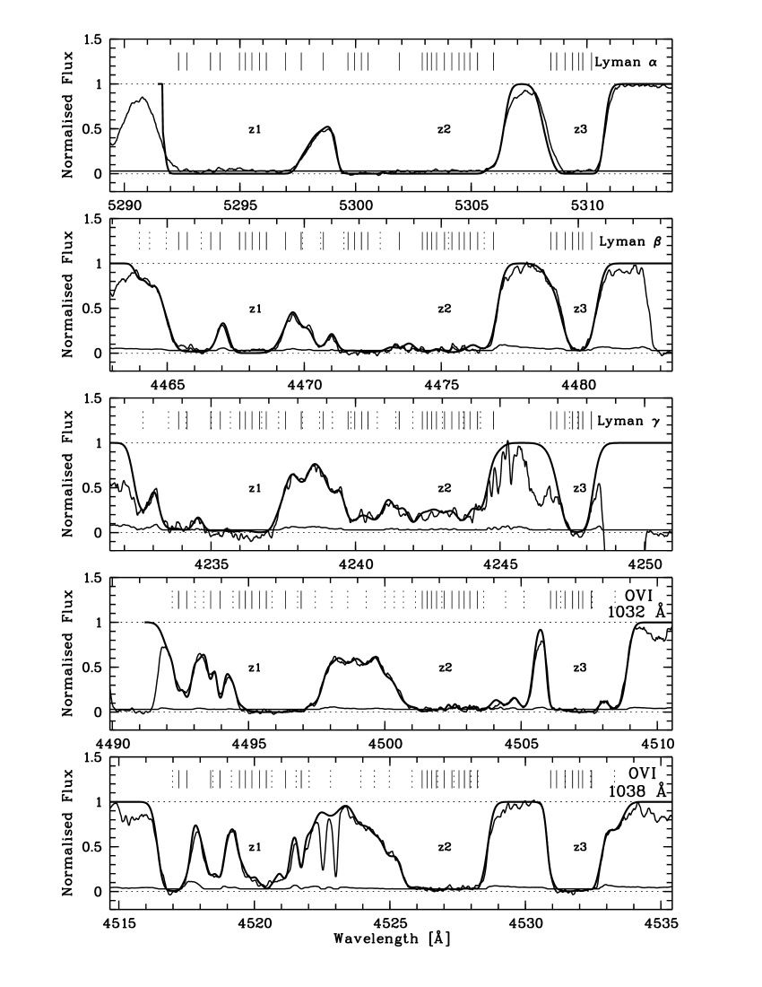
Figure 3: Line profiles of the blends produced by the metal absorption systems z1 to z3 with redshifts close to the quasar emission line redshift (thin line). Also included is the the model spectrum produced by the fit procedure (smooth thick line) and the mean error of the observed spectrum (thin line close to the zero level). The solid tick marks above the spectra indicate the centroids of the different line components assumed for the fit. Dashed tick marks represent the centroids of Hi at other redshifts added to obtain adequate fits. The relatively large residuals near Ly$\gamma$ are due to a detector defect (at 4249Å) and the omission of lower-$z$ Ly$\alpha$ lines in the fit.

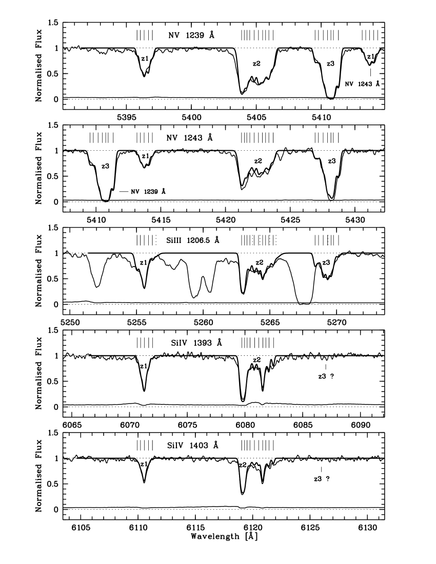
Figure 4: Line profiles of the blends produced by the metal absorption systems z1 to z3 with redshifts close to the quasar emission line redshift, continued. The Hi blends between the three Siiii features could not be fitted unambiguously and, therefore, were excluded from the fit.

5.3.2 The metal absorbers with 2.0 $<z<$ 3.2

Compared to the “intrinsic” systems all observed metal systems at lower redshifts have line ratios indicating lower ionization parameters. Most of these systems, though, are dominated by high-ionization lines too, with lines from neutral or single ionization stages not being detectable. Only one system ($z$ = 2.245) shows significant absorption by low-ionization lines.

The high state of ionization of the metal systems listed in Table 3 agrees well with the theoretical predictions of Rauch et al. (1997a) and Haehnelt (1997) who used hydrodynamic computations to calculate the spatial distribution and line absorption of low-metallicity intergalactic gas at high redshift. From a detailed comparison of the relative line strengths in Table 3 with the calculated column densities of Rauch et al. (1997a), we find the high-ionization lines (such as Ovi, Nv, Civ) to follow the predictions rather well. The theoretical results of Rauch et al. (1997a) also provide a plausible explanation for the weakness of absorption lines of low ionization species such as Cii, which are expected to be present only in the rare cases where the line-of-sight passes through a high density core of a protogalactic clump of the intergalactic gas.

The agreement with the predictions of Rauch et al. (1997a) is less good for species with intermediate ionization potentials. In particular, we find the Siiv and Siiii lines listed in Table 3 to be on average stronger and the resulting Siiv/Civ and Siiv/Nv column density ratios about 10 times higher than predicted for a metal-poor gas with a solar relative composition. As in the case of the measurements of Songaila & Cowie (1996), the discrepancy is smaller if our data are compared to the calculations made assuming the chemical composition of galactic metal-poor stars. But even in this case, our Siiv lines are on average too strong by about a factor of 4.

A comparison with Misawa et al. (2002) indicates that the observed number density of Civ systems with EW $>$ 0.15 Å in the redshift range $2.1<z<3.2$ along the line-of-sight to Q 0103-260 is normal for a QSO at this redshift. Although additional systems with smaller EW values are present in Table 3, our data provide no evidence for a high abundance of weak metal systems.

5.3.3 The Mg/Feii systems at $z\approx 0.974$

While there are several sharp lines in the red part of the spectrum which are suspected to be due to low-ionization lines at moderate redshifts, only two metal systems with redshifts $<$ 2 could be reliably identified. The profiles of the strongest lines of these two systems with almost identical redshifts ($z\approx$ 0.974) are presented in Fig. 5. Both systems consist of various components and show a complex structure. The plasma producing these lines has a relatively low ionization level, comparable to that of most of the interstellar matter in our galaxy and the gas observed in low-$z$ metal absorption systems (see e.g. Bergeron & Boissé 1991).

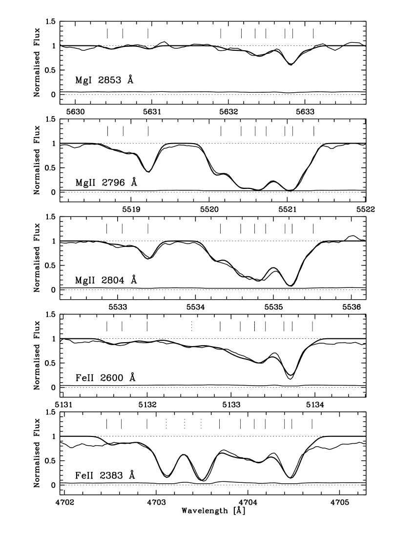
Figure 5: The two Mg/Feii absorption systems at $z\approx 0.974$. Also plotted is the model spectrum (thick smooth line). The tick marks again indicate the positions of the centroids of the lines assumed for the fit. The two strong absorption lines at 4703.1 Å and 4703.5 Å in bottom panel are due to Siiv$\lambda$1394 at $z$ = 2.375.

6 Correlations

Because of the relatively small observed Ly$\alpha$ redshift range and the presence of the superimposed metal lines, the distribution of the Ly$\alpha$ absorption-line redshifts provides only limited information on the cosmic structure along the line-of-sight to the observed quasar. In particular, we found for the redshift range 2.7 $<$ z $<$ 3.3, where we have the most reliable data on the Ly$\alpha$ absorption, a number density distribution of the Ly$\alpha$ lines which is almost fully consistent with a random distribution of the absorbers along the LOS. A clustering signal could be detected only for the two-point correlation function in the lowest velocity range ($\Delta v\leq$ 50 km s^-1) and in the step optical depth function (Cen et al. 1998) for velocity separations $\sim$ 5–10 km s^-1. The clustering signal is higher for the systems with higher column density. This result is in good agreement with earlier reports on the clustering of Lyman forest lines on small scales (see e.g. Webb 1987; Hu et al. 1995; Lu et al. 1996; Chernomordik 1995; Cristiani et al. 1995, 1997). However, while little structure is evident in the number density distribution of the Ly$\alpha$ absorbers, structure is indicated in the total Hi absorption as a function of redshift (cf. Fig. 7). More specifically, we find an absence of high column density absorption and a lower-than-average total Ly$\alpha$ absorption in the redshift interval $2.8<z<3.1$.

More interesting information on the distribution and the properties of the absorbing gas along the LOS to Q 0103-260 is provided by the redshift distribution of the metal-line systems and by a comparison of this distribution with the galaxy redshift distribution in the FDF. From Tables 2 to 4 it is obvious that the metal absorption systems also tend to cluster on small scales. Moreover, no metal absorption system is detected in the redshift range $2.8<z<3.1$ where the Ly$\alpha$ absorption is weak. A comparison between the redshifts of the individual metal absorption systems and those of the Ly$\alpha$ absorption lines shows that (as expected) detected metal line systems always correspond to strong Ly$\alpha$ absorption. On the other hand, there are strong Ly$\alpha$ absorption features without detectable corresponding metal absorption. A notable example is the Ly$\alpha$ absorption at $z$ = 2.758. The total Ly$\alpha$ absorption of this system is similar to or slightly stronger than that for the two systems at $z$ = 2.558, but no metal absorption is detectable. The upper limits for the Civ and Siiv absorption are by factors of at least 0.05 to 0.1 lower than the corresponding metal line strengths in the $z$ = 2.558 systems. We regard these large differences as clear evidence for strong local variations of the metal enrichment at this redshift.

The existence of photometric and spectroscopic redshifts for a significant fraction of the FDF galaxies allows us to compare the redshift distributions of the galaxies with those of the absorption line systems discussed here. At present photometric redshifts are known for about 6500 FDF galaxies (Bender et al. 2001; Gabasch et al. 2003) while so far (accurate) spectroscopic redshifts are available for only about 270 galaxies (Noll 2002; Noll et al. 2003). Some properties of the QSO absorption line distribution (such as the lower-than-average density of objects at $2.8<z<3.1$ and an over-density near the redshift of Q 0103-260) are also indicated in the distribution of the galaxy’s photometric redshifts. However, the accuracy of photometric redshifts is much lower than that of the Uves absorption line redshifts and generally too low for a meaningful detailed comparison. The available spectroscopic galaxy redshifts (m.e. about 0.002) is adequate for the present purpose, but the number of available redshifts is uncomfortably small for statistical purposes. Fortunately, the FDF spectroscopic observing program is biassed towards high redshift objects. Therefore, for the redshift range $2.0<z<3.4$, corresponding to (most of) the metal line redshifts in this investigation, the present spectroscopic catalog is $\approx$ 50 % complete for a limiting I-Magnitude of 24.0. At least for this $z$ range the present spectroscopic redshift catalog can be regarded as representative sample which can be used for the present statistical purposes.

Fig. 6 presents a histogram of the $z$ distribution of the presently available accurate spectroscopic redshifts $2.0<z<3.7$ in the FDF. Also indicated in this figure are the redshifts of the metal absorption systems of Q 0103-260 (broken vertical lines) in this range. In order to avoid meaningless small numbers and in view of the expected peculiar velocities of the galaxies, we used histogram bins of $\Delta z=0.01$. If the redshifts of the 77 galaxies included in Fig. 6 were distributed randomly we would have to expect on average 0.45 objects per bin and a Poisson distribution of the actual number of objects per bin. While the population of most bins is roughly consistent with this assumption, various bins show highly significant (corresponding to 3 to 6 $\sigma$) deviations. In particular, the clustering of galaxy redshifts at the $z$ values 2.245, 2.34, 2.37, 2.48, 3.14 and 3.38 cannot be explained by statistical fluctuations of a random distribution. Also statistically significant is the total absence of objects with redshifts $2.78<z<3.03$. Such strong deviations from a random distribution of the galaxy redshifts, which have been found and discussed before in the context of other deep fields (see e.g. Cohen et al. 1996; Steidel et al. 1998; Giavalisco 2002) are obviously the result of the cosmic large-scale structure. In most cases the galaxies included in a single redshift bin are distributed over the whole FOV of the FDF. In general, the velocity dispersion in the redshift clumps relative to the (minimum) observed size of these structures are too large to form bound systems, although in some bins (such as in the strong peak near $z$ = 2.37) many objects have the same redshift within the error limits, making it likely that these accumulations are or are becoming bound and are precursors of galaxy clusters.

As shown by Fig. 6, 13 of the 16 metal system redshifts coincide with populated galaxy redshift bins. In the absence of a correlation (i.e. assuming random distributions) less than 4 such coincidences are expected to occur. Hence, Fig. 6 provides not only strong evidence for the presence of large-scale structure in the galaxy redshift distribution, but also for a strong correlation of the galaxy distribution and the metal absorbers which obviously trace the same large-scale structure. The fact that no galaxies have been found at the redshifts of the metal absorptions system with redshift 3.116 and the two adjacent systems near $z$ = 2.558 can readily be explained by the incompleteness of our spectroscopic survey. More interesting is the fact that for the conspicuous clustering of galaxy redshifts near $z$ = 2.34, in spite of a thorough search at the expected wavelengths, no trace of corresponding metal absorption systems could be detected. Whether Ly$\alpha$ absorption is present at this redshift, cannot be tested with our data since the corresponding wavelength is outside our Uves spectrum. Interestingly, the galaxies belonging to this clustering differ from the other redshift groups by a pronounced clustering tendency on the sky, with the center of their distribution about 2 arcmin off the LOS to the QSO.

For the small spectral range, where simultaneous information on the Ly$\alpha$ lines, the metal lines, and the galaxy redshift distribution is available, we have included the data for all three components in Fig. 7. For this purpose, the Uves spectrum has been smoothed to a redshift resolution of 0.005 to be comparable with the resolution of the galaxy redshifts. Moreover, the Uves spectrum has been normalized to the likely continuum level in the unsmoothed spectrum. The histogram of the galaxy redshift distribution has been scaled by a factor 0.1. The figure clearly shows the lower-than-average Ly$\alpha$ absorption and the absence of metal line systems and galaxy redshifts in the $z$ interval $2.80<z<3.05$ (corresponding to a comoving distance of about 300 Mpc). It is also interesting to note that the strong Ly$\alpha$ absorption near $z$ = 2.76 (which does not show corresponding metal absorption), while not exactly coinciding with the redshift of a galaxy spectrum, nevertheless falls into a redshift region where galaxies are observed.

We also checked our data for evidence of the weakening of Ly$\alpha$ absorption at the redshift of starburst galaxies close to the LOS reported by Adelberger et al. (2003). Although some of our foreground galaxies are close enough to potentially produce such an effect, our numbers are too small to provide reliable conclusions on this question.

As noted above, only two metal systems with (almost identical) redshifts $<2.0$ could be reliably identified in our Uves spectrum. Fig. 8 shows the distribution of the presently available spectroscopic redshifts and the position of the two (on this scale coinciding) metal system redshifts. When interpreting Fig. 8, one has to keep in mind that (in contrast to Fig. 6) the overall redshift distribution in Fig. 8 is strongly affected by an observational (negative) bias affecting galaxies in the redshift range 1.2 – 2.0 (cf. Noll 2002). On the other hand, the small scale structure of the redshift distribution in Fig. 8 should be representative. As illustrated in Fig. 8, the redshifts of the two detected low-$z$ systems again coincide with a clustering of galaxy redshifts. However, the plot also shows that there are many other such clusterings at low redshifts for which no absorption lines were detected. A reason that just the systems at $z=0.974$ are observed could be the fact that some galaxies with this redshift are exceptionally close to the line of sight to Q 0103-260. One galaxy falling into the corresponding redshift bin (No. 4442 in the catalog of Heidt et al. 2003b) has an angular distance of only about 11$\arcsec$. While it still appears unlikely that gas of this galaxy is responsible for the observed metal absorption, there are several galaxies with similar photometric redshifts (but no spectroscopic data) even closer to the LOS to the QSO, which may be associated with FDF 4442. These galaxies appear to be relatively normal late-type galaxies which could well produce the observed redshifted interstellar absorption features.

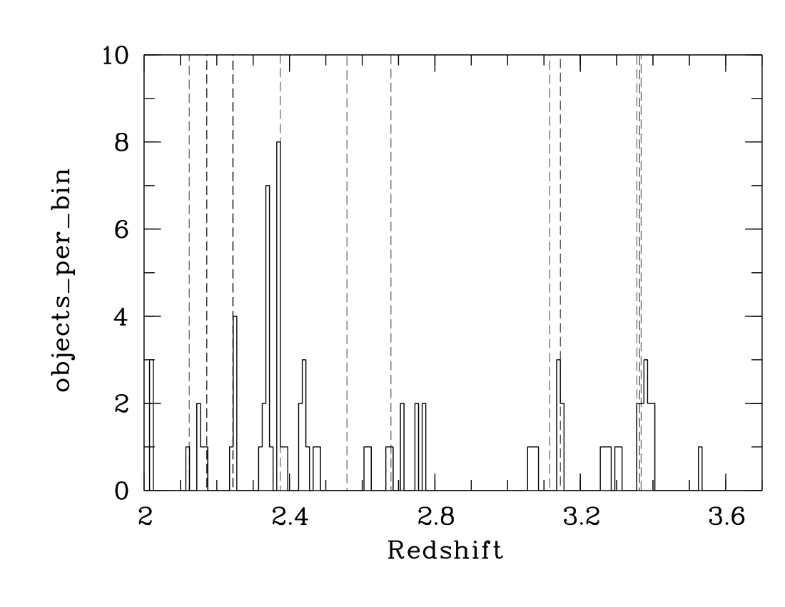
Figure 6: The redshift distribution of FDF galaxies with accurate spectroscopic redshifts in the range $2.0<z<3.7$. The broken vertical lines indicate the redshift positions of the metal absorption systems falling into this range. Note that the close groups of metal systems near the redshifts 2.172, 2.244, and 2.558 (cf. Table 3) are not resolved on this scale and appear as single systems in this figure.

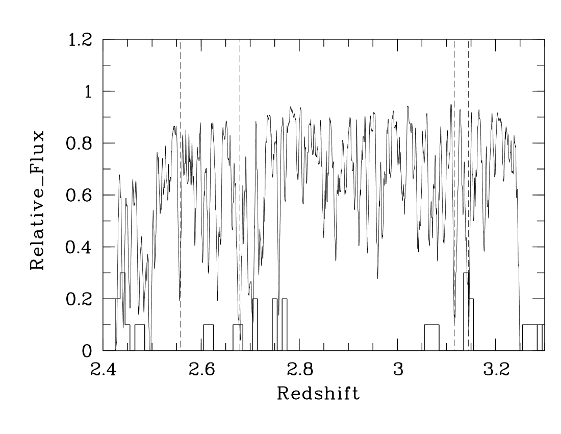
Figure 7: The normalized flux in the QSO spectrum showing the strength of the Ly$\alpha$ absorption as a function of redshift. Also given are the redshift positions of the metal absorption systems in this redshift range (vertical broken lines) and the histogram of the redshift distribution of the FDF galaxies (scaled by a factor of 0.1). For this figure the Uves spectrum has been smoothed to a resolution of $\Delta z=0.005$. It has been normalized to the continuum level of the unsmoothed spectrum. Note that the strong broad absorption features at $z$ = 2.70 and 2.72 are in fact due to Ovi absorption at $z$ = 3.36. The Ly$\alpha$ absorption at 2.68 is contaminated by Ly$\beta$ at $z$ = 3.36 and Ly$\gamma$ of this redshift contributes to the feature at 2.49. Most other strong features are due to Ly$\alpha$.

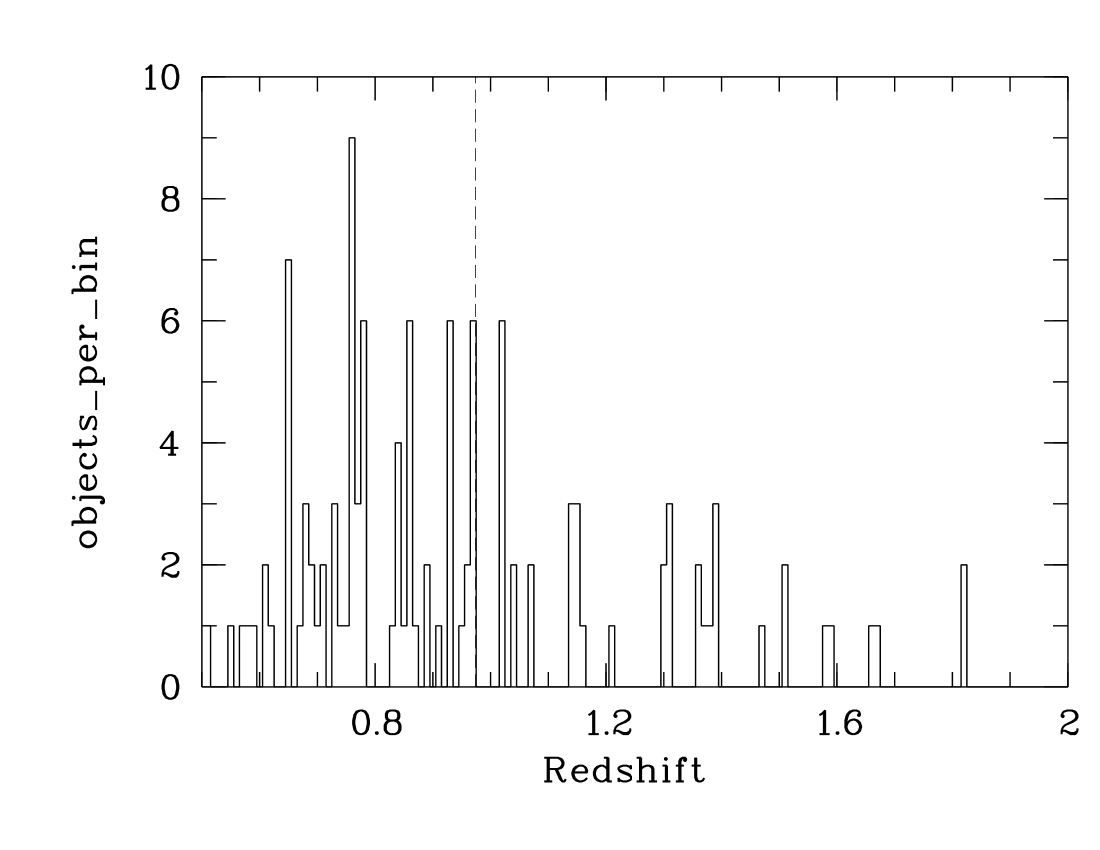
Figure 8: Distribution of spectroscopic galaxy redshifts in the FDF for $0.5<z<2.0$. The relatively low frequency of objects between 1.0 and 2.0 is due to an observational selection effect. The vertical broken line indicates the position of the $z=0.974$ Feii/Mgi/Mgii absorption system described in the text.

7 Conclusions

Our analysis of the absorption lines of the quasar Q 0103-260 and a comparison with spectroscopic redshifts of FDF galaxies confirm that the absorbers’ redshift distribution traces well a common large scale structure. The fact that the number density of the Ly$\alpha$ lines shows no significant deviation from a random distribution in the observed redshift range, while the total Hi absorption shows variations, seems to indicate that the Ly forest clouds in the region investigated show systematic local variations either of their density or of their ionization level, correlated with the galaxy density. The presence of Ly$\alpha$ clouds of high neutral Hi column densities in the FDF region is found to be highly correlated with strong metal line absorption and the presence of starburst galaxies at the same redshift. This obviously suggests that hydrogen clouds with high neutral column densities are (or have been) places of early vigorous star formation and the enrichment of the corresponding clouds with heavy elements. In agreement with other authors, we find large variations in the metal line strengths and ionization parameters of individual Ly$\alpha$ absorbers. At the same total Ly$\alpha$ absorption strength some clouds have strong metal lines while others show no trace of any metal absorption. Further studies of larger samples will be needed to determine the physical cause of these differences.