First Detection of Polarization of the Submillimetre Diffuse Galactic Dust Emission by Archeops

We present the first determination of the Galactic polarized emission at 353 GHz by Archeops. The data were taken during the Arctic night of February 7, 2002 after the balloon–borne instrument was launched by CNES from the Swedish Esrange base near Kiruna. In addition to the 143 GHz and 217 GHz frequency bands dedicated to CMB studies, Archeops had one 545 GHz and six 353 GHz bolometers mounted in three polarization sensitive pairs that were used for Galactic foreground studies. We present maps of the $I,\leavevmode\nobreak\ Q,\leavevmode\nobreak\ U$ Stokes parameters over 17 % of the sky and with a 13 arcmin resolution at 353 GHz ($850\leavevmode\nobreak\ \mu\mathrm{m}$). They show a significant Galactic large scale polarized emission coherent on the longitude ranges [100, 120] and [180, 200] deg. with a degree of polarization at the level of 4–5 %, in agreement with expectations from starlight polarization measurements. Some regions in the Galactic plane (Gem OB1, Cassiopeia) show an even stronger degree of polarization in the range 10–20 %. Those findings provide strong evidence for a powerful grain alignment mechanism throughout the interstellar medium and a coherent magnetic field coplanar to the Galactic plane. This magnetic field pervades even some dense clouds. Extrapolated to high Galactic latitude, these results indicate that interstellar dust polarized emission is the major foreground for PLANCK–HFI CMB polarization measurement.

1 Introduction

The power spectrum of the temperature anisotropies of the Cosmic Microwave Background (CMB) have now been measured over most of the relevant angular scales (10 arcmin to 90 deg, see a comparison of different experiments in e.g. Benoît et al. 2003a and Bennett et al. (2003)). However, CMB polarization is only in its experimental infancy. Theoretical predictions are rather tight for the polarization effect coming from the last scattering surface. Accurate polarization measurements are not only useful for breaking some degeneracies between cosmological parameters but also for obtaining the gravitationnal wave background. Upper limits on polarization (Keating et al. (2001); de Oliveira-Costa et al. (2003)) are now superseded by detections by DASI (Kovac et al. (2002)) and WMAP (Kogut et al. (2003)). New results can be expected from BOOMERanG, MAXIPOL and other experiments and later from Planck. For high frequency CMB measurements the most important foreground is certainly the emission from Galactic Interstellar Dust (ISD). Submillimetre and millimetre (hereafter submm) emission intensity of ISD can be inferred from IRAS and COBE–DIRBE extrapolations (e.g. Schlegel et al. (1998)) and has been measured on large scales by COBE–FIRAS (Reach et al. (1995); Boulanger et al. (1996); Lagache et al. (1998)). On the other hand, nothing is known on ISD polarization in emission on scales larger than 10 arcmin., i.e. those precise scales which are the most relevant for CMB studies. It is likely that ISD polarized emission is the major foreground for high frequency CMB polarization measurements. Ground–based observations of submm ISD polarization are concentrated on high angular resolution (arcminute scale) of star formation regions. Indirect evidence for large scale polarization come from the polarization of starlight in absorption (Fosalba et al. (2002)). Goodman (1996) gives a review of the measurements and ambiguities in the interpretation of the background starlight polarization. In particular, the visible data are biased by low column density lines of sight and do not fairly sample more heavily reddened ones. Direct submm measurements are therefore highly required both for Galactic studies of the large scale coherence of the magnetic field and in the field of CMB polarization, but are rather challenging as they require sensitivities comparable to those of CMB studies.

Archeops is an experiment designed to obtain a large sky coverage in a single balloon flight. First results on CMB anisotropies power spectrum are reported in (Benoît et al. 2003a ; Benoît et al. 2003b ). Here, we present the first results on ISD polarization measurements with Archeops. Its large sky coverage strategy is optimized for finding fairly strongly polarized sources without any bias on their location.

Section 2 briefly describes the instrument and Sect. 3 the ground based calibrations on polarized channels. Section 4 presents the specific processing applied to the polarized data. More specifically subsect. 4.5 presents the inversion method applied to determine the Stokes parameters. Section 5 is dedicated to the main results on local clouds and diffuse regions. Section 6 assesses the reliability of the results and Sect.7 their physical interpretation.

2 Description of the instrument

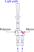
Figure 1: a) Scheme of an OMT at 353 GHz used for Archeops. The back to back horn is heat sunk to the 10 K stage. The box containing the polarizer beam splitter and the mirror is on the 1.6 K stage. The bolometers on the 100 mK stage and their associated horns are not shown. The light enters from the top of the drawing into the back to back horn (one horn per pair of bolometers). One polarization mode is transmitted through the polarizer beam splitter to the first bolometer (A, $\parallel$), the second mode is reflected to the second bolometer (B, $\perp$). This system ensures that each bolometer of the same pair sees the same point of the sky at the same time. b) Orientation of the polarization for each bolometer of the three OMTs in the focal plane. The arrow represents the scan direction. The thick solid lines refer to the $\parallel$ direction, the thick dashed lines refer to the $\perp$ direction.

A detailed description of the instrument technical and inflight performance is given in (Benoît et al. (2002), Benoît et al. 2003c ); we here provide only a summary description. Archeops is a balloon–borne experiment with a 1.5 m off–axis Gregorian telescope described in (Hanany & Marrone (2002)). In particular, it satisfies the Mizuguchi-Dragone condition (Mizuguchi et al. (1978); Dragone (1982)) in which there is negligible cross polarization at the center of the field of view. The cryostat contains a bolometric array of 21 photometers operating at frequency bands centered at 143 GHz (6 bolometers), 217 GHz (8), 353 GHz (6$\leavevmode\nobreak\ =$ 3 polarized pairs) and 545 GHz (1). The focal plane is maintained at a temperature of $\sim 100$ mK using a ³He-⁴He dilution cryostat. Observations are carried out by rotating the payload at 2 rpm producing circular scans at a fixed elevation of $\sim 41^{\circ}$. Pointing reconstruction is done a posteriori by using a dedicated optical stellar sensor made of a 40 cm optical telescope and 46 photodiodes. Observations of a single night cover a large fraction of the sky as the circular scans drift across the sky due to the rotation of the Earth. The experiment was launched on February 7, 2002 by the CNES from the Swedish balloon base in Esrange, near Kiruna, Sweden, $68^{\circ}$N, $20^{\circ}$E. It reached a float altitude of $\sim 34$ km and landed 21.5 hours later in Siberia near Noril’sk, where it was recovered by a Franco-Russian team. The night–time scientific observations span 12 hours of integration from 15.0 UT to 3.0 UT the next day. The polarized channels comprise of three quasi-optical modules, which are equivalent to Ortho Mode Transducers (hereafter OMT, Bøifot et al. (1990), Chattopadhyay & Carlstrom (1999)). A pair of conjugated bolometers (see Fig. 1) is coupled to the sky through a single 10 K back to back horn via the OMT. The OMT, which is attached to the 1.6 K stage, is made from a single polarizing grid mounted at 45 degrees to the horn axis to divide the incoming light into the two orthogonal polarization modes. One is transmitted to the first bolometer (A), the other is reflected towards the second one (B). At any time, the sum of the two bolometer outputs measures the total intensity while the difference measures the $Q$ Stokes parameters in the OMT eigen basis. The three OMT units are aligned along the scan direction and have their (A)–polarization axis oriented at $60^{\circ}$ with respect to each other in order to minimize errors in polarization reconstruction (Couchot et al. (1999)) (see Fig. 1).

3 Ground–based calibration

Laboratory measurements were performed in order to calibrate the transmission and orientations of the polarizers. The cross polarization of a single grid was measured to be less than 1 % and is neglected hereafter.

If $\tau$ is the intensity transmission rate and if $\parallel$ ($\perp$) refers to the transmitting (extinguishing) direction of a polarizer, then $K=(\tau_{\parallel}+\tau_{\perp})/2$, $k=(\tau_{\parallel}-\tau_{\perp})/2$ and $q=\sqrt{\tau_{\parallel}\tau_{\perp}}$ are the three parameters characterizing a polarizer in Stokes formalism. For an ideal polarizer, $K=0.5$, $k=0.5$, $q=0$. If ${\bf S}=(I,Q,U)$ is defined with respect to the observation basis $(x,y)$ and describes the polarization state of the radiation propagating along $-z$, and if the $\parallel$ direction of the polarizer makes an angle $\alpha$ with $x$, then the transmitted Stokes vector is ${\bf S^{\prime}}={\cal M}{\bf S}$, with the Mueller matrix being

$${\cal M}=\left(\begin{array}[]{ccc}K&k\cos 2\alpha&k\sin 2\alpha\\ k\cos 2\alpha&K\cos^{2}2\alpha+q\sin^{2}2\alpha&(K-q)\cos 2\alpha\sin 2\alpha\\ k\sin 2\alpha&(K-q)\cos 2\alpha\sin 2\alpha&K\sin^{2}2\alpha+q\cos^{2}2\alpha\end{array}\right).$$

In case of an unpolarized incoming radiation $I_{0}$, a photometer placed behind a polarizer receives $KI_{0}$. When it is placed behind two polarizers that are oriented at angles $\alpha$ and $\varphi$, it receives $(K_{1}K_{2}+k_{1}k_{2}\cos 2\alpha\cos 2\varphi+k_{1}k_{2}\sin 2\alpha\sin 2\varphi)I_{0}$. In the case of the 353 GHz bolometers, the OMT polarizer is fixed in the focal plane with an angle $\varphi$. Rotating a calibration polarizer (hereafter CP) in front of it and fitting the measured intensity as a function of $\alpha$ gives $k_{1}k_{2}\cos 2\varphi$ and $k_{1}k_{2}\sin 2\varphi$ from which $\varphi$ can be deduced.

We place a box containing a calibration polarizer which rotates at 1.5 rpm above the entrance window of the cryostat. The is covered with eccosorb to avoid parasitic reflections. It has two apertures. In one aperture we place a 77 K thermal source made of polystyrene cup filled with liquid nitrogen. The bottom of the cup is lined with eccosorb. The other aperture faces the cryostat. The black body emission is chopped at 13.4 Hz against the ambient temperature to enable lock-in detection. This set up allows us to determine the position of the grid polarizers in the OMT (see Fig. 1) to within 3 degrees. This source of error contributes an uncertainty of less than 5 % in $Q$ and $U$.

During the ground based preparation of the flight, we placed a matrix of $4\times 4$ grids of $50\leavevmode\nobreak\ \mu$m Cu/Be wires with a step of $100\leavevmode\nobreak\ \mu$m in front of the $1\;\mathrm{m}^{2}$ 2 Hz modulated thermal source (Benoît et al. (2002)) placed on a hill at $\simeq 1$ km from the telescope. This provided a linearly polarized blackbody source for an additional pre-flight polarization calibration. We verified that the orientation of the grid polarizers in the OMT agreed with the laboratory measurements and found that the beam shape in the $Q$ and $U$ states agreed with the $I$ beam shape within 20%.

4 Polarization data processing

4.1 Standard processing

The Stokes parameters reconstruction, as well as the cross–calibration described above, only apply to clean data associated with an accurate pointing. We here summarize the preparation of the data described in more details in (Benoît et al. 2003d ).

Pointing reconstruction is performed with about 200 detected stars per revolution and provides an rms pointing accuracy better than 1.5 arcmin. The polarizers angles determined from ground calibrations (see Sect. 3) can then be computed on the sky.

The raw Time Ordered Information (TOI), sampled at $\simeq 153$ Hz, are decompressed, then filtered to take into account the AC biasing scheme coming from the readout electronics. Cosmic rays, electronic spikes, artifacts and noisy data are detected and flagged with an automatic algorithm followed by visual inspection. Small areas around strong point sources are flagged as well. The flagged data representing less than 1.5% of the data are replaced by a constrained realisation of noise for subsequent detrending and high–pass filtering. The data are corrected with a bolometer model for drifts of the instrument response due to changes in the background optical loading and in the focal plane temperature. Low frequency drifts due to airmass and temperature fluctuations of the various stages of the cryostat (0.1 K, 1.6 K, 10 K) are decorrelated using housekeeping data (altitude, elevation, temperatures). A spin–synchronous atmospheric signal remains and prevents us from using the Cosmological Dipole for an accurate calibration. In–flight observations of Jupiter lead to the determination of the bolometer time constant (used to deconvolve the data stream) as well as the photometric pixel beams (with an error less than 10 %). The beams are identical within polarizer pairs and moderately elliptical, with a minor and major axis FWHM of resp. 10.6 and 13.4 arcmin. We assume that in–flight $Q,\;U$ beams are identical to the intensity beam.

4.2 Filtering

We briefly describe here the specific post–processing applied to the 353 GHz channels. This processing is not specific to polarization but rather to Galactic studies for experiments that have a scan strategy like Archeops or Planck.

The major noise component that remains after the pipeline (as described above) is some low frequency noise. A brute force low pass filter applied on the timeline generates ringing on both sides of the Galactic plane. The key issue is thus to remove the best low frequency baseline without producing a significant ringing. To do this, we first mask the Galaxy using a SFD template (Schlegel et al. (1998)) and use localized slowly varying functions (Benoît et al. 2003c ) to interpolate the Galactic plane and obtain a first estimation of the baseline. This estimation is used to perform a noise constrained realization of the timeline on the masked area. Then, an optimized low frequency baseline is calculated using wavelet shrinkage techniques (Macías–Pérez (2003)) which allow to remove high frequency noise. This baseline is subtracted from the original timeline.

4.3 Cross–calibration method

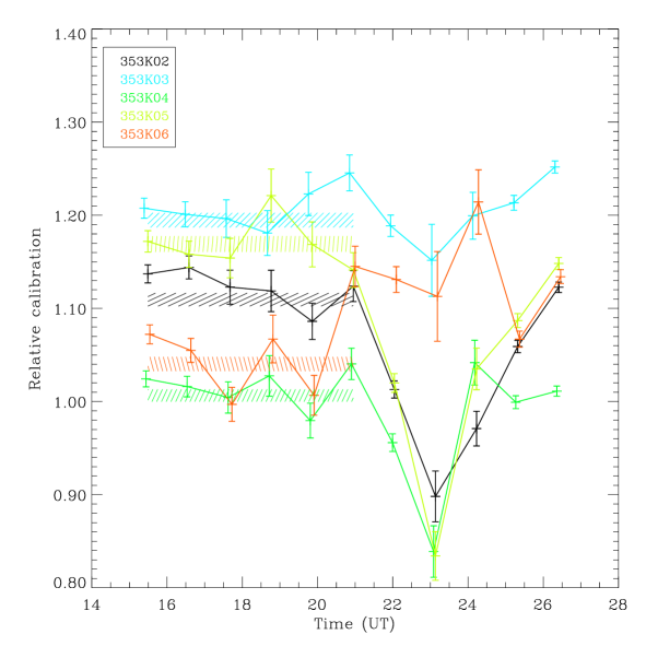
Figure 2: Variation of the cross–calibration coefficients $\alpha$ during the flight relative to the reference baolometer 353K01. The coefficients are mostly constant at the beginning of the flight (within error bars), but become noisier after UT=21h30. The shaded areas show the $\pm 1\sigma$ values of the coefficients used in the present analysis, and the time interval over which they are computed.

Since polarization is obtained from differences of measurements from detectors at various orientations, it is critical that they all be accurately cross–calibrated. Any mismatch in this cross–calibration automatically generates intensity leaks into the fainter polarization mode. We found that the absolute calibrations obtained on Jupiter and on the Galaxy (Sect. 4.4) are not precise enough for polarization measurements: typically, in order to detect a 5% polarization on the Galaxy it is necessary to have a cross–calibration accuracy of better than 2%. To achieve higher accuracy cross-calibration we have derived a method based on inter–comparing the large signal coming from Galactic “latitude profiles” from different bolometers. A latitude profile is a tabulation of intensity as a function of latitude where the data at all longitudes is averaged to produce a single intensity value in each 2 degrees latitude bin. Because latitude profiles average the intensity from all longitudes they have a larger signal to noise ratio compared to two dimensional maps of the galaxy. Also, it is plausible to assume that for the latitude profiles a spatially uncorrelated galactic polarization signal averages to zero. This last hypothesis is very important and various tests to prove its validity are discussed in Sect. 6.3.

Let $s_{1}(b),\ldots,s_{n_{bol}}(b)$ be the $n_{bol}$ Galactic profiles ($b$ is the latitude bin), measured by $n_{bol}$ bolometers. We make the assumption that all these profiles are identical up to a calibration factor $\alpha_{j}$ :

$$s_{j}(b)=\alpha_{j}\overline{s}(b)+n_{j}(b),$$ (1)

with $\overline{s}(b)$ a reference profile and $n$ the noise. Making the assumption of Gaussian white noise, we minimize the associated $\chi^{2}$ with respect to the $\{\alpha_{j}\}_{j=1,n_{bol}}$ and $\overline{s}$ simultaneously under the constraint that $\alpha_{1}=1$. The value of $\alpha_{1}$ is determined using the absolute calibration. We have verified that the cross calibration does not depend on which of the $\{\alpha_{j}\}$ is the constraining parameter.

Once calculated, these coefficients are used to compute $Q$ and $U$ maps (see Sect. 4.5) and to check for the presence of a polarized signal. If a residual polarized signal is detected in some areas of the sky, we remove these areas before making the profiles, and recompute the $\{\alpha_{j}\}_{j=1,n_{bol}}$. We have performed simulations showing that with these two steps, the correct relative calibration coefficients are recovered with a precision of better than 2%. We also checked that the choice of the reference bolometer is irrelevant. To perform such simulations we used Galactic templates provided by an extrapolation at 353 GHz of COBE and IRAS data (Schlegel et al. (1998), hereafter SFD) and included noise and the polarization properties of the instrument.

We calculate the cross-calibration factors using the entire data and using only periods of 60 minutes and plot their evolution during the flight in Fig. 2. The variance in the cross-calibration increases starting at about 21hr UT. Around this time the scans become more tangent to the Galactic plane. We attribute the larger variance to the pattern of the scan and to noise induced by the atmosphere. Simulations of the scans and a $1/f$ noise model partially reproduce the larger variance; the simulations are limited in their capability to simulate the actual noise arising from the atmosphere. For the analysis in this paper we keep only data from 15h30 to 21h and Fig. 2 shows the value of the cross-calibration factors and their standard deviations that are used for the analysis in this paper. The redundancy map corresponding to this sky coverage is presented on Fig. 3. The way uncertainties in the cross calibration affect the degree of polarization is discussed in Sect. 6.

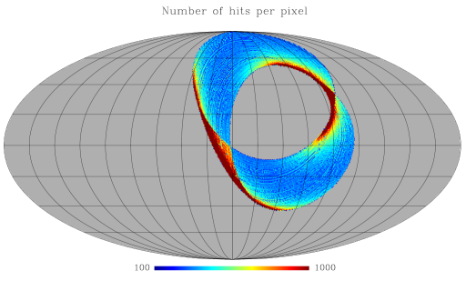
Figure 3: Total number of detector samples per pixels with the 6 bolometers at 353GHz. The map is centered on the Galactic anti–center and grid coordinates are spaced by $20^{\circ}$. The Galactic plane is scanned from about 85 to 120 and 180 to $200^{\circ}$. The covered fraction of the sky is 17 %.

4.4 Absolute Calibration

For absolute calibration we use the so-called FIRAS “Dust spectrum Maps” data, which are spectral sky maps (from 100 $\mu$m to 4 mm for each $7^{\circ}$ pixel) from which the CMB, interplanetary dust and interstellar line emission have been subtracted. Each FIRAS spectrum is fitted with a modified blackbody emission law: $S=\tau(\nu/\nu_{0})^{\beta}P(\nu,T_{dust})$, where $\beta$ is an empirical spectral index. This model is then convolved with the Archeops bandpass filter. The Archeops data are smoothed to match FIRAS beam. The calibration is then obtained from a correlation between FIRAS and Archeops Galactic latitude profiles, and has an absolute accuracy of about 6%. This affects only the absolute values of $I,\;Q,\;U$ and neither the degree of polarization nor its orientation. A detailed description of the calibration is given in (Lagache (2003); Benoît et al. 2003c ). In order not to include polarization effects in this calibration, we calibrated the total intensity of each pair of cross–calibrated bolometers against FIRAS. All numerical values throughout the paper are given in $\mathrm{mK_{RJ}}$. A brightness of $1\;\mathrm{mK_{RJ}}$ is equivalent to $4.36\;\mathrm{MJy.sr}^{-1}$ using IRAS convention (constant $\nu I_{\nu}$) for Archeops 353 GHz bandpass filter, and 15.4 $\mathrm{mK_{CMB}}$.

4.5 Inversion method

For a given direction of observation ${\bf n}$, the associated usual coordinate vectors $({\bf e_{\varphi}},-{\bf e_{\theta}})$ tangential to the sphere are chosen as the reference frame to express Stokes parameters $(I,Q,U)$. The sign accounts of Galactic longitudes and latitudes on the sphere that are clockwise oriented. Let ${\bf E}$ be the incident electric field, $E$ its amplitude and $\psi$ its angle with respect to ${\bf e_{\varphi}}$ in the tangential plane, defined in the range $[0^{\circ},180^{\circ}]$, then

$$Q \equiv |{\bf E}\cdot{\bf e_{\varphi}}|^{2}-|{\bf E}\cdot{\bf e_{\theta}}|^{2}$$ (2)

$$U \equiv |{\bf E}\cdot{\bf e_{\varphi}^{45}}|^{2}-|{\bf E}\cdot{\bf e_{\theta}^{45}}|^{2},$$ (3)

where the superscript 45 means that the original coordinate vectors have been rotated clockwise by 45 degrees.

In this subsection, the polarizers are assumed to be calibrated against an unpolarized source (cf. subsec. 4.3,  4.4). The calibrated polarimeter at an angle $\alpha$ with respect to ${\bf e_{\varphi}}$ measures

$$m(\alpha) = c\;E^{2}\cos^{2}(\alpha-\psi)+n$$ (4)

$$= c\;(I+Q\cos 2\alpha+U\sin 2\alpha)+n,$$

where the noise $n$ depends on time, $\alpha$ depends on the bolometer and on the pixel, and $c$ is the bolometer calibration coefficient. In order to make a $n_{pix}$ map, all samples must be taken into account to include noise correlations (in time and from pixel to pixel) and equation (4) is generalized to :

$${\bf M}=\mathcal{A}{\bf S}+{\bf N},$$ (5)

where M is the time ordered vector of the $n_{t}\times n_{bol}$ measures, S the $(3\leavevmode\nobreak\ n_{pix})$–vector Stokes map of the sky, $\mathcal{A}$ the pointing matrix encoding the pointing information and polarizer angles and N the $n_{t}\times n_{bol}$ noise vector. The $\chi^{2}$ is given by

$$\chi^{2}=(\bf{M}-\mathcal{A}{\bf S})^{T}\mathcal{N}^{-1}({\bf M}-\mathcal{A}{\bf S})$$ (6)

and is minimized by the solution

$${\bf S}=(\mathcal{A}^{T}\mathcal{N}^{-1}\mathcal{A})^{-1}\mathcal{A}^{T}\mathcal{N}^{-1}{\bf M}.$$ (7)

The covariance matrix is then

$${\bf\Sigma}=(\mathcal{A}^{T}\mathcal{N}^{-1}\mathcal{A})^{-1}.$$ (8)

Solving the linear system (7) is one of the recurrent problems in CMB studies since the matrices and vectors are usually large. In our case, however, the size of the polarized regions correspond to temporal frequencies where the noise is essentially white (in–scan induced noise), and the level of striping in $Q$ and $U$ (cross–scan induced noise) is negligible and therefore we can use the following simplification. When the noise is not correlated from one measurement to another, $\mathcal{N}$ is diagonal and the inversion of large matrices can be avoided. We therefore consider each pixel individually, compute the (3,3)-matrix $\mathcal{A}^{T}\mathcal{N}^{-1}\mathcal{A}$ and the (3)-vector $\mathcal{A}^{T}\mathcal{N}^{-1}{\bf M}$. The system of equations thus involves small mathematical objects and the inversion time is small.

5 Results

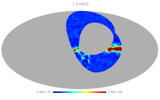
Figure 4: Archeops $I$ map at 353 GHz in $\mathrm{mK}_{RJ}$ smoothed with a 1 degree Gaussian beam.

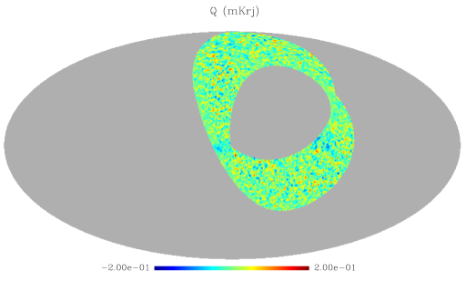
Figure 5: Archeops $Q$ map at 353 GHz in $\mathrm{mK}_{RJ}$ smoothed with a 1 degree Gaussian beam.

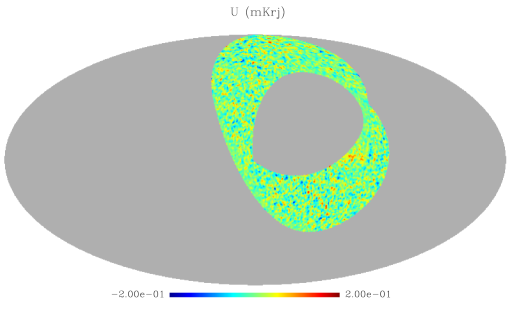
Figure 6: Archeops $U$ map at 353 GHz in $\mathrm{mK}_{RJ}$ smoothed with a 1 degree Gaussian beam.

Once the data are cleaned (Sect. 4.1), they are filtered (Sect. 4.2), calibrated (Sect. 4.4) and combined according to Eq. (5) and inverted with Eq. (7) to produce maps of $I$, $Q$, and $U$. We choose a pixel size of 27.5 arcmin, corresponding to HEALpix (Gorski et al. 1998 ) resolution parameter $n_{\mathrm{side}}=128$. Pixels that have less than 100 detector samples, which correspond to 0.11 sec mission integration time and a $1\,\sigma$ $I$ noise level of $143\leavevmode\nobreak\ \mu\mathrm{K_{RJ}}$ are blanked. For display purposes the maps are smoothed with a 1 deg beam, and these maps are shown in Figs. 4 5 6). The noise estimate for $I,Q,U$ is obtained through Eq. 8.

The dispersion of $Q$ and $U$ at high Galactic latitudes is found to be $\simeq 1.1$ times larger than their noise estimates from the inversion method. This is due to the fact that the noise is not perfectly white. In the analysis that follows we use the measured dispersion as a measure of the noise and not the lower noise estimated from the inversion method. The instantaneous mission $I$ sensitivity is found to be about 48 $\mu\mathrm{K_{RJ}.sec}^{1/2}$. On average, the 1 $\sigma$ noise per pixel of 27 arcmin ($n_{\mathrm{side}}=128$) is found to be 82 $\mu\mathrm{K_{RJ}}$ in intensity and 105 $\mu\mathrm{K_{RJ}}$ in $Q$ and $U$. A statistically significant polarization signal is detected in various locations on the galactic plane. Fig. 7 shows a map of the “normalized squared polarized intensity” defined as the squared polarized intensity $(Q^{2}+U^{2})$ normalized to its variance $(\sigma_{Q}^{2}+\sigma_{U}^{2})$. Twice this quantity behaves has a $\chi^{2}$ probability distribution function with 2 degrees of freedom. A statistically significant signal appears in regions where the normalized squared polarized intensity significantly exceeds a value of unity and several such regions are detected along the galactic plane. We now discuss the results on isolated regions and diffuse medium.

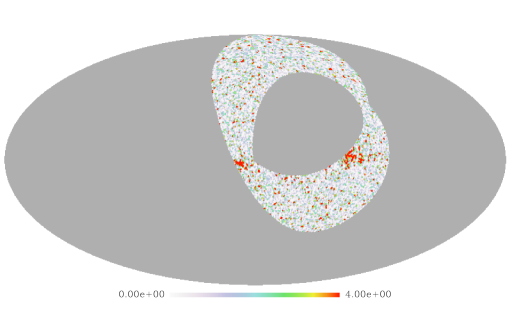
Figure 7: Map of the normalized squared polarized intensity $(Q^{2}+U^{2})/(\sigma_{Q}^{2}+\sigma_{U}^{2})$. Twice this quantity is statistically distributed like a $\chi^{2}$ with 2 degrees of freedom. The 68, 95.4, 99.7% CL of the mapped quantity correspond to 1.1, 3.1, 5.8 respectively.

5.1 Galactic dense clouds

Here we focus on connected regions in which the normalized polarized intensity exceeds the $2\sigma$ level on Fig. 7. The Stokes parameters for these clouds are determined by averaging the pixel values of the unsmoothed maps with weights that are inversely proportional to the variance in the pixels. Table 1 gives the values of $I$, $Q$, $U$, $p$ and $\theta$ for these regions. Because the Taurus cloud region has been well studied by various instruments we give its values separately to facilitate an easy comparison. Since $p$ is not a Gaussian variable, we estimate and correct for the bias on its determination using Monte Carlo simulations. Error bars on $p$ and $\theta$ at 68 % CL are also determined using simulations. The simulations include the cross-calibration errors discussed in Section 4.3.

Cloud index	$I\;(\mathrm{mK_{RJ}})$ (stat) (syst)	$Q\;(\mathrm{mK_{RJ}})$ (stat) (syst)	$U\;(\mathrm{mK_{RJ}})$ (stat) (syst)
0	$1.018\pm 0.015\pm 0.085$	$-0.057\pm 0.021\pm 0.001$	$0.111\pm 0.017\pm 0.008$
1	$0.562\pm 0.014\pm 0.090$	$-0.115\pm 0.019\pm 0.001$	$0.052\pm 0.016\pm 0.003$
2	$1.498\pm 0.011\pm 0.105$	$-0.004\pm 0.014\pm 0.007$	$0.113\pm 0.013\pm 0.014$
3	$0.419\pm 0.021\pm 0.111$	$0.100\pm 0.028\pm 0.013$	$-0.018\pm 0.027\pm 0.009$
4	$0.994\pm 0.023\pm 0.075$	$-0.125\pm 0.029\pm 0.015$	$0.015\pm 0.029\pm 0.010$
5	$0.820\pm 0.011\pm 0.113$	$-0.135\pm 0.014\pm 0.010$	$0.005\pm 0.015\pm 0.005$
6	$0.698\pm 0.004\pm 0.055$	$-0.059\pm 0.005\pm 0.013$	$0.011\pm 0.006\pm 0.004$
7	$0.409\pm 0.010\pm 0.039$	$-0.023\pm 0.014\pm 0.002$	$-0.010\pm 0.013\pm 0.005$
8	$0.271\pm 0.006\pm 0.065$	$-0.001\pm 0.009\pm 0.002$	$-0.021\pm 0.008\pm 0.006$
9	$0.473\pm 0.009\pm 0.080$	$0.001\pm 0.013\pm 0.003$	$0.001\pm 0.011\pm 0.008$

Cloud index	$l$	$b$	Size ($\mathrm{deg}^{2}$)	$p\;(\%)$ (stat) (syst)	$\theta\;(^{\circ})$ (stat) (syst)
0	103.0	1.8	5.9	$12.1^{+1.8}_{-1.8}\pm 1.8$	$59\pm 4.7\pm 1.0$
1	105.8	0.6	7.3	$22.2^{+3.4}_{-3.3}\pm 4.0$	$78\pm 3.7\pm 0.8$
2	109.7	2.1	8.8	$7.5^{+0.9}_{-0.9}\pm 1.5$	$46\pm 3.6\pm 2.0$
3	113.2	-2.7	2.9	$23.3^{+6.5}_{-6.7}\pm 9.7$	$175\pm 7.5\pm 3.2$
4	113.6	-1.2	2.3	$12.3^{+2.8}_{-2.9}\pm 2.6$	$87\pm 6.7\pm 2.8$
5	115.0	2.4	5.9	$16.3^{+1.7}_{-1.7}\pm 3.5$	$89\pm 3.2\pm 1.1$
6	193.0	0.0	21.6	$8.5^{+0.7}_{-0.7}\pm 2.6$	$85\pm 2.8\pm 3.1$
7	159.3	-20.1	18.5	$5.3^{+3.1}_{-3.1}\pm 1.5$	$101\pm 13.6\pm 6.3$
8	165.6	-9.0	50.1	$7.2^{+2.8}_{-2.8}\pm 4.1$	$133\pm 11.5\pm 3.8$
9	174.4	-13.6	21.0	$<3.4$	$23\pm 16.0\pm 104.7$

Table 1: Top: Stokes parameters of significantly polarized Galactic clouds (above double line) and of Taurus complex (below double line). Bottom: Coordinates of the maximum of intensity, measured area, degree and orientation of polarization of these clouds. Systematic error bars are derived from the dispersion of the results with different filtering parameters on the timelines (see Sect. 6.4). Last line correspond to a 95 % CL upper limit. Angles are counted clockwise, 0 being parallel to the Galactic plane. A brightness of $1\;\mathrm{mK_{RJ}}$ is equivalent to $4.36\;\mathrm{MJy.sr}^{-1}$ using IRAS convention (constant $\nu I_{\nu}$) for Archeops 353 GHz bandpass filter. Absolute calibration error of 6 % is not included.

5.2 Diffuse Galactic regions

In this section we determine whether there is a coherent level of polarization on large regions without defining any cloud boundaries. For that purpose and to enhance the signal to noise ratio, we divide the Galaxy into 5 deg wide bands along Galactic longitude. For each band we construct three latitude profiles consisting of the values of $I$, $Q$ and $U$ as a function of latitude; we use binning of 2 degrees in latitude. These three profiles are then used to find a unique polarization vector $(p,\theta)$ characterizing the region corresponding to the profile. We avoid the bias in the determination of the polarization vector using simulations. An example of a profile is shown in Fig. 8, and the results are summarized in Table 2 and in Fig. 9. Coherent polarization levels of few percents are significantly detected up to 5 % at the 3 to 4 $\sigma$ level for several longitude bands, some of which include the clouds already discussed in the previous section. Even after masking these clouds, a significant coherent polarization remains in the same longitude bands.

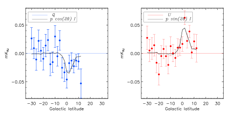
Figure 8: Scaling of $I,\;Q,\;U$ Galactic latitude profiles e. g.  for a Galactic longitude range $[105,110]^{\circ}$. The profiles enable to constrain diffuse polarization.

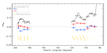
Figure 9: Summary figure of diffuse Galactic polarization. The intensity (divided by 10) is represented in black and is taken to be the average value for $-2\leq b\leq 2$ in each longitude band. The thin solid line is the same value in $2^{\circ}$ wide bands. The direction of polarization for every bin is represented below in green, and the length of the dash is proportionnal to the degree of polarization $p$ in %. The horizontal error bars represent the width of the longitude bins, which is $5^{\circ}$ except for the edge bins. Values are summarized in Tab. 2.

Gal. Long. Range $(^{\circ})$	$I\;(\mathrm{mK_{RJ}})$ (stat) (syst)	$Q\;(\mathrm{mK_{RJ}})$ (stat) (syst)	$U\;(\mathrm{mK_{RJ}})$ (stat) (syst)
$85\;\;90$	$1.34\pm 0.093\pm 0.040$	$0.008\pm 0.009\pm 0.000$	$0.001\pm 0.008\pm 0.004$
$90\;\;95$	$1.47\pm 0.088\pm 0.053$	$0.012\pm 0.008\pm 0.002$	$0.010\pm 0.007\pm 0.002$
$95\;\;100$	$1.12\pm 0.085\pm 0.052$	$-0.001\pm 0.008\pm 0.000$	$-0.019\pm 0.007\pm 0.003$
$100\;\;105$	$0.79\pm 0.081\pm 0.062$	$-0.030\pm 0.008\pm 0.001$	$0.037\pm 0.006\pm 0.005$
$105\;\;110$	$1.03\pm 0.076\pm 0.062$	$-0.030\pm 0.007\pm 0.003$	$0.038\pm 0.006\pm 0.001$
$110\;\;115$	$1.21\pm 0.071\pm 0.031$	$-0.033\pm 0.007\pm 0.000$	$0.042\pm 0.007\pm 0.002$
$115\;\;120$	$0.62\pm 0.069\pm 0.029$	$-0.009\pm 0.008\pm 0.009$	$0.030\pm 0.009\pm 0.006$
$180\;\;185$	$0.52\pm 0.068\pm 0.048$	$-0.027\pm 0.008\pm 0.011$	$-0.007\pm 0.008\pm 0.000$
$185\;\;190$	$0.59\pm 0.061\pm 0.055$	$-0.028\pm 0.006\pm 0.008$	$0.002\pm 0.007\pm 0.004$
$190\;\;195$	$0.82\pm 0.041\pm 0.055$	$-0.044\pm 0.005\pm 0.011$	$0.010\pm 0.006\pm 0.001$
$195\;\;197$	$0.43\pm 0.029\pm 0.042$	$-0.011\pm 0.008\pm 0.005$	$0.013\pm 0.009\pm 0.003$

Gal. Long. Range $(^{\circ})$	$p\;(\%)$ (stat) (syst)	$\theta\;(^{\circ})$ (stat) (syst)
$85\;\;90$	$0.2^{+0.6}_{-0.5}\pm 0.1$	$4\pm 34\pm 15$
$90\;\;95$	$0.9^{+0.5}_{-0.5}\pm 0.3$	$20\pm 16\pm 6$
$95\;\;100$	$1.6^{+0.7}_{-0.6}\pm 0.4$	$134\pm 15\pm 0$
$100\;\;105$	$6.0^{+0.9}_{-0.8}\pm 1.0$	$65\pm 4\pm 2$
$105\;\;110$	$4.7^{+0.6}_{-0.7}\pm 0.6$	$64\pm 4\pm 1$
$110\;\;115$	$4.3^{+0.5}_{-0.6}\pm 0.2$	$64\pm 4\pm 0$
$115\;\;120$	$4.8^{+1.3}_{-1.5}\pm 1.6$	$54\pm 8\pm 9$
$180\;\;185$	$5.2^{+1.6}_{-1.4}\pm 2.6$	$98\pm 9\pm 3$
$185\;\;190$	$4.6^{+1.0}_{-1.0}\pm 1.9$	$88\pm 8\pm 4$
$190\;\;195$	$5.4^{+0.6}_{-0.6}\pm 1.7$	$84\pm 4\pm 1$
$195\;\;197$	$3.5^{+1.9}_{-2.1}\pm 1.6$	$65\pm 17\pm 8$

Table 2: Top: Stokes parameters of $5^{\circ}$ Galactic longitude bands. The intensity is the average over the longitude band and $b$ taken in the range $[-2^{\circ},2^{\circ}]$. $Q$ and $U$ are scaled from that intensity using the latitude profile fit. Bottom: Degree and orientation of polarization for these bands. Angles are counted clockwise, 0 being parallel to the Galactic plane. Due to incomplete sky coverage some longitude bands are not quoted. Systematic error bars are derived from the dispersion of the results with different filtering parameters on the timelines (Sect. 6.4).

6 Systematics and cross–checks

It is the first time that a significant detection of polarization from the diffuse submillimetre Galactic dust emission is reported. Before giving interpretation, we discuss the levels of possible systematics that can alter the results.

6.1 Cross checking different methods of polarization determination

To test our $Q$ and $U$ results, we have employed two additional techniques to derive their values. Instead of finding a combined solution for $I$, $Q$, and $U$ using equation (7) we determined $(Q,U)$ from differences of cross–calibrated pair of bolometers by differencing the time-ordered data. Following equation (4) one can write

$$\Delta m(\alpha) \equiv m(\alpha)/c-m(\alpha+\pi/2)/c^{\prime}$$ (9)

$$= 2\;(Q\cos 2\alpha+U\sin 2\alpha)+n^{\prime}.$$

where $c$ and $c^{\prime}$ are the calibration constants of the bolometers (see Eq. 4). In this method the information on the total intensity $I$ is lost. However, the noise power spectrum of the difference $\Delta m$ is much flatter at low frequencies than for individual bolometers because the differencing scheme removes common spurious unpolarized signals such as the atmosphere or common gain drifts.

We apply the map making algorithm outlined in eqs. (5, 7) to the difference $\Delta m$ and re–derive $Q$ and $U$ values. The results are consistent within one $\sigma$ with the results reported in Tables 1 and 2 for all clouds and galactic profiles.

In the second technique we simply bin the difference of the TOD of a given cloud in $10^{\circ}$ bins of the polarizer angle $\alpha$. The binned signal is fit with a function of the form of Eq. (9) to obtain $Q$ and $U$ values. This method does not depend on the map making algorithm which was used both as the main analysis technique and for the alternate method described earlier in this Section. The results of the binning for the Gemini cloud (centered on $(l,b)=(194.5,-0.9)$) are shown in Fig. 10, but have been carried out for all the clouds for which Table 1 gives results. For the Gemini cloud the fit has a $\chi^{2}/ndf$ of 0.93 and gives $Q=-0.056\pm 0.006\leavevmode\nobreak\ \mathrm{mK_{RJ}}$ , $U=0.020\pm 0.006\leavevmode\nobreak\ \mathrm{mK_{RJ}}$ and $\theta=80.2\pm 3.4$ deg. The results show that Eq. (9) is a good fit to the binned data and that the $Q$ and $U$ values are in good agreement with polarization values deduced from the other two techniques described earlier. Figure 10 also shows consistency between the two sets of three photometers (each with two orthogonal bolometers) and between the data taken at two different times during the flight.

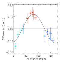
Figure 10: Fit of difference–timelines (filtered differences of bolometer outputs of the same pair) as a function of their associated polarizer angle for the Gemini cloud (cloud index 6 in Table 1). This cloud is observed at two different time intervals and provides useful consistency check, independent of the inversion method. Values are averaged in $10^{\circ}$ angle bins. Different symbols and colors are for the different pairs Red squares, light blue circles and blue triangles are for the first, second and third pair resp. Empty symbols refer to the first time interval, filled ones refer to the second one. The global fit has a $\chi^{2}/ndf$ of 0.93 and gives: $Q=-0.056\pm 0.006\leavevmode\nobreak\ \mathrm{mK_{RJ}}$, $U=0.020\pm 0.006\leavevmode\nobreak\ \mathrm{mK_{RJ}}$ and $\theta=80.2\pm 3.4$ deg, in good agreement with values deduced from the maps and mentioned in Tab. 1.

6.2 Consistency between bolometers

Figure 11: $Q$ (left), $U$ (right) determined on the Gemini cloud ($l\simeq 193^{\circ},\leavevmode\nobreak\ b\simeq-1.2^{\circ}$) with sets of two pairs of 353 GHz bolometers out of the three available. Each point is labeled with the pairs used to compute it. The solid line is the value determined on the map using the three pairs, the dashed lines are the 1 $\sigma$ errors on this value.

In order to check the consistency between the three pairs of bolometers, we computed $Q$ and $U$ with various combinations of only two pairs out of the three available. Figure 11 shows that all the results are in good agreement and are consistent with the values derived using all three pairs. Moreover, the photometric accuracy of the $I$ map can be checked against SFD template at 353 GHz. We find a consistency within 10 %.

6.3 Uncertainties on cross–calibration

The validity of the cross-calibration procedure depends critically on the assumption that the regions over which signals from different detectors are compared are on average not polarized. This assumption can fail in various ways and here we test for these failures.

If one region which is highly polarized biases the cross-calibration coefficients, then the polarization derived in other locations in the galaxy should be correlated with intensity. Visual inspection of the maps does not reveal an obvious correlation. For example, the right part of the intensity map (near Cygnus), which is the brightest (Fig. 4), has no polarization counterpart.

A large scale coherent polarization can induce a systematic error in the cross-calibration if the polarizers crossed the Galaxy at constant angles. Because of our scan pattern the polarizers rotate as they cross the galaxy. To understand the effect quantitatively we carried out simulations where the entire galaxy (Schlegel et al. (1998)) was polarized at the 5% level with constant orientation. The reconstructed cross–calibration coefficients, derived using the assumption that the galaxy does not have a large scale coherent polarization, were biased at the 2-3% level and modified the polarization at the level $\Delta p\sim 1\leavevmode\nobreak\ \%$.

The galaxy is most probably not polarized at a constant level and orientation. We derive the cross-calibration errors by simulating several test maps of the Galaxy using SFD templates with a 5% polarization with random orientations in various regions. We perform a first iteration of the cross calibration assuming that these simulated galaxy maps are not polarized, and we then reconstruct the polarization map using the derived cross-calibration coefficients. We perform a second cross-calibration after masking the regions that were found to be polarized after the first iteration with a significance level of larger than 2 $\sigma$. The $1\sigma$ uncertainty in the extraction of the cross calibration coefficients after this second iteration was 2%. The $1\sigma$ uncertainty in the determination of the Stokes parameters in the regions that had 5% polarization was less than 1% in $I$, and about 3–5 % in $Q$ and $U$, depending on the intensity of the chosen polarized region.

We can also check the cross–calibration process on the three intensity maps that can be deduced from the three pairs of bolometers. The histograms shown on Fig. 12 give the intensity difference between two pairs normalized by the expected noise. The histograms are Gaussian with a standard deviation of 1 and without any outlyers.

Figure 12: Histograms of the noise normalized difference between the intensity from two pairs of bolometers on the Galaxy ($b\in[-10,10]$). These histograms are compatible with a normal distribution, which shows a good relative calibration reconstruction.

In order to test the reconstruction of the noise characteristics, we also perform a null test with the data themselves by randomizing the angle of each polarizer pair at each sample before applying the inversion (7). As maps are computed with rather large pixels ($n_{side}=128$), this effectively cancels out any diffuse sky polarized signal as checked on simulations while conserving the noise properties. If one considers the values of $Q$ and $U$ derived from these “randomized” maps for the ten clouds of Table 1, one can form the $\chi^{2}/ndf$ of the hypothesis that they all be zero. We find a compatibility at the 90% CL.

6.4 Filtering effects

Using the above mentioned simulations (Schlegel et al. (1998)), we observe that time domain filtering removes the large scale diffuse emission (which broadly has a cosecant law behaviour). It represents usually 10–20 %, sometimes 30 % of the total intensity along the line of sight. By changing the filtering parameters on the real data timelines (e.g. the mask, the frequency cut), we observe a similar effect, principally on $I$ and much less on $Q$ and $U$. We derive the systematic error bars (Tabs. 1 and 2) from the dispersion of the results obtained with these different filterings. The polarized emission characterized by $Q$ and $U$ and its orientation are therefore more accurately determined than the degree of polarization.

6.5 Beam effects and time constants

Beams are found to be nearly identical between the two bolometers of a same pair. Nevertheless, slight beam mismatch convolved with the Galactic gradient could generate a spurious polarization signal. This effect has been estimated to be of at most 10 $\mu K$, below our statistical uncertainties. This is also true for uncertainties on time constants which are less than 2 millisec (i.e. 6 arcmin). The cross–calibration found using Jupiter agrees with the cross-calibration using the Galactic profiles to better than $1.5\;\sigma$ uncertainty for each bolometer.

7 Interpretation of the results

The emission of two cloud complexes appear to be strongly polarized at 353 GHz. One large complex is in Cassiopeia (clouds 1–5 in Tab. 1) with an area of $33\leavevmode\nobreak\ \mathrm{deg}^{2}$. This area includes the supernova remnant CasA, although the center is detected in the processing as a point source and is not projected. The other complex coincides with the southern part of Gem OB1 (cloud 6 in Tab. 1). Interestingly, the observed part of the Cygnus complex is not fount to be significantly polarized.

The orientation of the polarization that we find using the galactic profiles is found to be coherent on large scales and is also consistent with that found in clouds. Overall, the orientation is nearly orthogonal to the Galactic plane. It was long noted from optical polarization studies that neighbouring stars had similar polarization directions, with a degree of polarization $p_{V}$ more or less proportional to reddening giving an empirical relation : $p_{V}=0.03A_{V}$ (Whittet (1996); Goodman (1996)). The basic explanation is that a large scale Galactic magnetic field induces alignment of elongated ISD grains. Starlight polarization measures the projection of the direction of polarization on the plane of the sky. However, optical polarization measurements sample only rather low reddening lines of sight and near infrared polarimetric studies yield ambiguous results concerning denser clouds (Whittet (1996); Goodman (1996)). On the other hand, submm polarization is free from opacity effects and samples all the ISD material along the line of sight. The 353 GHz band is nearly on the Rayleigh–Jeans side of dust thermal emission, so grains of various temperatures should not have very different contributions in different radiation fields. If the grains that produce visible extinction are responsible for submm emission with the same efficiency, then an average polarization of at least 3 % (Stein (1966)) is expected at 353 GHz. As shown in Tab. 2, we find a level slightly above this figure and much higher in some clouds therefore indicating a very efficient grain alignment mechanism (Hildebrand & Dragovan (1995)). Moreover, starlight extinction polarization measurements are predicted to be orthogonal to the polarized thermal emission. Catalogs of starlight polarization have been gathered (Fosalba et al. (2002) and references therein) and show a global orientation parallel to the Galactic plane in this longitude range, compatible within 20 to $30^{\circ}$ with the orientation of diffuse medium emission as shown in Tab. 2 and Fig. 9. If the magnetic field follows the spiral arms, one can also expect, as we measure only its projection onto the plane of the sky, that some longitudes should have a reduced apparent polarization (see Fig. 5 in Fosalba et al. (2002)). The very low polarization found on Cygnus is in qualitative agreement with this prediction as the spiral arm lies along the line of sight in this longitude range.

A coherence of the orientation of polarization between the diffuse medium and denser clouds is generally observed, except for the cloud G113.2-2.7. It seems that the global magnetic field that pervades the Galactic plane also goes deeply into some denser clouds and is not tangled by turbulence effects. However, the degree of polarization may vary by as much as a factor two inside the same cloud complex. This probably comes from the local variability of the magnetic field.

The present observations are complementary to the far infrared and millimetre polarimetry as reviewed by (Hildebrand (1996)) because here we probe much more diffuse lines of sight.

Although the instrument sensitivity does not allow to measure directly high Galactic latitude dust polarization, we can extrapolate our results to these regions, assuming that the coherence of the magnetic field and the properties of the ISD are similar to the ones in the Galactic plane. It can then be anticipated that dust polarized emission will be the major foreground to CMB polarization studies at the level of 10 % of its intensity, as anticipated by (Prunet et al. (1998)). The integration along the line of sight of various orientations tends to decrease the overall effect of polarization in the Galactic plane, whereas at high latitude, this depolarization effect should be smaller.

8 Conclusions

Archeops provides the first large coverage maps of Galactic submm emission with 13 arcmin resolution and polarimetric capabilities at 353 GHz. We find that the diffuse emission of the Galactic plane in the observed longitude range is polarized at the 4-5 % level except in the vicinity of the Cygnus region. Its orientation is mostly perpendicular to the Galactic plane and orthogonal, as expected, to the orientation of starlight polarized extinction. Several clouds of few square degrees appear to be polarized at more than 10 %. This suggests a powerful grain alignment mechanism throughout the interstellar medium. Our findings are compatible with models where a strong coherent magnetic field coplanar to the Galactic plane follows the spiral arms, as observed in external Galaxies.