Reconstructing Three-dimensional Structure of Underlying Triaxial Dark Halos From X-ray and Sunyaev–Zel’dovich Effect Observations of Galaxy Clusters

Abstract

While the use of galaxy clusters as tools to probe cosmology is established, their conventional description still relies on the spherical and/or isothermal models that were proposed more than 20 years ago. We present, instead, a deprojection method to extract their intrinsic properties from X-ray and Sunyaev–Zel’dovich effect observations in order to improve our understanding of cluster physics. First we develop a theoretical model for the intra-cluster gas in hydrostatic equilibrium in a triaxial dark matter halo with a constant axis ratio. In this theoretical model, the gas density profiles are expressed in terms of the intrinsic properties of the dark matter halos. Then, we incorporate the projection effect into the gas profiles, and show that the gas surface brightness profiles are expressed in terms of the eccentricities and the orientation angles of the dark halos. For the practical purpose of our theoretical model, we provide several empirical fitting formulae for the gas density and temperature profiles, and also for the surface brightness profiles relevant to X-ray and Sunyaev–Zel’dovich effect observations. Finally, we construct a numerical algorithm to determine the halo eccentricities and orientation angles using our model, and demonstrate that it is possible in principle to reconstruct the 3D structures of the dark halos from the X-ray and/or Sunyaev-Zel’dovich effect cluster data alone without requiring priors such as weak lensing informations and without relying on such restrictive assumptions as the halo axial symmetry about the line-of-sight.

1 INTRODUCTION

Understanding of statistical properties of dark matter halos has been significantly advanced in recent years, largely owing to the development of high-resolution numerical simulations (Navarro, Frenk, & White, 1996, 1997; Fukushige & Makino, 1997; Moore et al., 1998; Jing & Suto, 2000, 2002). Given those theoretical/empirical successes, a next natural question is how to apply them for the description of real galaxy clusters. While there exist a number of attempts along this line, they usually make the unrealistic assumption of the halo spherical symmetry (Makino, Sasaki & Suto, 1998; Suto, Sasaki & Makino, 1998; Yoshikawa & Suto, 1999). This paper describes a methodology to reconstruct the three-dimensional (3D) structure of dark halos from the two-dimensional (2D) surface brightness profiles of intra-cluster gas from the X-ray and/or Sunyaev-Zel’dovich (SZ) effect observations assuming that the halos are triaxial ellipsoids with a constant axis ratio.

Indeed it is a classical problem in astrophysics to determine the 3D properties of astronomical objects from the observed 2D counterparts (e.g., Lucy, 1974; Fabricant et al., 1984; Dehnen & Gerhard, 1993; Binney, Davies, & Illingworth, 1990; Gerhard & Binney, 1996). Deprojecting galaxy clusters is one of the most important applications. Fabricant et al. (1984) analyzed the X-ray surface brightness map of clusters, and showed that their mass distribution is far from being spherical. Zaroubi et al. (1998) developed a general method of deprojecting the 2D images of rich clusters based on the Fourier slice theorem to reconstruct the 3D cluster structures. Later their technique was tested against numerically simulated galaxy clusters (Zaroubi et al., 2001). Yoshikawa & Suto (1999) proposed a deprojection method for spherical clusters based on the Abel integral. Reblinsky (2000) provided a parameter-free Richardson-Lucy algorithm to reconstruct the 3D halo potential, and demonstrated its stability by applying it to gas-dynamical simulations. Dore et al. (2001) provided a perturbative approach to the cluster deprojection, taking into account the non-isothermality and asphericity of galaxy clusters. Recently, Fox & Pen (2002) also considered the problem of deprojecting aspherical clusters. They first constructed a parameterized 3D axisymmetric cluster model, and determined the 3D cluster shapes through the $\chi^{2}$-fitting between the model predictions and the simulated cluster data.

All the previous approaches, however, were based on rather restrictive assumptions such as the cluster axial symmetry (e.g., oblate or prolate) about the line-of-sight, and/or the isothermality of galaxy clusters. Furthermore in their approaches, it was required to combine X-ray and/or SZ effect data with weak lensing (WL) map, which significantly limits the applicability of the previous methods. In fact, it is generally believed that it would be a difficult task to deproject the clusters from the 2D projected X-ray or SZ observables alone without having such restrictive assumptions and priors given the degeneracy of the parameters due to the the projection process itself.

Lee & Suto (2003; hereafter Paper I) suggested that one may understand the properties of the dark matter halos from the intra-cluster gas profiles. Assuming that the intra-cluster gas is in hydrostatic equilibrium in the triaxial dark matter halos, Paper I derived the 3D density and temperature profiles of the intra-cluster gas from the 1st principles using the perturbation theory, and found an analytic relation between the eccentricities of the intra-cluster gas and the underlying dark halo (see eq.[28] in the Paper I). However, the perturbation result of the Paper I is valid only in the asymptotic limit of the low asphericity, and did not include the effect of the projection of the gas profiles on the plane of the sky. Here, we generalize the works of the Paper I to the case of highly aspherical clusters, and attempt to find a general relation between the dark halos and the intra-cluster gas taking into account the parameter-degeneracy caused by the projection. For the practical purpose of our theoretical modeling, we provide a series of empirical fitting formulae for the 2D and 3D gas profiles which can be used as templates in comparing with the observed profiles of clusters, and demonstrate the degree of the feasibility of the halo reconstruction using the template formulae and the simulated surface brightness maps of X-ray and SZ effect.

The organization of this paper is as follows. In §2 we construct a theoretical model for the intra-cluster gas in hydrostatic equilibrium within the gravitational potential of a triaxial dark matter halo with a constant axis ratio, and provide a series of empirical fitting formulae for the 3D gas profiles in a systematic manner. In §3 we consider the projection of the 3D gas profiles onto the plane of the sky, and provide another series of empirical fitting formulae for the 2D surface brightness density profiles. In §4 we describe a numerical algorithm to determine the 3D structures of the dark halos from the observed 2D cluster surface brightness profiles, and test the algorithm against a numerical toy model. Finally we discuss the final results, and draw our conclusions in §5.

2 MODELING INTRA-CLUSTER GAS PROFILES

2.1 Gravitational Potential of Dark Matter Halos

To predict theoretically the X-ray and SZ profiles of galaxy clusters, one first needs a good physical model for the intra-cluster gas. Here we assume that the intra-cluster gas is either isothermal or polytropic, and in hydrostatic equilibrium within the gravitational potential generated by a concentric and coaxial triaxial dark matter halo.

Consider a triaxial dark halo whose iso-density surfaces are given by the following equation:

$$R^{2}\equiv x^{2}+\frac{y^{2}}{1-e_{b}^{2}}+\frac{z^{2}}{1-e_{c}^{2}},$$ (1)

where the Cartesian system of coordinates $(x,y,z)$ is aligned with the halo principal axes, oriented such that the $x$-axis and $z$-axis run along the major and minor principal axes, respectively. The major axis length of the iso-density surface is denoted by $R$, while $e_{b}$ and $e_{c}$ ($e_{b}<e_{c}$) represent the two constant eccentricities of the ellipsoidal dark halos. Equation (1) implies that the density profile of a triaxial dark matter halo should be a function of the major axis length $R$.

We adopt the density profile of a triaxial dark halo proposed by Jing & Suto (2002):

$$\rho(R)=\frac{\delta_{c}\rho_{\rm crit}}{\left(R/R_{0}\right)^{\alpha}\left(1+R/R_{0}\right)^{3-\alpha}},$$ (2)

where $R_{0}$ is the scale length, $\delta_{c}$ is the dimensionless characteristic density contrast with respect to the critical density $\rho_{\rm crit}$ of the universe at the present epoch, and $\alpha$ represents the inner slope of the density profile. Jing & Suto (2002) showed that $\alpha\approx 1$ on the cluster scale and $\alpha\approx 3/2$ on the galaxy scale. For simplicity and definiteness, we focus on the case of $\alpha=1$ throughout this paper.

The gravitational potential due to the ellipsoidal halos described by equation (2) is formally expressed as (Binney & Tremaine, 1987):

$$\Phi({\bf r}) = -\pi G\sqrt{(1-e^{2}_{b})(1-e^{2}_{c})}\int^{\infty}_{0}\frac{[\psi(\infty)-\psi(m)]}{\sqrt{(\tau+1)(\tau+1-e^{2}_{b})(\tau+1-e^{2}_{c})}}d\tau,$$ (3)

$$\psi(m) = 2\int_{0}^{m}\rho(R)RdR,\quad m^{2}=\frac{x^{2}}{\tau+1}+\frac{y^{2}}{\tau+1-e^{2}_{b}}+\frac{z^{2}}{\tau+1-e^{2}_{c}}.$$ (4)

Equations (3) and (4) along with equation (2) allow one to compute the triaxial halo gravitational potential at least numerically. The halo gravitational potential $\Phi({\bf r})$ depends on $\delta_{c}$, $\rho_{\rm crit}$,$R_{0}$ as well as $e_{b}$, $e_{c}$, $\alpha$. However, the dependence of $\Phi({\bf r})$ on $\delta_{c}$, $\rho_{\rm crit}$, and $R_{0}$ can be separated out by introducing a dimensionless potential $\tilde{\Phi}$ that depends only on $e_{b}$, $e_{c}$ and $\alpha$ such that

$$\tilde{\Phi}({\bf r};e_{b},e_{c},\alpha)\equiv\frac{\Phi({\bf r};e_{b},e_{c},\alpha,\delta_{c},\rho_{\rm crit},R_{0})}{4\pi G\delta_{c}\rho_{\rm crit}R^{2}_{0}}.$$ (5)

2.2 Gas Density and Temperature Profiles in terms of Halo Potential

To determine the intra-cluster gas profiles in terms of the halo potential, it is necessary to specify the equation of state for the intra-cluster gas. We consider both the isothermal and the polytropic cases in order.

2.2.1 Isothermal gas

The equation of state for the isothermal gas is given as

$$P_{\rm g}({\bf r})=P_{\rm g0}\frac{\rho_{\rm g}({\bf r})}{\rho_{\rm g0}},$$ (6)

where $P_{\rm g}$ and $\rho_{\rm g}$ represent the gas pressure and the gas density, respectively. In what follows, the subscript $0$ of some physical variable indicates the value of that physical variable at the center ${\bf r}=0$.

The density profile of the isothermal gas in hydrostatic equilibrium is given as

$$\rho_{\rm g}({\bf r})=\rho_{\rm g0}\exp\left[-\kappa\{\tilde{\Phi}({\bf r})-\tilde{\Phi}_{0}\}\right].$$ (7)

We define a dimensionless isothermal gas constant $\kappa$ as

$$\kappa\equiv\frac{4\pi G\mu_{g}m_{p}\delta_{c}\rho_{\rm crit}R^{2}_{0}}{k_{B}T_{\rm g}},$$ (8)

where $m_{p}$ is the proton mass, $\mu_{g}$ is the mean molecular weight of the intra-cluster gas, $k_{B}$ is the Boltzmann constant, and $T_{\rm g}$ is the (constant) gas temperature. Introducing $F_{\Phi}({\bf r})$:

$$F_{\Phi}({\bf r})\equiv\exp\left[-\{\tilde{\Phi}({\bf r})-\tilde{\Phi}_{0}\}\right],$$ (9)

one can rewrite equation (7) as

$$\rho_{\rm g}({\bf r})=\rho_{\rm g0}\,[F_{\Phi}({\bf r})]^{\kappa}.$$ (10)

2.2.2 Polytropic gas

The equation of state for the polytropic gas with the polytropic index of $\gamma$ $(\neq 1)$ is given as

$$P_{\rm g}({\bf r})=P_{\rm g0}\left[\frac{\rho_{\rm g}({\bf r})}{\rho_{\rm g0}}\right]^{\gamma},$$ (11)

and its density and temperature profiles in hydrostatic equilibrium are found as

$$\rho_{\rm g}({\bf r})=\rho_{\rm g0}\left[1-\kappa_{p}\{\tilde{\Phi}({\bf r})-\tilde{\Phi}_{0}\}\right]^{1/(\gamma-1)},\qquad T_{\rm g}=T_{\rm g0}\left[1-\kappa_{p}\{\tilde{\Phi}({\bf r})-\tilde{\Phi}_{0}\}\right].$$ (12)

We define a dimensionless polytropic gas constant $\kappa_{p}$ as

$$\kappa_{p}\equiv\frac{\gamma-1}{\gamma}\frac{4\pi G\mu_{g}m_{p}\delta_{c}\rho_{\rm crit}R^{2}_{0}}{k_{B}T_{\rm g0}},$$ (13)

and introduce $F_{\Phi}({\bf r})$:

$$F_{\Phi}({\bf r})\equiv 1-[\tilde{\Phi}({\bf r})-\tilde{\Phi}_{0}].$$ (14)

Then one can rewrite equation (12) as

$$\rho_{\rm g}({\bf r})=\rho_{\rm g0}\left[1-\kappa_{p}+\kappa_{p}F_{\Phi}({\bf r})\right]^{1/(\gamma-1)},\qquad T_{\rm g}({\bf r})=T_{\rm g0}\left[1-\kappa_{p}+\kappa_{p}F_{\Phi}({\bf r})\right].$$ (15)

2.3 Empirical Fitting Formulae for the Gravitational Potential

We have shown in $\S 2.2$ that the potential function $F_{\Phi}({\bf r})$ defines the density and the temperature profiles of intra-cluster gas completely. In general, $F_{\Phi}({\bf r})$ does not have a closed analytic form when the dark matter halos are triaxial ellipsoids. In Paper I, we computed $F_{\Phi}({\bf r})$ analytically with the perturbation theory assuming $e^{2}_{b}\leq e^{2}_{c}\ll 1$, and related the iso-density surfaces of the intra-cluster gas to those of the dark halos; if the halo iso-density surfaces are triaxial ellipsoids with the eccentricities of $e_{\sigma}$ ($\sigma=b,c$), then the iso-density surfaces of the intra-cluster gas is also well approximated as triaxial ellipsoids with the eccentricities of $\epsilon_{\sigma}$ that are related to $e_{\sigma}$ by

$$\frac{\epsilon^{2}_{\sigma}}{e^{2}_{\sigma}}=\frac{6(1+u)\ln(1+u)+u^{3}-3u^{2}-6u}{2u^{2}[(1+u)\ln(1+u)-u]},$$ (16)

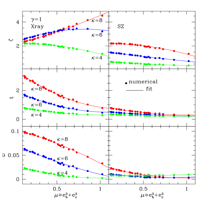
Figure 3: Parameters describing our empirical model of the surface brightness profile (eq.[36]) as a function of $\mu$ for the isothermal case. The filled circles represent the best-fit values to the numerical results at each $\mu$, and the solid curves show the corresponding polynomial fitting curves. Left: X-ray. Right: SZ.

where $u\equiv|{\bf r}|/R_{0}$. Note that the right-hand-side of equation (16) are written in terms of the rescaled spherical radius $u$ instead of the rescaled major axis length, which results from the fact that we neglected the higher-order terms $O(e_{\sigma}^{4})$ in deriving equation (16) with the perturbation theory. Although equation (16) seems complicated, it is a slowly varying function, and well approximated as a constant in the range of $0<u<1$ (see Fig. 3 of Paper I) such that

$$\frac{\epsilon^{2}_{\sigma}}{e^{2}_{\sigma}}\approx 0.7^{2}.$$ (17)

Strictly speaking, equation (17) is valid only in the limit of $e^{2}_{b}\leq e^{2}_{c}\ll 1$ over the range of $0<u<1$. To proceed further in a tractable fashion, however, we extend the validity of equation (17) to $e^{2}_{b}\leq e^{2}_{c}\leq 1$ over the whole range of $u$. In other words, we assume that the iso-density surfaces of the intra-cluster gas are triaxial ellipsoids with the constant eccentricities of $\epsilon_{b},\epsilon_{c}$ that are related to the halo eccentricities $e_{b},e_{c}$ by equation (17). Actually this turns out to be a good approximation as will be shown below.

This assumption allows us to write the potential function $F_{\Phi}({\bf r})$ in terms of the major axis length of the gas iso-density surfaces, $\xi$, defined as

$$\xi^{2}\equiv u^{2}_{x}+\frac{u^{2}_{y}}{1-\epsilon_{b}^{2}}+\frac{u^{2}_{z}}{1-\epsilon_{c}^{2}}=\frac{1}{R_{0}^{2}}\left(x^{2}+\frac{y^{2}}{1-\epsilon_{b}^{2}}+\frac{z^{2}}{1-\epsilon_{c}^{2}}\right).$$ (18)

After some trials and errors, we find that the following empirical formula fits both equations (9) and (14) quite well:

$$F_{\Phi}(\xi)=\left(\frac{1+\eta\xi^{p}}{1+\beta\xi^{p}}\right)^{q},$$ (19)

where $\beta$, $p$, $q$, and $\eta$ are free parameters. The four free parameters are not constant but supposed to be functions of the halo eccentricities. We determine the functional form of each parameter by taking the following steps.

1. Compute $F_{\Phi}({\bf r})$ numerically using equations (3) and (4) for various values of $e_{b}$ and $e_{c}$.

2. Fit those numerical data points to the empirical model (eq. [19]) and obtain the best-fit values of $\beta$, $p$, $q$, and $\eta$ using the Levenberg-Marquardt method (Press et al., 1992).

3. Finally model those best-fit parameters as functions of $e_{b}$ and $e_{c}$. In practice, we find that all the parameters can be written as functions of a single variable $\mu\equiv e^{3}_{b}+e^{3}_{c}$.

We find the following polynomials to provide good fits:

$$\beta = c_{\beta 0}+c_{\beta 1}\mu,$$ (20)

$$p = const.,$$ (21)

$$q = c_{q0}+c_{q1}\mu+c_{q2}\mu^{2},$$ (22)

$$\eta = c_{\eta 0}+c_{\eta 1}\mu.$$ (23)

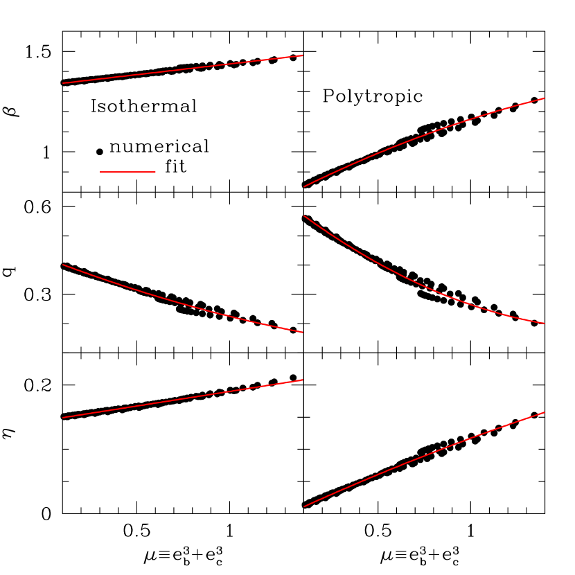
Figure 1: Parameters describing our empirical model of the halo potential profile (eq.[19]) as a function of the halo eccentricities ($\mu\equiv e^{3}_{b}+e^{3}_{c}$). The filled circles represent the best-fit values to the numerical results at each $\mu$, and the solid curves show the corresponding polynomial fitting curves. The intra-cluster gas is assumed to be isothermal (Left) and polytropic (Right).

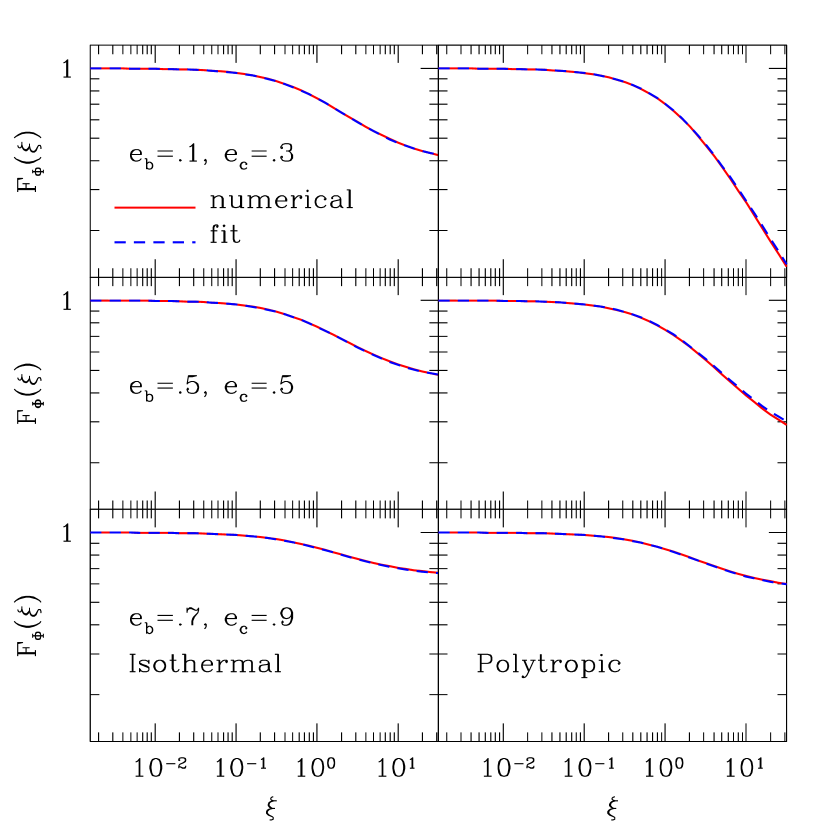
Figure 2: Profiles of gravitational potentials of dark halos. Solid and dashed lines indicate the results of the direct numerical integration and our empirical fitting model, respectively. The intra-cluster gas is assumed to be isothermal (Left) and polytropic (Right). The eccentricities of the underlying dark halos are Top: $e_{b}=0.1$ and $e_{c}=0.3$, Middle: $e_{b}=0.1$ and $e_{c}=0.7$, Bottom: $e_{b}=0.7$ and $e_{c}=0.9$.

Table 1 lists the best-fit values of the polynomial coefficients. The best-fit values of the constant $p$ is determined to be unity for all cases. Figure 1 plots $\beta$, $q$, and $\eta$ as a function of $\mu$. The filled circles indicate the best-fit values of the parameters, while the solid lines represent their polynomial fits. Note that $\eta$ is one order-of-magnitude smaller than $\beta$ for all cases, suggesting that the term associated with $\eta$ can be safely neglected except at the outer part of clusters. The accuracy of the fits is illustrated in Figure 2 where $F_{\Phi}(\xi)$ is plotted against $\xi$. The solid lines represent the numerical results while the dashed lines correspond to equation (19) with the best-fit coefficients of the polynomials plotted in Fig. 1 and listed in Table 1. Our empirical fitting formulae reproduce the numerical results very well for all cases over a wide range of $\xi$ within a fractional error less than $0.5\%$.

The characteristic feature of our fitting model is that all the parameters are expressed in terms of $\mu=e^{3}_{b}+e^{3}_{c}$. Given that the first-order perturbation approach of the Paper I indicated the dependence of the halo potential on $e^{2}_{b}+e^{2}_{c}$, one may have expected the fitting model to depend on $e^{2}_{b}+e^{2}_{c}$ rather than $e^{3}_{b}+e^{3}_{c}$. As a matter of fact, we indeed attempted first to model the parameters in terms of $e^{2}_{b}+e^{2}_{c}$. But, it turned out that the parameter values do not scale in terms of $e^{2}_{b}+e^{2}_{c}$ while they show very good scaling feature in terms of $e^{3}_{b}+e^{3}_{c}$ as shown in Figure 1. We have not yet completely understood the origin of this scaling, but the result is empirically quite robust.

In addition, we note that in the Paper I we derived the gas-halo eccentricity relation (eq. [16]) by using the first-order perturbation theory, and showed that the approximation error can be expressed as a function of $e^{3}_{b}$ and $e^{3}_{c}$ (see eqs [29] and [30] in the Paper I). The dependence of the approximation error on $e^{3}_{b}$ and $e^{3}_{c}$ implies that the higher order terms neglected in the first-order perturbation result may be scaled in terms of $e^{3}_{b}$ and $e^{3}_{c}$. Now that we have used equation (16) to construct the fitting model (eq. [19]), one may expect that equation (19) has similar scaling. In other words, we suspect that the dependence of equation (19) on $e^{3}_{b}+e^{3}_{c}$ rather than $e^{2}_{b}+e^{2}_{c}$ may be related to the scaling of the higher order terms neglected in the first-order perturbation result of the Paper I.

Note also that in our model the gas density/temperature profiles do not approach zero even at large $u$. This feature is ascribed to the hydrostatic equilibrium condition itself. In reality, the hydrostatic equilibrium condition may be satisfied only within some radius, e.g., the virial radius of the cluster. In fact, the halo density profiles at those regions are not well approximated by equation (2) because of the presence of substructures, and so on. This problem, however, is unlikely to limit the validity of our methodology in practice since the X-ray and SZ fluxes from regions beyond the cluster virial radius are usually negligible.

3 PROJECTED SURFACE BRIGHTNESS PROFILES OF INTRA-CLUSTER GAS

Now we are in a position to model the X-ray and SZ surface brightness profiles of triaxial galaxy clusters by incorporating the projection effect into the 3D models developed in $\S 2$. Just for comparison, let us recall that the surface brightness profiles of spherical clusters can be readily evaluated as

$$\Sigma(\theta)=\int_{-\infty}^{\infty}L(\sqrt{d_{\scriptscriptstyle A}^{2}\theta^{2}+z^{2}})dz,$$ (24)

where $\theta$ is the angular radius from the center of the cluster, $d_{\scriptscriptstyle A}$ is the angular diameter distance to the cluster, and $L$ is the emissivity given in terms of $\rho_{g}$ and $T_{g}$ such that $L\propto\rho^{2}_{\rm g}T^{1/2}_{\rm g}$ for bolometric X-ray and $L\propto\rho_{\rm g}T_{\rm g}$ for SZ observations, respectively. For the case of a triaxial cluster, however, the result becomes much more complicated because the 2D projection depends on the relative direction of the line-of-sight of an observer with respect to the principal axes of a triaxial halo. The projection effect of triaxial bodies on the plane of the sky is fully discussed by Stark (1977) and Binney (1985). In what follows we adopt the notation of Binney (1985).

Let $(\theta,\phi)$ be the polar angle of the line-of-sight in the halo principal coordinate system $(x,y,z)$, and let the observer’s coordinate system be defined by Cartesian axes $(x^{\prime},y^{\prime},z^{\prime})$ with $z^{\prime}$-axis aligned with the line-of-sight direction and $x^{\prime}$-axis lying in the $(x,y)$ plane (see Fig. 1 in Oguri, Lee, & Suto, 2003). Then the halo principal coordinate system $(x,y,z)$ is related to the observer’s coordinate system $(x^{\prime},y^{\prime},z^{\prime})$ by

$$x = -\sin\phi x^{\prime}-\cos\phi\cos\theta y^{\prime}+\cos\phi\sin\theta z^{\prime},$$ (25)

$$y = \cos\phi x^{\prime}-\sin\phi\cos\theta y^{\prime}+\sin\phi\sin\theta z^{\prime},$$ (26)

$$z = \sin\theta y^{\prime}+\cos\theta z^{\prime}.$$ (27)

If we use the major axis length $\xi$ defined in equation (18) to characterize the iso-density surfaces, then the projection of $L$ onto the plane of the sky is written as

$$\Sigma(x^{\prime},y^{\prime})\equiv\int^{\infty}_{-\infty}L(\xi^{2})dz^{\prime}=\frac{2}{\sqrt{f}}\int^{\infty}_{0}L(z^{\prime\prime 2}+\lambda^{2})dz^{\prime\prime},$$ (28)

where

$$z^{\prime\prime} = \sqrt{f}\left(z^{\prime}+\frac{g}{2f}\right),$$ (29)

$$\lambda = \frac{1}{\sqrt{f}}(Ax^{\prime 2}+Bx^{\prime}y^{\prime}+Cy^{\prime 2})^{1/2},$$ (30)

$$f = \sin^{2}\theta\left(\cos^{2}\phi+\frac{\sin^{2}\phi}{1-\epsilon_{b}^{2}}\right)+\frac{\cos^{2}\theta}{1-\epsilon_{c}^{2}},$$ (31)

$$g = \sin\theta\sin 2\phi\left(\frac{1}{1-\epsilon_{b}^{2}}-1\right)x^{\prime}+\sin 2\theta\left(\frac{1}{1-\epsilon_{c}^{2}}-\cos^{2}\phi-\frac{\sin^{2}\phi}{1-\epsilon_{b}^{2}}\right)y^{\prime},$$ (32)

$$A = \frac{\cos^{2}\theta}{1-\epsilon_{c}^{2}}\left(\sin^{2}\phi+\frac{\cos^{2}\phi}{1-\epsilon_{b}^{2}}\right)+\frac{\sin^{2}\theta}{1-\epsilon_{b}^{2}},$$ (33)

$$B = \cos\theta\sin 2\phi\left(1-\frac{1}{1-\epsilon_{b}^{2}}\right)\frac{1}{1-\epsilon_{c}^{2}},$$ (34)

$$C = \left(\frac{\sin^{2}\phi}{1-\epsilon_{b}^{2}}+\cos^{2}\phi\right)\frac{1}{1-\epsilon_{c}^{2}}.$$ (35)

Hence $\Sigma(x^{\prime},y^{\prime})=\Sigma(\lambda)$. In other words, the 2D isophotal curves of triaxial galaxy clusters are concentric and coaxial ellipses if their eccentricities $\epsilon_{\sigma}$ of the gas iso-density surfaces are constants. As we noted before, however, it is not exactly the case for our model where the eccentricities $e_{\sigma}$ of the halo iso-density surfaces are constant. Nevertheless this holds approximately (see eq.[17]).

Let us define a dimensionless surface brightness $\tilde{\Sigma}\equiv\Sigma/\Sigma_{0}$ where $\Sigma_{0}\equiv\Sigma(0)$ and $\tilde{\lambda}=\lambda/R_{0}$. In the same spirit as for the 3D model (19), we propose the following empirical model for the 2D surface brightness profiles:

$$\tilde{\Sigma}(\tilde{\lambda};e_{b},e_{c},\kappa,\kappa_{p},\gamma)=\left(\frac{1+\omega\tilde{\lambda}^{s}}{1+\zeta\tilde{\lambda}^{s}}\right)^{t}.$$ (36)

Note that $\tilde{\Sigma}$ depends not only on $\mu$ but also on $\kappa$ (or $\kappa_{p}$), and even on the polytropic index $\gamma$ for the polytropic case. Thus, we consider the isothermal and polytropic cases separately, and obtain the following empirical fits.

For the isothermal gas, the parameters are fitted to the following polynomials of $\mu$ and $\kappa$:

$$\omega = \sum_{i,j=0}^{2}\omega_{ij}\mu^{i}\kappa^{j},$$ (37)

$$\zeta = \sum_{i,j=0}^{2}\zeta_{ij}\mu^{i}\kappa^{j},$$ (38)

$$s = const.,$$ (39)

$$t = \sum_{i,j=0}^{2}t_{ij}\mu^{i}\kappa^{j}.$$ (40)

For the polytropic gas, we fix $\gamma$ to $\gamma=1.15$ following Komatsu & Seljak (2001), and fit the parameters to the following polynomials of $\mu$ and $\kappa$:

$$\omega = \sum_{i,j=0}^{3}\omega_{ij}\mu^{i}\kappa_{p}^{j},$$ (41)

$$\zeta = \sum_{i,j=0}^{3}\zeta_{ij}\mu^{i}\kappa_{p}^{j},$$ (42)

$$s = const.,$$ (43)

$$t = \sum_{i,j=0}^{3}t_{ij}\mu^{i}\kappa_{p}^{j}.$$ (44)

We determine the best-fit values of $\omega_{ij}$, $\zeta_{ij}$, and $t_{ij}$ using the same method as in $\S 2$. First we calculate $\tilde{\Sigma}$ of equation (28) numerically, approximating the integration $\int^{\infty}_{-\infty}Ldz^{\prime}$ to $\int^{z_{c}}_{-z_{c}}Ldz^{\prime}$ where $z_{c}=20R_{0}$ which is roughly twice the virial radius of galaxy clusters (Makino, Sasaki & Suto, 1998). Then we compare the numerical data points of $\tilde{\Sigma}$ with the fitting formula (36), and determine the best-fit values for each point using the Levenberg-Marquardt method. Finally we model the free parameters as polynomials of $\mu$ and $\kappa$ (or $\kappa_{p}$), and determine the best-fit polynomial coefficients.

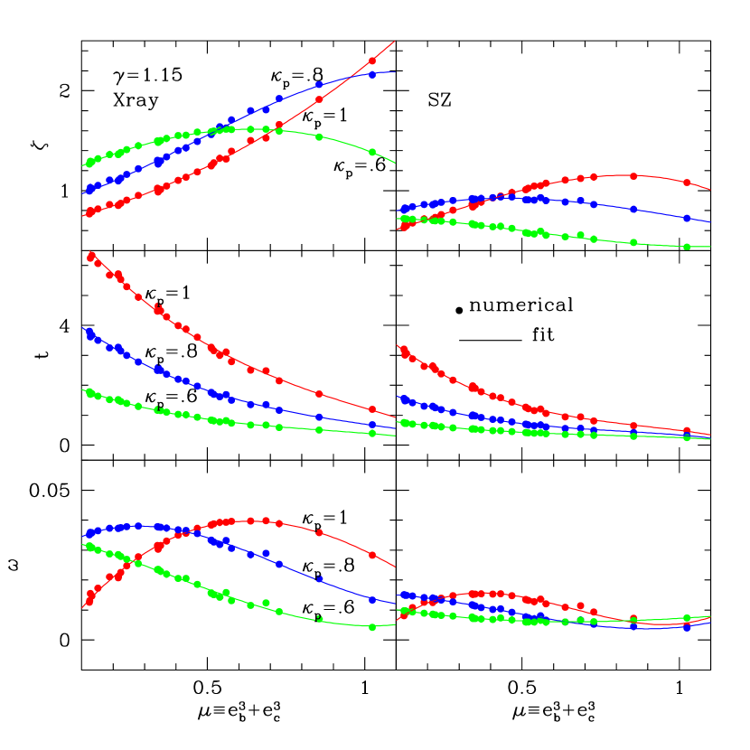
Figure 4: Same as Figure 3 but for the polytropic case.

The best-fit constant values of $s$ is determined to be unity for both the isothermal and polytropic cases just like the 3D model. Figures 3 and 4 plot the best-fit parameters as functions of $\mu$ for three different values of $\kappa$ (or $\kappa_{p}$). It is clear from these figures that the polynomial fitting works quite well for all cases. Tables 2 and 3 list the best-fit coefficients $\zeta_{ij},t_{ij},\omega_{ij}$ for the cases of bolometric X-ray and SZ observations, respectively.

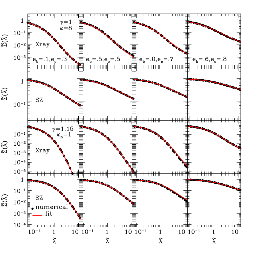
Figure 5: Profiles of the cluster surface brightness. The filled circles are computed numerically, while our fitting models are shown in solid lines. From left to right panels, we adopt the underlying halo eccentricities of $(e_{b},e_{c})=$ (0.1, 0.3), (0.5,0.5), (0.0, 0.7) and (0.6, 0.8). From top to bottom panels, we show the cases of isothermal X-ray ($\kappa=8$), isothermal SZ ($\kappa=8$), polytropic X-ray ($\gamma=1.15$ and $\kappa_{p}=1$), and polytropic SZ ($\gamma=1.15$ and $\kappa_{p}=1$) observations.

Figure 5 illustrates the degree of the accuracy of our fitting formulae. The filled squares represent the numerical results while the solid lines represent our fitting models with the best-fit polynomials of $\zeta$, $t$, and $\omega$. We have found that our fits reproduce the numerical results within the fractional error of $20\%$ for all cases in a range of $0\leq\tilde{\lambda}\leq 10$.

4 DARK HALO RECONSTRUCTION

In the triaxial dark halo model that we adopt here, the halo reconstruction from the X-ray and SZ cluster observations is basically to determine the shapes ($e_{b},e_{c}$) and the orientations ($\theta,\phi$) of the dark halos from the observed surface brightness profiles.

In §3, we construct a parameterized model for the X-ray and SZ surface brightness profiles of galaxy clusters. The model is expressed as a function of the rescaled major axis length of the gas isophotes and characterized by three parameters. It turns out that the rescaled major axis length and the three parameters depend on the eccentricities and the orientation angles of the underlying dark halos, as well as the gas constant. Therefore, we find a way to link the observed 2D surface brightness profiles of galaxy clusters to the 3D structures of the underlying dark halo and the gas constants of the intra-cluster gas as well. In other words, one may expect to determine the values of $(e_{b},e_{c},\theta,\phi)$ and $(\kappa,\kappa_{p})$ by fitting our 2D parameterized models (eqs. [36] – [41]) to the X-ray and SZ cluster data.

To demonstrate how our modeling of cluster profiles can be used in the determination of the shapes and the orientations of dark matter halos, we apply the following reconstruction algorithm to the numerically projected profiles. We first numerically compute $\tilde{\Sigma}$ directly using equations (3)-(28). Then we construct a pixeled map of surface brightness in $N\times N$ grids ($N=32$ in the present example) corresponding to the linear scale of $-10R_{0}\leq x^{\prime},y^{\prime}\leq 10R_{0}$ since $10R_{0}$ is roughly equal to the cluster virial radius (Jing & Suto, 2002). We create several realizations of X-ray and SZ profiles for both isothermal and polytropic cases using various different values of $e_{b},e_{c},\theta,\phi$.

Our reconstruction algorithm proceeds as follows;

• At each pixel point, say, $(x^{\prime}_{i},y^{\prime}_{j})$, build the model $\tilde{\Sigma}^{\rm th}(x^{\prime}_{i},y^{\prime}_{j})$ using equation (36). The model is characterized by five free parameters $e_{b},e_{c},\theta,\phi,\kappa$ (or $\kappa_{p}$) at each point.

• Fit $\tilde{\Sigma}^{\rm th}$ to the observed surface brightness density profiles $\tilde{\Sigma}^{obs}$, and calculate the $\chi^{2}$:

  $$\chi^{2}=\sum_{i,j=1}^{N}\frac{[\tilde{\Sigma}^{\rm th}(x^{\prime}_{i},y^{\prime}_{j})-\tilde{\Sigma}^{obs}(x^{\prime}_{i},y^{\prime}_{j})]^{2}}{\sigma^{2}_{ij}},$$ (45)

  where $\sigma_{ij}$ denotes the observational error at each pixel point $(x^{\prime}_{i},y^{\prime}_{j})$. Those systematic/random errors should depend on specific observation conditions and thus are not easy to estimate a priori. Thus in the following numerical tests, we simply assume that $\sigma_{ij}$ is unity, independent of $i$ and $j$.

• Determine the best-fit values of $e_{b},e_{c},\theta,\phi,\kappa$ (or $\kappa_{p}$) through the $\chi^{2}$ minimization.

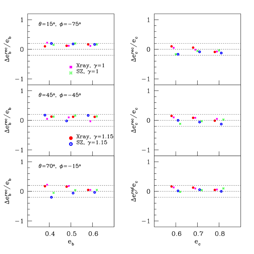
Figure 6: Fractional errors of the reconstructed halo eccentricities. Filled squares, open squares, filled circles, and open circles correspond to the cases of isothermal X-ray, isothermal SZ, polytropic X-ray, and polytropic SZ, respectively. We adopt the orientation angles of the line-of-sight with respect to the cluster in the halo principal frame as $(\theta,\phi)=$ $(15^{o},-75^{o})$, $(45^{o},-45^{o})$, and $(75^{o},-15^{o})$ from top to bottom panels.

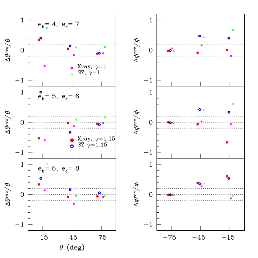
Figure 7: Fractional errors of the reconstructed orientation angles. Filled squares, open squares, filled circles, and open circles correspond to the cases of isothermal X-ray, isothermal SZ, polytropic X-ray, and polytropic SZ, respectively. We adopt the halo eccentricities of $(e_{b},e_{c})=$ = (0.4, 0.7), (0.5, 0.6), and (0.6, 0.8) from top to bottom panels.

The numerical testing results have revealed that the above algorithm works quite well in reconstructing the halo eccentricities within the fractional error of $20\%$ as long as the halo eccentricities are not so small ($e_{b},e_{c}>0.3$), which can be understood considering that our reconstruction algorithm strongly relies on the non-spherical signature, and thus is expected to fail for the case of almost spherical halos with low eccentricities ($e_{b},e_{c}<0.3$). For the low eccentricity cases, the perturbation results of the Paper I may be more useful. Since the low-eccentricity case is not the main interest of the present paper, we do not investigate those cases here. The algorithm also works in reconstructing the orientation angles but suffer relatively large fractional errors. We show the examples of our numerical reconstruction results in Figures 6 and 7 for the following cases of the halo eccentricities and orientation angles: $(e_{b},e_{c})=(0.4,0.7)$, $(0.5,0.6)$, and $(0.6,0.8)$; $(\theta,\phi)=(15,-75)$,$(45,-45)$, $(75,-15)$ in units of degree.

Figure 6 plots the fractional error of the reconstructed eccentricities versus their input values for three different cases of the orientation angles. The left three panels are for $e_{b}$, and the right three panels for $e_{c}$. The top two panels correspond to the case of $\theta=15^{o}$ and $\phi=-75^{o}$, the middle two panels to the case of $\theta=45^{o}$ and $\phi=-45^{o}$, and the bottom three panels to the case of $\theta=75^{o}$ and $\phi=-15^{o}$. For almost all cases, the fractional errors fall within $20\%$.

Figure 7 plots the fractional error of the reconstructed orientation angles versus the original orientation angles for three different cases of the eccentricities. The left three panels are for $\theta$, and the right three panels for $\phi$. The top two panels correspond to the case of $e_{b}=0.4$ and $e_{c}=0.7$, the middle two panels to the case of $e_{b}=0.5$ and $e_{c}=0.6$, and the bottom three panels to the case of $e_{b}=0.6$ and $e_{c}=0.8$. For most cases, the fractional errors fall within $20\%$. However, for a few cases, the fractional errors are larger than $50\%$, indicating that the angle reconstruction is not always stable compared with the eccentricity reconstruction.

5 DISCUSSIONS AND CONCLUSIONS

It was regarded as a difficult task to reconstruct the 3D structures of dark matter halos from the projected 2D surface-brightness maps of X-ray and/or SZ clusters given the parameter-degeneracy caused by the projection process itself. To break the degeneracy, previous approaches had to rely on such restrictive assumptions as the cluster axial symmetry about the line-of-sight and some priors like weak lensing informations. Here we have developed, for the first time, a theoretical framework within which the 3D halo reconstruction is possible in principle without such restrictive assumptions and additional priors.

We derived the density profiles of the intra-cluster gas from the 1st principles, assuming that the intra-cluster gas is either isothermal or polytropic, and in hydrostatic equilibrium within the gravitational potential of concentric and coaxial triaxial dark matter halos. In our theoretical modeling of the intra-cluster gas, the density profiles depend explicitly on the intrinsic properties of the underlying halos (the two halo eccentricities, $e_{b}$ and $e_{c}$). For the case of highly aspherical halos, however, we have found that the gas density profiles cannot be expressed in closed analytic forms. Therefore, we have attempted to find general fitting formulae for the gas density profiles as functions of the halo eccentricities which may be applicable even to highly aspherical clusters. We have found empirically a simple scaling relation with respect to $\mu=e^{3}_{b}+e^{3}_{c}$, and provided a set of fitting formulae for the 3D gas density profiles expressed in terms of $\mu$.

Then, we have incorporated the projection effect into the gas density profiles, and provided another set of fitting formulae for 2D X-ray and/or SZ surface brightness density profiles of galaxy clusters. Unlike the 3D formulae, the 2D formulae are expressed in terms of not only $\mu$ but also the orientation angles of the line-of-sight in the halo principal axes. In other words, we have found a link of the 2D X-ray and/or SZ observables to the shapes and the orientations of the dark matter halos.

We have proposed a numerical algorithm based on our model to determine the halo eccentricities and orientation angles from the observed X-ray and SZ surface brightness density profiles of galaxy clusters. Ideally we have to apply our algorithm to real observation data, but that is beyond the scope of the present paper since it should involve careful treatment of the data image analysis together with various observational systematic effects. Thus we have decided to test the reconstruction algorithm against simple numerical profiles. We found that the algorithm can reconstruct the halo eccentricities fairly accurately if the halo eccentricities are greater than $0.3$. On the other hand, it turns out that the reconstruction of the halo orientation angles are not always accurate, showing large scatters.

Finally, we conclude that our hydrostatic-equilibrium model for intra-cluster gas in triaxial dark halos makes it possible in principle to reconstruct the 3D structures of the dark halos from the X-ray and/or SZ cluster maps, as long as the intra-cluster gas and the dark halos are well approximated to be in hydrostatic equilibrium and the triaxial ellipsoids with a constant axis ratio, respectively. We plan to test our model against real observational data, and hope to report the results elsewhere in the future.

Table 1: Best-fit polynomial coefficients for the profiles of halo gravitational potentials

	Isothermal				Polytropic
($\mu$)	$\beta$	$q$	$\eta$		$\beta$	$q$	$\eta$
0	1.329	0.426	0.146		0.780	0.617	-0.002
1	0.118	-0.246	0.036		0.470	-0.487	0.133
2	-0.010	0.044	0.009		-0.087	0.136	-0.013

Table 2: Best-fit polynomial coefficients for the profiles of the surface brightness in the isothermal case.

	X-ray				SZ
($\mu$  $\kappa$)	$\zeta$	$t$	$\omega$		$\zeta$	$t$	$\omega$
0 0	3.228	-1.127	-0.121		-3.140	0.447	0.014
0 1	-0.206	0.368	0.044		1.133	-0.087	-0.005
0 2	0.008	0.026	-0.002		-0.058	0.018	0.001
1 0	-0.850	3.749	-0.010		3.874	-0.298	0.056
1 1	1.354	-1.314	-0.032		-1.786	0.101	-0.015
1 2	-0.126	0.037	0.003		0.166	-0.027	0.000
2 0	-12.23	-2.184	0.158		0.297	-0.003	-0.042
2 1	2.253	0.840	-0.025		0.342	-0.015	0.014
2 2	-0.082	-0.044	0.000		-0.064	0.011	-0.001

Table 3: Best-fit polynomial coefficients for the profiles of the surface brightness in the polytropic case with $\gamma=1.15$.

	X-ray				SZ
($\mu$  $\kappa_{p}$)	$\zeta$	$t$	$\omega$		$\zeta$	$t$	$\omega$
0 0	2.261	-0.943	-0.257		-3.667	2.542	0.101
0 1	-2.689	0.753	1.027		16.32	-7.786	-0.508
0 2	1.609	6.874	-1.096		-19.30	7.135	0.885
0 3	-0.526	1.328	0.323		7.156	2.345	-0.483
1 0	-0.049	30.48	0.371		-3.390	-19.12	0.424
1 1	13.86	-112.8	-2.301		-0.685	77.61	-1.296
1 2	-27.91	123.3	3.722		19.05	-100.4	0.845
1 3	14.97	-54.25	-1.647		-14.10	32.19	0.145
2 0	-61.22	-67.95	0.836		36.73	34.75	-1.279
2 1	197.2	268.9	-1.902		-125.8	-147.3	4.857
2 2	-199.1	-331.6	0.485		129.1	201.9	-5.537
2 3	63.66	139.9	0.440		-39.35	-79.83	1.742
3 0	56.23	38.90	-0.874		-28.90	-18.29	0.806
3 1	-201.0	-157.9	2.863		107.2	78.73	-3.186
3 2	227.3	202.3	-2.703		-123.9	-110.4	3.918
3 3	-82.35	-86.20	0.743		44.58	46.37	-1.428

References

- Binney (1985) Binney, J. 1985, MNRAS, 212, 767
- Binney & Tremaine (1987) Binney, J., & Tremaine, S. 1987, Galactic Dynamics (Princeton: Princeton Univ. Press)
- Binney, Davies, & Illingworth (1990) Binney, J. J., Davies, R. L., & Illingworth, G. D. 1990, ApJ, 31, 78 Birkinshaw, M. 1999, Phys. Rep., 310, 97
- Dehnen & Gerhard (1993) Dehnen, W., & Gerhard, O. E. 1993, MNRAS, 261, 311
- Dore et al. (2001) Dore, O., Bouchet, F. R., Mellier, Y., & Teyssier, R. 2001, A&A, 375, 14
- Fabricant et al. (1984) Fabricant D., Rybicki, G. & Gorenstein, P. 1984, ApJ, 286, 186
- Fox & Pen (2002) Fox, D. C., & Pen, U. L. 2002, ApJ, 574, 38
- Gerhard & Binney (1996) Gerhard, O., & Binney, J. 1996, MNRAS, 279, 993
- Fukushige & Makino (1997) Fukushiege, T., & Makino, J. 1997, ApJ, 477, L9
- Jing & Suto (2000) Jing, Y. P., & Suto, Y. 2000, ApJ, 529, L69
- Jing & Suto (2002) Jing, Y. P., & Suto, Y. 2002, ApJ, 574, 538
- Komatsu et al. (2001) Komatsu, E. et al. 2001, PASJ, 53, 57
- Komatsu & Seljak (2001) Komatsu, E. & Seljak, U. 2001, MNRAS, 327, 1353
- Lee & Suto (2003) Lee, J. & Suto, Y. 2003, ApJ, 585, 151
- Lucy (1974) Lucy, L. B., 1974, AJ, 79, 745
- Makino, Sasaki & Suto (1998) Makino, N., & Sasaki, S., & Suto, Y. 1998, ApJ, 497, 555
- Moore et al. (1998) Moore, B., & Governato, F., Quinn, T., & Stadel, J., Lake, G. 1998, ApJ, 499, L5
- Navarro, Frenk, & White (1996) Navarro, J.F., Frenk, C.S., & White, S. D. M. 1996, ApJ, 462, 563
- Navarro, Frenk, & White (1997) Navarro, J.F., Frenk, C.S., & White, S. D. M. 1997, ApJ, 490, 493
- Oguri, Lee, & Suto (2003) Oguri, M., Lee, J., & Suto, Y. 2003, ApJ, in press
- Press et al. (1992) Press, W. H., Teukolsky, S. A., Vetterling, W. T., & Flannery, B. P. 1992, Numerical Recipes in Fortran, (Cambridge: Cambridge Univ. Press)2nd ed.
- Reblinsky (2000) Reblinsky, K. 2000, A&A, 364, 377
- Stark (1977) Stark, A. A. 1977, ApJ, 213, 368
- Suto, Sasaki & Makino (1998) Suto, Y., Sasaki, S., & Makino, N. 1998, ApJ, 509, 544
- Yoshikawa & Suto (1999) Yoshikawa, K., & Suto, Y. 1999, ApJ, 513, 549
- Yoshikawa, Taruya, & Suto (2001) Yoshikawa, K., Taruya, A., JIng, Y., & Suto, Y. 2001, ApJ, 558, 520
- Zaroubi et al. (1998) Zaroubi, S., Squires, G., Hoffman, Y., & Silk, J. 1998, ApJ, 500, L87
- Zaroubi et al. (2001) Zaroubi, S., Squires, G., Gasperis, Evrard, A. E., Hoffman, Y. Y., & Silk, J. 1998, ApJ, 500, L87