Spectroscopic and photometric studies of low-metallicity star-forming dwarf galaxies. I. SBS 1129+576

Spectroscopy and $V,I$ CCD photometry of the dwarf irregular galaxy SBS 1129+576 are presented for the first time. The CCD images reveal a chain of compact H ii regions within the elongated low-surface-brightness (LSB) component of the galaxy. Star formation takes place mainly in two high-surface-brightness H ii regions. The mean $(V-I)$ colour of the LSB component in the surface brightness interval $\mu_{V}$ between 23 and 26 mag arcsec^-2 is relatively blue $\sim$0.56$\pm$0.03 mag, as compared to the $(V-I)$ $\sim$0.9 – 1.0 for the majority of known dwarf irregular and blue compact dwarf (BCD) galaxies. Spectroscopy shows that the galaxy is among the most metal-deficient galaxies with an oxygen abundance 12 + log (O/H) = 7.36 $\pm$ 0.10 in the brightest H ii region and 7.48 $\pm$ 0.12 in the second brightest H ii region, or 1/36 and 1/28 of the solar value, respectively. H$\beta$ and H$\alpha$ emission lines and H$\delta$ and H$\gamma$ absorption lines are detected in a large part of the LSB component. We use two extinction-insensitive methods based on the equivalent widths of (1) emission and (2) absorption Balmer lines to put constraints on the age of the stellar populations in the galaxy. In addition, we use two extinction-dependent methods based on (3) the spectral energy distribution (SED) and (4) the $(V-I)$ colour. Several scenarios of star formation were explored using all 4 methods. The observed properties of the LSB component can be reproduced by a stellar population forming continuously since 10 Gyr ago, provided that the star formation rate has increased during the last 100 Myr by a factor of 6 to 50 and no extinction is present. However, the observational properties of the LSB component in SBS 1129+576 can be reproduced equally well by continuous star formation which started not earlier than 100 Myr ago and stopped at 5 Myr, if some extinction is assumed. Hence, the ground-based spectroscopic and photometric observations are not sufficient for distinguishing between a young and an old age for SBS 1129+576.

1 Introduction

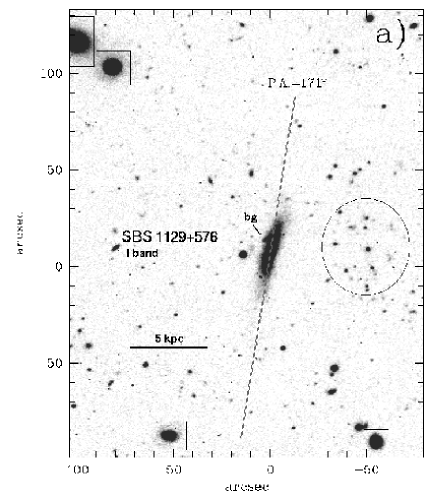
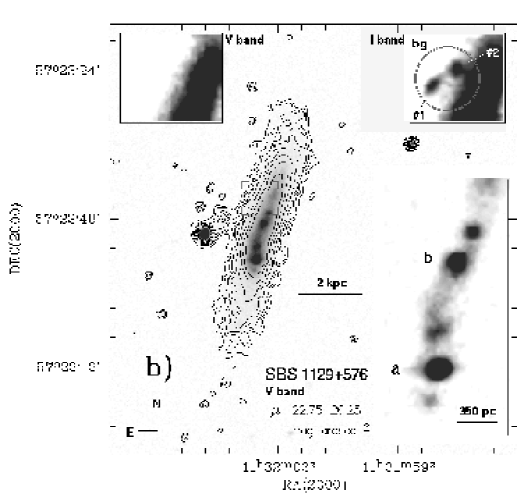
Figure 1: (a) $I$ image of the field around SBS 1129+576. The straight line shows the position of the slit during spectroscopic observations. A pair of red background galaxies intersecting the LSB component $\sim$15″ northwards of the brightest region a (see panel b) is labeled bg. The ellipse delineates the central part of a probable uncatalogued background galaxy cluster. Rectangles mark the position of some other uncatalogued galaxies in the field. These objects span a $(V-I)$ colour range between 1.1 and 1.3 mag. (b) $V$ image of SBS 1129+576. The overlayed contours correspond to surface brightness between 22.75 and 26.25 mag arcsec^-2 in steps of 0.5 mag. The inset to the lower-right, computed from the $V$ image after subtraction of a two-dimensional model for the LSB component, illustrates the spatial distribution of compact star-forming regions. The insets to the upper left and upper right show, respectively, close-up views in the $V$ and $I$ of the region depicted by rectangular brackets. This region shows a smooth morphology in the $V$, while the $I$ image reveals two red ($(V-I)$$\sim$1.6) background galaxies labeled #1 and #2.

SBS 1129+576 ($\alpha$(J2000.0) = 11^h32^m02$\aas@@fstack{s}$5, $\delta$(J2000.0) = +57^∘22′45$\aas@@fstack{\prime\prime}$7, Bicay et al. 2000) was discovered in the course of the Second Byurakan Survey (SBS) (Markarian & Stepanian 1983; Lipovetsky et al. 1988) as a galaxy with strong emission lines, weak continuum and ultraviolet excess seen in a chain of H ii regions embedded within an extended blue low-surface-brightness (LSB) component. Up to now SBS 1129+576 has not been studied in detail. The low metallicity and relatively blue colour of its LSB component (this paper) make it one of the rare young dwarf galaxy candidates (Izotov $\&$ Thuan 1999). In the present paper the physical conditions and chemical abundances of the ionized gas of SBS 1129+576 are studied for the first time. In addition, spectroscopic and $V,I$ photometric data are used to study the properties of the unresolved stellar population in its bright H ii regions and LSB component. Recently Thuan et al. (1999) derived for SBS 1129+576 a redshift $z$ = 0.00522 from single-dish H i 21 cm observations. After correction of the radial velocity for the Virgocentric infall motion, they derive a distance of $D$ = 26.3 Mpc, which we adopt. At this distance 1 arcsec corresponds to a linear scale of 127 pc.

The structure of the paper is as follows. In Sect. 2 we describe the observations and data reduction. The photometric properties of SBS 1129+576 are described in Sect. 3. In Sect. 4 we derive the chemical abundances in the two brightest H ii regions. The properties of the stellar LSB population and its possible age range are discussed in Sect. 5. Finally, Sect. 6 summarises the main conclusions of this work.

2 Observations and data reduction

2.1 Photometric observations and data reduction

Direct images of SBS 1129+576 in $V$ and $I$ (Fig. 1) were acquired with the Kitt Peak 2.1m telescope on April 19, 1999, during a photometric night. The telescope was equipped with a Tektronix 1024$\times$1024 CCD detector operating at a gain of 3 e^- ADU^-1, giving an instrumental scale of 0$\aas@@fstack{\prime\prime}$305 pixel^-1 and field of view of 5′. The total exposures of 20 and 30 min in $V$ and $I$, respectively, were split into four subexposures each being slightly offset with respect to each other for removal of cosmic particle hits and bad pixels. The point spread function in $V$ and $I$ were respectively 1$\aas@@fstack{\prime\prime}$06 and 1$\aas@@fstack{\prime\prime}$17 FWHM. Bias and flat–field images were obtained at the beginning and end of night. Calibration was achieved by observing 4 standard fields from Landolt (Landolt92 (1992)) at 3–4 different airmasses during the night. Our calibration uncertainties are estimated to be 0.01–0.02 mag in each of the $V$ and $I$ bands. The data reduction, including bias subtraction, removal of cosmic particle hits, flat–field correction and absolute flux calibration was made using IRAF.

2.2 Spectroscopic observations and data reduction

The spectroscopic observations were carried out on 19 June, 1999, with the Kitt Peak 4m Mayall telescope and Ritchey-Chretien spectrograph with the T2KB 2048 $\times$ 2048 CCD detector, with the slit at P.A. = 171^∘, centered on the brightest star-forming region and extending along the elongated body of the galaxy (roughly aligned with the major axis; see Fig. 1a). A 2″ $\times$ 300″ slit with the KPC-10A grating in first order and a GG 375 order separation filter was used. The spatial scale along the slit was 0$\aas@@fstack{\prime\prime}$69 pixel^-1 and the spectral resolution $\sim$7 Å (FWHM). The spectra were obtained at an airmass 1.33 and in a total exposure of 60 minutes, which was broken up into 3 subexposures. No correction for atmospheric refraction was made because the slit was oriented with a P.A. close to the parallactic angle. Two Kitt Peak spectrophotometric standard stars were observed for flux calibration. For wavelength calibration, spectra of a He-Ne-Ar comparison lamp were taken after each exposure.

The data reduction was made with the IRAF software package. This includes bias–subtraction, flat–field correction, cosmic-ray removal, wavelength calibration, night sky subtraction, correction for atmospheric extinction and absolute flux calibration of the two–dimensional spectra.

One-dimensional spectra for abundance determination in the two brightest H ii regions a and b (Figs. 1b and 2) were extracted from the two-dimensional spectrum within large apertures of 2″ $\times$ 5″. Some additional spectra of regions a and b within smaller apertures 2″ $\times$ 1$\aas@@fstack{\prime\prime}$1, 2″ $\times$ 1$\aas@@fstack{\prime\prime}$4 and 2″ $\times$ 2$\aas@@fstack{\prime\prime}$1 were also extracted.

In addition we extracted spectra showing hydrogen Balmer absorption lines for five regions along the major axis of the galaxy to study the stellar population of the LSB component. The locations of selected regions, denoted 1 to 5, relative to region a are given in Tables 4 and 5. The spatial extent of these regions along the slit were 6$\aas@@fstack{\prime\prime}$2, 5$\aas@@fstack{\prime\prime}$5, 4$\aas@@fstack{\prime\prime}$8, 4$\aas@@fstack{\prime\prime}$8 and 4$\aas@@fstack{\prime\prime}$8, respectively.

3 Photometric analysis

3.1 Morphology, environment and colour distribution

Table 1: Structural properties of the starburst and LSB components of SBS 1129+576^a.

Band	$\mu_{\rm E,0}$	$\alpha$	$P_{25}$	$m_{P_{25}}$	$E_{25}$	$m_{\rm E_{25}}$	$m_{\rm LSB}$	$m_{\rm SBP}$	$m_{\rm tot}$	$r_{\rm eff}$,$r_{80}$
	mag arcsec-2	pc	kpc	mag	kpc	mag	mag	mag	mag	kpc
(1)	(2)	(3)	(4)	(5)	(6)	(7)	(8)	(9)	(10)	(11)
$V$	21.01$\pm$0.02	436$\pm$4	0.73	18.27	1.59	16.54	16.43	16.23$\pm$0.01	16.22	0.65,1.17
$I$	20.43$\pm$0.03	433$\pm$4	0.78	18.25	1.82	15.92	15.86	15.73$\pm$0.02	15.72	0.69,1.20

^aThe tabulated values have not been corrected for interstellar extinction or inclination.

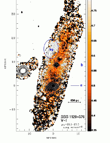
Figure 2: $(V-I)$ map of SBS 1129+576 displayed in the colour range between +0.35 to +0.8 mag. The overlayed contours are from 21.1 to 25.0 $V$ mag arcsec^-2 in steps of 0.3 mag. The region, depicted by the ellipse, shows a strikingly redder $(V-I)$ colour ($\sim$ 1.6 mag) than the average colour $\sim$ 0.56 mag of the LSB component. This local maximum in the $(V-I)$ colour is to be attributed to background galaxies labeled bg in Fig. 1a and in the upper-right inset of Fig. 1b.

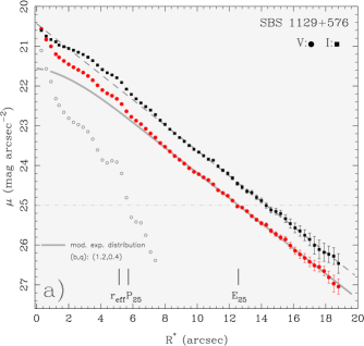
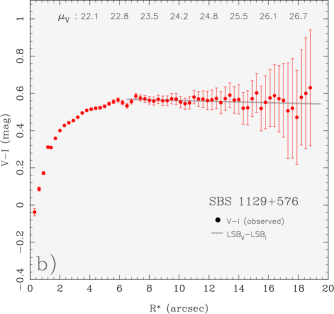
Figure 3: (a) Surface brightness profiles (SBP) of SBS 1129+576 in the $V$ and $I$ derived using the method iii. The modeled surface brightness distribution of the LSB component in the $V$ assuming a modified exponential distribution with ($b$,$q$)=(1.2,0.4) is shown by the thick-grey curve. Open circles show the surface brightness distribution of the light in excess to the modeled LSB profile and is to be attributed to the compact star-forming regions along the major axis of the galaxy (Fig. 1b). The effective radius $r_{\rm eff}$ of the $V$ SBP and the isophotal radii $P_{25}$ and $E_{25}$ of, respectively, the starburst and the LSB component at 25 $V$ mag arcsec^-2 are indicated. The dashed line shows a linear fit to the $I$ band profile for $R^{*}\geq$8″, extrapolated to $R^{*}$ = 0. (b) Circles show the  $(V-I)$ colour profile computed by subtraction of the SBPs displayed in the left panel. Labels attached to the upper axis indicate the $V$ surface brightness corresponding to the respective photometric radius $R^{*}$. The $(V-I)$ colour distribution (thick-grey line) is obtained by subtraction of the fits in $V$ and $I$ shown in (a). It closely matches the observed colour distribution and implies a practically constant $(V-I)$ colour of $\approx$ 0.56 mag over a range of 4 magnitudes in surface brightness.

SBS 1129+576 appears as an oblate dwarf ($M_{V}$ $\sim$ –15.9 mag) galaxy with a projected axial ratio of 4 at 25 $V$ mag arcsec^-2 (Fig. 1, 2). Star formation activity takes place in the central parts of the galaxy within an elongated, moderately blue region with a size of $\sim$ 2.5 kpc. The $V$ magnitudes of regions a and b are respectively $\approx$ 19.0 mag and 20.0 mag, corresponding to absolute $V$ magnitudes –13.1 mag and –12.1 mag. The $(V-I)$ colours of $\sim$ 0.1 mag and $\sim$ 0.3 mag, respectively, of regions a and b are relatively blue. The $(V-I)$ colour of the LSB component shows a smooth change from $\sim$ 0.44 mag in the immediate vicinity of region a to an average colour of $\sim$ 0.56 $\pm$ 0.03 mag in the outer part of the galaxy (see Fig. 3b). The $(V-I)$ colour map (Fig. 2) reveals for surface brightness levels fainter than 24 $V$ mag arcsec^-2, a featureless and relatively constant colour over the whole LSB component except for a strikingly red ($(V-I)$ $\sim$ 1.6 mag) region located $\sim$ 15″ north of region a (region $bg$ in Figs. 1 and 2). The local colour excess observed in region $bg$ is due to two background galaxies seen in the $I$ image only. A close-up view of this region in the $V$ and $I$ is shown in the upper insets of Fig. 1b. A potential slight overestimate of the $(V-I)$ colour of the LSB component in SBS 1129+576 as a result of the superposition of background sources at different locations is likely given the numerous red ($(V-I)$ $>$ 1.2 mag) faint ($m_{I}$ $\ga$ 20.5 mag) sources in the field of the galaxy. Figure 1a shows that SBS 1129+576 is located in front of a probable background cluster of galaxies centered $\sim$ 50″ west of region a. This cluster with the central part delineated by the ellipse as well as several red galaxies indicated by rectangles in Fig. 1a are not catalogued in the NASA/IPAC Extragalactic Database (NED).

3.2 Surface photometry

Surface brightness profiles (SBPs) of SBS 1129+576 have been computed following the methods i through iii described in Papaderos et al. (1996a ). Briefly, the photometric radius $R^{*}=(A(\mu)/\pi)^{0.5}$ corresponding to the surface brightness level $\mu$ is computed from the area $A(\mu)$ of a galaxy in arcsec², as derived through ellipse fitting or computation of a line-integral along an isophote (methods i and ii) or summation of all pixels inside a polygonal aperture with a surface brightness brighter than $\mu$ (method iii). Essentially, these techniques trace the growth of the isophotal size of a galaxy with decreasing intensity $I$. They require no choice of a “geometrical center” of a galaxy and insure that the photometric radius $R^{*}$ is a monotonic function of $\mu$. Evidently, in order to derive SBPs as described above, one has to keep track of the morphology of a BCD throughout its intensity span, i.e. in general to be able to interpolate an isophote down to the faintest measured level $\mu$ of a SBP. This allows to visually check for and screen-out foreground and background sources in the periphery of the galaxy, thus to make sure that source confusion does not affect the SBP slope at faint intensity levels. This task is more difficult to achieve when computing SBPs based on photon statistics inside circular or elliptical annuli, extending out to a user-defined maximal radius $r_{\rm max}$. Especially for BCDs, SBPs derived with the latter methods may considerably vary, depending on subjective assumptions on the $r_{\rm max}$ or the “center” of a galaxy.

As a check for consistency, we also computed SBPs using method iv in Papaderos et al. (papaderos02 (2002)). This technique is based on the calculation of photon statistics for a series of masks of arbitrary (generally irregular) shape, mapping equidistant logarithmic intensity intervals between $I_{\rm min}$ and $I_{\rm max}$. As in methods i through iii, method iv does not require the choice of a “geometrical center” and accounts adequately for the large morphological variation of a BCD, with a typically smooth LSB part and an irregular star-forming component.

We derived $V$ and $I$ SBPs from the total light of the galaxy, except for region bg (shown by the ellipse in Fig. 2) which has been replaced by a two-dimensional fit to the adjacent LSB emission. Both SBPs in Fig. 3a are derived using the method iii. They show an exponential intensity decrease for radii $R^{*}\ga 8$″ with a scale length $\alpha\approx$3$\aas@@fstack{\prime\prime}$4. That the exponential model yields a reasonable approximation to the LSB emission is also indicated from fitting a Sérsic (sersic68 (1968)) profile

$$I(R^{*})=I_{0}\,\exp\left(-\frac{R^{*}}{\beta}\right)^{\eta}$$ (1)

(see also Caon et al. Caon93 (1993), Cellone et al. cellone94 (1994), Papaderos et al. 1996a ) to the radius interval $R^{*}\geq$8″. The exponent $\eta$ obtained this way, respectively 1.2 and 1.1 in $V$ and $I$, is marginally larger than the value $\eta$ = 1, corresponding to the exponential law.

However, a closer inspection of the $I$ band SBP (Fig. 3a) shows that an inwards extrapolation of the exponential law fitted to the LSB component (see dashed line, overlayed with the $I$ profile) predicts for small radii ($R^{*}$$\la$2″) a slightly higher intensity than the one observed. Such a pure exponential LSB model would imply that the star-forming component in SBS 1129+576 provides no more than 5% of the total $I$ emission and that its contribution decreases rapidly at small radii. This suggests that the stellar LSB emision of SBS 1129+576 is best approximated by an exponential profile with a flattening in its inner part. Note that such SBPs have been frequently observed in dwarf ellipticals (e.g., Binggeli & Cameron binggeli91 (1991)), dwarf irregulars (Rönnback & Bergvall 1994; Patterson & Thuan patterson96 (1996); Makarova m99 (1999); van Zee v2000 (2000)) and a few blue compact dwarf (BCD) galaxies (e.g., Papaderos et al. 1996a ; Vennik et al. vennik96 (1996), vennik00 (2000); Telles & Terlevich telles97 (1997); Guseva et al. Guseva2001 (2001); Fricke et al. Fricke00 (2001)). SBPs of this kind, classified “type V” in Binggeli & Cameron (binggeli91 (1991)), can be approximated by, e.g., the modifed exponential distribution proposed in Papaderos et al. (1996a ):

$$I(R^{\star})=I_{\rm E,0}\exp\left(-\frac{R^{\star}}{\alpha}\right)\{1-q\exp(-P_{3}(R^{\star}))\}$$ (2)

with

$$P_{3}(R^{\star})=\left(\frac{R^{\star}}{b\alpha}\right)^{3}+\left(\frac{R^{\star}}{\alpha}\frac{1-q}{q}\right).$$ (3)

The empirical fitting function (Eq. 2) flattens with respect to the exponential law inside of a cutoff radius $b\alpha$, and attains at $R^{*}$=0″ an intensity given by the relative depression parameter $q=\Delta I/I_{\rm E,0}<1$. An advantage of Eq. 2 is that its exponential part, depending on $I_{E,0}$ and $\alpha$ only, can be readily constrained from linear fits to the outer exponential part of a “type V” SBP.

In order to disentangle the intensity distribution of the LSB component and better constrain the depression parameters $b$ and $q$ in Eq. 2 we follow the approach adopted in Guseva et al. (Guseva2001 (2001)). We first subtracted compact (diameter $\la$4″) high-surface-brightness regions in the inner part of the galaxy and then rederived SBPs from the residual underlying LSB emission. Fitting Eq. 2 to the resulting profiles yields $V$ and $I$ depression parameters ($b$,$q$) = (1.2,0.4) and an exponential scale length $\alpha$ $\sim$ 430 pc. In Fig. 3a we show for the $V$ SBP the modeled surface brightness distribution of the LSB component according to Eq. 2 and the emission in excess of the model with the thick-grey curve and open circles, respectively. The dashed line shows a linear fit to the $I$ band profile for $R^{*}\geq$8″, extrapolated to $R^{*}$ = 0. The excess emission is due to the chain of compact star-forming regions along the major axis of the galaxy.

Figure 4: The KPNO 4m spectra of regions a and b with the emission lines identified. The lower spectra in (a) and (b) are the observed spectra downscaled by a factor of 15.

Table 1 summarizes the derived photometric quantities. Cols. 2 and 3 give, respectively, the central surface brightness $\mu_{\rm E,0}$ and scale length $\alpha$ of the LSB component as obtained from linear fits to the SBPs for $R^{*}\geq 8$″ and weighted by the photometric uncertainty of each point. These quantities correspond to the values one would obtain from extrapolation of the exponential slope observed in the outlying regions of the galaxy to $R^{*}=0$. Cols. 4 through 8 list quantities obtained from profile decomposition where the intensity distribution of the LSB component was modeled by the modified exponential distribution (Eq. 2). Cols. 4 and 6 give the radial extent $P_{25}$ and $E_{25}$ of the starburst and LSB components, respectively, both determined at a surface brightness 25 mag arcsec^-2. The apparent magnitudes of both components within $P_{25}$ and $E_{25}$ are listed in cols. 5 and 7, respectively. Col. 8 gives the apparent magnitude of the LSB component in each band within a photometric radius of 18″, as derived from integration of the modeled distribution (Eq. 2). The total magnitudes of the galaxy, as inferred from SBP integration out to the same radius and by integrating the flux within a polygonal aperture are listed in cols. 9 and 10, respectively. Col. 11 gives the effective radius $r_{\rm eff}$ and the radius $r_{80}$ which encircles 80% of the galaxy’s total flux.

From Table 1 it is evident that the integrated emission of the starburst component including the two brightest regions a and b contributes only $\sim$ 17% of the $V$ light of SBS 1129+576 within its 25 $V$ mag arcsec^-2 isophote. This is a factor of 3 lower than the average of 50% derived for BCDs in the $B$ band by Papaderos et al. (1996b ) and Salzer & Norton (SN99 (1999)).

The $(V-I)$ colour profile of SBS 1129+576, derived from subtraction of the corresponding SBPs, is shown in Fig. 3b. Its behaviour is similar to that in BCDs (Papaderos et al. 1996a ) and compact irregular dwarf galaxies (Patterson $\&$ Thuan patterson96 (1996); van Zee v2000 (2000)) with a blue colour in the inner part of the galaxy and a redder, relatively constant colour at larger radii. The colour in SBS 1129+576 increases gradually from $(V-I)$ $\la$ 0.2 mag for radii $R^{*}$ $\la$ 2″ to $\sim$ 0.5 mag at $R^{*}$ $\la$ 5″ and remains practically constant at $\sim$ 0.56 $\pm$ 0.03 mag in the outer part of the galaxy. The observed colour is in accord with the one resulting from subtraction of the apparent magnitudes of the modeled distributions for the LSB component (Table 1, col. 8) which has an average value of 0.57 mag.

4 Chemical abundances

In this Section we analyze the element abundances in SBS 1129+576 based on spectroscopic observations of the two brightest H ii regions a and b. The spectra of these star-forming regions (Fig. 4) are characterised by strong nebular emission lines superposed on stellar Balmer absorption lines. The latter are also seen along the slit in the LSB component.

Table 2: Observed ($F$($\lambda$)) and corrected ($I$($\lambda$)) fluxes and equivalent widths ($EW$) of emission lines in regions a and b.

	region a				region b
$\lambda_{0}$(Å) Ion	$F$($\lambda$)/$F$(H$\beta$)	$I$($\lambda$)/$I$(H$\beta$)	$EW$(Å)		$F$($\lambda$)/$F$(H$\beta$)	$I$($\lambda$)/$I$(H$\beta$)	$EW$(Å)
3727 [O ii]	1.408 $\pm$0.035	1.346 $\pm$0.037	51.0 $\pm$0.8		1.875 $\pm$0.061	1.758 $\pm$0.065	38.8 $\pm$0.7
3835 H9	0.030 $\pm$0.013	0.084 $\pm$0.048	1.0 $\pm$0.4		…	…	…
3868 [Ne iii]	0.169 $\pm$0.015	0.161 $\pm$0.015	4.5 $\pm$0.4		0.313 $\pm$0.026	0.293 $\pm$0.026	5.3 $\pm$0.4
3889 H8 + He i	0.128 $\pm$0.014	0.179 $\pm$0.026	4.2 $\pm$0.5		0.147 $\pm$0.025	0.240 $\pm$0.051	3.1 $\pm$0.5
3968 [Ne iii] +H7	0.122 $\pm$0.012	0.177 $\pm$0.024	3.7 $\pm$0.4		0.158 $\pm$0.027	0.249 $\pm$0.052	3.3 $\pm$0.6
4101 H$\delta$	0.183 $\pm$0.013	0.235 $\pm$0.023	5.5 $\pm$0.4		0.180 $\pm$0.020	0.252 $\pm$0.044	3.5 $\pm$0.4
4340 H$\gamma$	0.457 $\pm$0.018	0.490 $\pm$0.024	15.6 $\pm$0.5		0.434 $\pm$0.026	0.483 $\pm$0.038	9.1 $\pm$0.5
4363 [O iii]	0.061 $\pm$0.014	0.058 $\pm$0.014	1.7 $\pm$0.4		0.117 $\pm$0.023	0.110 $\pm$0.023	2.2 $\pm$0.4
4471 He i	0.033 $\pm$0.014	0.032 $\pm$0.014	1.0 $\pm$0.4		0.042 $\pm$0.019	0.038 $\pm$0.019	0.8 $\pm$0.3
4861 H$\beta$	1.000 $\pm$0.027	1.000 $\pm$0.030	41.0 $\pm$0.8		1.000 $\pm$0.040	1.000 $\pm$0.045	25.4 $\pm$0.8
4959 [O iii]	0.666 $\pm$0.022	0.637 $\pm$0.022	24.4 $\pm$0.6		1.173 $\pm$0.044	1.099 $\pm$0.044	26.6 $\pm$0.7
5007 [O iii]	1.975 $\pm$0.045	1.888 $\pm$0.045	73.8 $\pm$0.9		3.252 $\pm$0.099	3.049 $\pm$0.099	76.9 $\pm$1.0
5876 He i	0.086 $\pm$0.010	0.082 $\pm$0.010	4.5 $\pm$0.5		0.093 $\pm$0.017	0.087 $\pm$0.017	3.0 $\pm$0.6
6300 [O i]	0.048 $\pm$0.010	0.046 $\pm$0.010	3.0 $\pm$0.6		0.075 $\pm$0.017	0.069 $\pm$0.017	3.1 $\pm$0.7
6563 H$\alpha$	2.692 $\pm$0.058	2.599 $\pm$0.064	186.3 $\pm$1.8		2.662 $\pm$0.079	2.526 $\pm$0.088	137.3 $\pm$1.6
6584 [N ii]	0.041 $\pm$0.008	0.039 $\pm$0.008	2.8 $\pm$0.5		0.071 $\pm$0.013	0.066 $\pm$0.013	3.1 $\pm$0.6
6678 He i	0.030 $\pm$0.008	0.029 $\pm$0.008	2.1 $\pm$0.6		0.026 $\pm$0.015	0.024 $\pm$0.015	1.1 $\pm$0.7
6717 [S ii]	0.142 $\pm$0.010	0.136 $\pm$0.010	10.1 $\pm$0.7		0.168 $\pm$0.018	0.155 $\pm$0.018	7.5 $\pm$0.8
6731 [S ii]	0.103 $\pm$0.010	0.098 $\pm$0.010	7.3 $\pm$0.7		0.114 $\pm$0.015	0.106 $\pm$0.015	5.1 $\pm$0.6
$C$(H$\beta$) dex	0.000$\pm$0.028				0.000$\pm$0.041
$F$(H$\beta$)a	0.50$\pm$0.01				0.23$\pm$0.01
$EW$(abs) Å	1.9$\pm$0.4				1.7$\pm$0.4

^ain units 10^-14 erg s^-1cm^-2.

The emission line fluxes were measured using Gaussian profile fitting. The errors of the line flux measurements include the errors in the fitting of profiles and those in the placement of the continuum. They have been propagated in the calculations of the elemental abundance errors. The observed ($F$($\lambda$)) and corrected ($I$($\lambda$)) emission line fluxes relative to the H$\beta$ fluxes, the equivalent widths $EW$ of the emission lines, the observed fluxes of H$\beta$, and the equivalent widths of the hydrogen absorption lines are listed in Table 2.

The H$\alpha$-to-H$\beta$ flux ratios in both H ii regions are lower than the theoretical value (e.g., Brocklehurst 1971). This is likely not due to data reduction problems as the H$\alpha$-to-H$\beta$ flux ratios in other galaxies observed during the same night are greater than the theoretical ones. Therefore, an extinction coefficient $C$(H$\beta$)=0 was assumed for these H ii regions and the emission-line fluxes were corrected for Balmer line absorption only.

Some diagnostic lines were studied to check for possible deviations of the H ii region emission in SBS 1129+576 from the predictions of photoionization models. For this purpose, data for the emission lines were collected for the galaxies from Izotov et al. (ITL94 (1994), Izotov97 (1997)), Thuan et al. (til95 (1995)), Izotov & Thuan (IT98a (1998)), Fricke et al. (Fricke00 (2001)), Noeske et al. (Noeske00 (2000)), and Guseva et al. (Guseva2001 (2001)). In total we use data for 46 star-forming galaxies: 11 lowest-metallicity galaxies with an oxygen abundance 12 + log(O/H) $\leq$ 7.6 and 35 higher-metallicity galaxies with an oxygen abundance 12 + log(O/H) $\geq$ 7.9. Various emission line flux ratios are shown in Fig. 5.

Figure 5: Dependence on a logarithmic scale of the line flux ratios (a) log([N ii]$\lambda$6584/H$\alpha$) and (b) log([O i]$\lambda$6300/H$\alpha$) on the log([O ii]$\lambda$3727/[O iii]$\lambda$5007) ratio. Data for galaxies with 12 + log(O/H) $\leq$ 7.6 and 12+log(O/H) $\geq$ 7.9 are shown by filled and open circles, respectively. The positions of the brightest regions a and b in SBS 1129+576 are shown by triangles. Thin and thick solid lines represent theoretical predictions from photoionization models calculated with the CLOUDY code for ionizing stars with effective temperatures $T_{\rm eff}$ = 45 000 K and $T_{\rm eff}$ = 50 000 K and a heavy element mass fraction $Z$ = $Z_{\odot}$/36. Dot-dashed and dashed lines correspond to models with $T_{\rm eff}$ = 50 000 K and a heavy element mass fractions $Z$ = $Z_{\odot}$/20 and $Z_{\odot}$/5, respectively. The ionization parameter decreases from log $U$ = –2.0 (left) to log $U$ = –3.0 (right).

In this figure, galaxies with low and high oxygen abundances split into two sequences, shown by filled and open circles, respectively. This separation is in overall agreement with photoionization H ii region models. However, regions a and b of SBS 1129+576 (filled triangles in Fig. 5) having lower ionization parameters, lie outside the main location of low-metallicity galaxies. The line ratios [S ii]$\lambda$6717+6731/H$\alpha$ and [N ii]$\lambda$6584/H$\alpha$ in SBS 1129+576 are $\sim$ 3 times and [O i]$\lambda$6300/H$\alpha$ $\sim$ 5 times higher than the ones in the sample of the 11 lowest-metallicity galaxies. The locations of regions a and b in Fig. 5 also significantly deviate from the model predictions calculated with the CLOUDY code (Ferland F96 (1996); Ferland et al. F98 (1998)) for a heavy element mass fraction $Z$ = $Z_{\odot}$/36 derived for region a and for ionizing stars with effective temperatures of $T_{\rm eff}$ = 45 000 K (thin solid lines) and $T_{\rm eff}$ = 50 000 K (thick solid lines). By dot-dashed and dashed lines we also show the model predictions for $T_{\rm eff}$ = 50 000 K and two heavy element mass fractions of $Z_{\odot}$/20 and $Z_{\odot}$/5, respectively.

The discrepancies between photoionization models and the observed line intensity ratios (essentially the high [O i]$\lambda$6300/H$\beta$ and [S ii]$\lambda$6717+6731/H$\beta$) are usually explained by some contribution of shock waves. However, Stasińska & Izotov (StasinskaIz02 (2003)) from the analysis of a large sample ($\sim$ 400) of H ii galaxies proposed another model to explain the enhancement of these lines in low-metallicity H ii regions by invoking chemical inhomogeneities and self-enrichment by the heavy elements. Their models take into account the time evolution of an ionizing cluster in the simple case of an expanding bubble. The models predict an increase of the [O i]$\lambda$6300/H$\beta$ ratio in better agreement with observations of low-metallicity H ii regions. Nevertheless, the hypothesis of shock heating may also be considered as an alternative explanation.

A two-zone photoionized H ii region model has been assumed for the abundance determination. The electron temperature $T_{\rm e}$(O iii) in the high-ionization region has been derived from the observed flux ratio [O iii]$\lambda$4363/($\lambda$4959+5007), using a five-level atom model (Aller Aller84 (1984)) with atomic data from Mendoza (Mendoza83 (1983)). The electron temperature $T_{\rm e}$(O ii) in the low-ionization region has been obtained using the empirical relation between $T_{\rm e}$(O ii) and $T_{\rm e}$(O iii) from the H ii region photoionization models by Stasińska (Stasinska90 (1990)). The [S ii]$\lambda$6717/$\lambda$6731 ratio was used to derive the electron number density $N_{\rm e}$(S ii).

The abundances of O⁺², Ne⁺² and He⁺ were derived applying the electron temperature $T_{\rm e}$(O iii). The electron temperature $T_{\rm e}$(O ii) is adopted for the O⁺ and N⁺ ionic abundance determination.

The total oxygen abundance is the sum of the O⁺ and O⁺² abundances. The total abundances of other heavy elements were derived using ionization correction factors following Izotov et al. (ITL94 (1994), Izotov97 (1997)) and Thuan et al. (til95 (1995)). The ionic and heavy element abundances for regions a and b together with electron temperatures and electron number densities are given in Table 3 along with the adopted ionization correction factors (ICF).

The oxygen abundances 12 + log(O/H) = 7.36 $\pm$ 0.10 ($Z$=$Z_{\odot}$/36) and 7.48 $\pm$ 0.12 ($Z$=$Z_{\odot}$/28) for regions a and b, respectively, are slightly different but still consistent within the 1$\sigma$ errors. Note that the oxygen abundance in region a may be underestimated due to the additional contribution of shock enhancement of the [O iii]$\lambda$4363 emission line. Such an effect can be present in region b, but it is expected to be much larger in region a with the much weaker [O iii]$\lambda$4363 emission line (Table 2).

The abundance ratios of nitrogen and neon to oxygen (Table 3) are in agreement with those derived in other lowest-metallicity dwarf galaxies (Izotov & Thuan IT99 (1999)).

The low metallicity of SBS 1129+576 makes it potentially suitable for He abundance determination. For this, we use the three strongest He i $\lambda$4471, $\lambda$5876 and $\lambda$6678 emission lines. The helium abundance derived from the corrected fluxes of all observed He i emission lines is shown in Table 3. The mean values for the He mass fraction of $Y$ = 0.220 $\pm$ 0.027 (region a) and $Y$ = 0.202 $\pm$ 0.042 (region b), though formally consistent, are significantly lower than the primordial He mass fraction $Y_{\rm p}$ = 0.244 $\pm$ 0.002, derived by extrapolating the $Y$ vs O/H linear regression to O/H = 0 for the sample of 45 low-metallicity dwarf galaxies (Izotov & Thuan IT98a (1998)), or to $Y_{\rm p}$ = 0.245 $\pm$ 0.002 derived for the most metal-deficient BCDs I Zw 18 and SBS 0335–052 (Izotov et al. ICFGGT99 (1999)).

The likely source of lower values of $Y$ in SBS 1129+576 is underlying stellar He i absorption superposed on the He i emission lines. Comparing the equivalent widths of He i emission lines (Table 2) with those predicted by population synthesis models for He i absorption lines (e.g., González Delgado et al. 1999) we conclude that underlying stellar absorption can decrease the fluxes of the He i emission lines by as much as $\sim$ 10 – 20% for He i $\lambda$5876 (assuming the equivalent widths of He i $\lambda$5876 and He i $\lambda$4471 absorption lines to be similar) and more for other He i lines. Hence, despite its low metallicity SBS 1129+576 is not a good candidate for primordial helium abundance determination because of the large effect of the underlying stellar absorption.

Table 3: Element abundances in regions a and b.

Value	region a		region b
$T_{\rm e}$(O iii)(K)	18930$\pm$2540		20560$\pm$2660
$T_{\rm e}$(O ii)(K)	15350$\pm$1930		15850$\pm$2180
$T_{\rm e}$(S iii)(K)	17410$\pm$2110		18760$\pm$2210
$N_{\rm e}$(S ii)(cm-3)	40$\pm$120		10$\pm$10
O+/H+($\times$105)	1.092$\pm$0.351		1.298$\pm$0.594
O+2/H+($\times$105)	1.215$\pm$0.378		1.691$\pm$0.907
O/H($\times$105)	2.307$\pm$0.516		2.989$\pm$1.084
12 + log(O/H)	7.363$\pm$0.097		7.476$\pm$0.121
N+/H+($\times$107)	2.785$\pm$0.896		5.699$\pm$2.021
ICF(N)a	2.11		2.30
log(N/O)	–1.593$\pm$0.241		–1.414$\pm$0.298
Ne+2/H+($\times$105)	0.213$\pm$0.070		0.320$\pm$0.165
ICF(Ne)a	1.90		1.77
log(Ne/O)	–0.756$\pm$0.199		–0.722$\pm$0.245
He+/H+($\lambda$4471)	0.0686$\pm$0.0313		0.0819$\pm$0.0399
He+/H+($\lambda$5876)	0.0684$\pm$0.0094		0.0603$\pm$0.0142
He+/H+($\lambda$6678)	0.0868$\pm$0.0251		0.0692$\pm$0.0447
He+/H+
(weighted mean)	0.0705$\pm$0.0085		0.0633$\pm$0.0129
He/H	0.0705$\pm$0.0085		0.0633$\pm$0.0129
$Y$	0.2199$\pm$0.0271		0.2019$\pm$0.0418

^aICF is the ionization correction factor.

5 Age of the underlying stellar population

The low metallicity and relatively blue $(V-I)$ colour of SBS 1129+576 make this object a good young galaxy candidate. In this section we consider the properties of the stellar populations in the galaxy and discuss its evolutionary status. The observed properties of stellar populations are dependent on the metallicity and star formation history. They also can be influenced by interstellar extinction and emission of the ionized gas. Therefore, we use all available spectroscopic and photometric observational data on 5 LSB regions to put consistent constraints on the age of stellar populations in SBS 1129+576.

Emission and absorption hydrogen Balmer lines are seen in the spectra of a large part of the galaxy along the slit. This allows us to study the age of stellar populations, using two methods, based on the time evolution of equivalent widths of (1) nebular emission Balmer lines and (2) stellar absorption Balmer lines. The advantage of these methods is that they are extinction-insensitive. This is very important because the only way to derive interstellar extinction from optical spectra is to compare observed and theoretical decrements of Balmer emission lines. However, in the extended low-intensity regions the emission lines are weak or absent, making estimates of the interstellar extinction uncertain.

The age of the stellar population in a galaxy can be obtained from a third method, comparing the observed and theoretical spectral energy distributions (SED), the latter computed with various ages and histories of star formation for the stellar population. However, the shape of the observed continuum is dependent on both age and interstellar extinction. If no other information on the stellar population is available (e.g., the age derived from hydrogen equivalent widths), the extinction coefficient is set equal to zero (for a spectrum with no Balmer emission lines), and the age can simply be inferred by fitting the observed spectrum with theoretical SEDs. This method gives a maximum age among possible age estimates. If, on the other hand, the ages of stellar populations can be estimated by some other methods, then the reddening can be derived from the SEDs.

Finally, to study stellar populations in SBS 1129+576, we use broad-band photometry. However, similar to the SED fitting method, extinction also affects age determination based on photometric data. Additionally, ionized gas emission can significantly influence both the observed SEDs and broad-band colours.

Figure 6: Distributions of the H$\alpha$ equivalent width on a logarithmic scale (thick dashed line), and fluxes of the H$\alpha$ (thick solid line), H$\beta$ (thin solid line), [O iii] $\lambda$5007 (thin dashed line) emission lines and the continuum near H$\beta$ (dotted line) along the major axis of SBS 1129+576. The axis origin is set to the position of region a (see Fig. 1). The fluxes are in arbitrary units.

Before dealing with stellar populations, we first consider how important is the contribution of ionized gas emission to the total light. The variations of the equivalent width of the H$\alpha$ emission line and the fluxes of the strongest emission lines along the major axis of SBS 1129+576 are shown in Fig. 6. The maximum $EW$(H$\alpha$) = 385Å and $EW$(H$\beta$) = 64 Å are derived in region a. The lower $EW$(H$\alpha$) and $EW$(H$\beta$) for these regions listed in Table  2 are due to different apertures used, of 5″$\times$2″ (Table 2) and of 0$\aas@@fstack{\prime\prime}$69$\times$2″ (Fig. 6). The H$\alpha$ equivalent widths in other regions are much lower. Hence, the contribution of gaseous emission to broad-band fluxes is small in the bright H ii regions and negligible in the LSB component.

5.1 Age from Balmer nebular emission lines

The largest equivalent widths $EW$(H$\alpha$) are measured in regions a and b (Fig. 6), implying that the light from these regions is dominated by young stellar populations. The equivalent widths of H$\alpha$, H$\beta$ emission lines in LSB regions are much smaller, implying a higher contribution to the light of the old stellar populations. The fluxes and equivalent widths of the H$\alpha$, H$\beta$ (and H$\gamma$ where possible) emission lines were measured in the spectra of five LSB regions and listed together with errors in Table 4. Because the H$\beta$ emission line is narrower than the absorption line and does not fill the absorption component, its flux was measured using the continuum level at the bottom of the absorption line. This level has been chosen by visually interpolating from the absorption line wings to the center of the line.

The extinction cannot be derived from the Balmer decrement because the observed H$\alpha$-to-H$\beta$ emission line flux ratios for most of the selected regions are lower than theoretical predictions of ionization-bounded H ii region models (Tables 2, 4 and Fig. 7). Therefore an extinction coefficient $C$(H$\beta$) of zero is adopted. Two dashed lines in Fig. 7 denote the theoretical values $F$(H$\alpha$)/$F$(H$\beta$) = 2.86 for $T_{\rm e}$ = $10^{4}$ K and 2.75 for $T_{\rm e}$ = 2 $\times$ $10^{4}$ K. H$\alpha$ and H$\beta$ fluxes have been measured in each region except for the outermost regions 1 and 5 where only H$\alpha$ emission is present. Only in the two regions, 2 and 4, is the H$\alpha$/H$\beta$ flux ratio larger than the theoretical recombination flux ratio. No correction for the absorption line equivalent width has been made in these regions. The extinction coefficients $C$(H$\beta$) for regions 2 and 4 are shown in Table 4. Note that $C$(H$\beta$) for region 4 is very uncertain, because of the very low equivalent width $EW$(H$\beta$), which is comparable to the $EW$ of the H$\beta$ absorption line.

Figure 7: The observed H$\alpha$/H$\beta$ emission line flux ratios in the different regions of SBS 1129+576. Solid horizontal bars indicate the apertures wherein the spectra were extracted. Large circles show the H$\alpha$/H$\beta$ flux ratios for regions a and b, computed within different apertures. The position of the centers of the two brightest H ii regions is marked by vertical solid lines. Small circles show the same ratios for the fainter regions 2, 3 and 4. The upper and lower dashed horizontal lines denote the theoretical $F$(H$\alpha$)/$F$(H$\beta$) flux ratios for ionization-bounded (case B) H ii regions with $T_{\rm e}$ = $10^{4}$ K and $T_{\rm e}$ = 2 $\times$ $10^{4}$ K, respectively.

The dependence of the H$\alpha$ emission line equivalent width on age is shown in Fig. 8. Here we assume ionization-bounded H ii region model. The model H$\alpha$ equivalent widths in the case of density-bounded H ii region are lower than those in Fig. 8. Since the temporal evolution of emission line equivalent widths depends on the star formation history we consider two limiting cases: an instantaneous burst model and models with continuous star formation. The instantaneous burst model equivalent widths of H$\alpha$ and H$\beta$ emission lines are calculated using the galactic evolution code PEGASE.2 (Fioc & Rocca-Volmerange F97 (1997)). In Fig. 8 the $EW$(H$\alpha$) for the heavy element mass fraction $Z_{\odot}$/50 is shown by a solid line and that for the heavy element mass fraction $Z_{\odot}$/20 by a dashed line. PEGASE.2 is based on the Padua stellar evolutionary models (Bertelli et al. Bertelli94 (1994)) and stellar atmosphere models from Lejeune et al. (Lejeune98 (1998)). An initial mass function with a Salpeter slope ($\alpha$ = –2.35), and upper and lower mass limits of 120 $M_{\odot}$ and 0.1 $M_{\odot}$ are adopted for all our calculations with the PEGASE.2 code.

An instantaneous burst model is most appropriate for the star-forming regions a and b. The maximum equivalent widths of Balmer emission lines in region a ($EW$(H$\alpha$) = 385Å and $EW$(H$\beta$) = 64 Å) are consistent with an instantaneous burst age of 6 Myr for a heavy element mass fraction of $Z$ = $Z_{\odot}$/20 and of 9 Myr for $Z$ = $Z_{\odot}$/50 (Fig. 8). The maximum value $EW$(H$\alpha$) = 180Å for region b is consistent with an instantaneous burst age of 9 Myr for $Z$ = $Z_{\odot}$/20 and 11 Myr for $Z$ = $Z_{\odot}$/50. The $EW$s of Balmer emission lines in regions a and b are probably slightly underestimated due to the significant ($\ga$ 30%; Fig. 3a) line-of-sight contribution of the emission from the LSB component at the respective position. Given the steep decrease of the $EW$(H$\alpha$) as a function of time for 7 $\la$ log($t$ yr) $\la$ 7.4 (Fig. 8) this will not significantly reduce the instantaneous burst age for regions a and b.

In continuous star formation models we adopt a constant star formation rate in the interval between the time $t_{\rm i}$ when star formation starts and $t_{\rm f}$ when it stops. Time is zero now and increases to the past.

We use the model equivalent widths of hydrogen emission lines and SEDs for instantaneous bursts (Fioc & Rocca-Volmerange F97 (1997)) to calculate the temporal evolution of the equivalent widths of hydrogen emission lines in the case of continuous star formation with the constant SFR. The results are given in Fig. 8 for a heavy element mass fraction $Z_{\odot}$/20. The temporal dependence of the equivalent width of the H$\alpha$ emission line is shown for continuous star formation starting at time $t_{\rm i}$, as defined by the abscissa value, and stopping at $t_{\rm f}$ = 5 Myr (dotted line) and $t_{\rm f}$ = 8 Myr (dash-dotted line). The equivalent width of the H$\alpha$ emission line in the spectrum of a stellar population formed between $t_{\rm i}$ and $t_{\rm f}$ is the value of $EW$ at time $t_{\rm i}$ (Fig. 8). At a fixed $EW$, the younger are the youngest stars, the larger is the time interval $t_{\rm i}-t_{\rm f}$, i.e. the older are the oldest stars.

The models of the continuous star formation apply best to the extended stellar component in SBS 1129+576. The observed $EW$(H$\alpha$) for regions 1 – 5 (Table 4) are shown in Fig. 8 by triangles on the theoretical curve with the star formation stopping at $t_{\rm f}$ = 8 Myr ago and correspond to ages $t_{\rm i}$ in the range 20 – 400 Myr. If instead the star formation continues until $t_{\rm f}$ = 5 Myr (dotted line), then the age $t_{\rm i}$ of the oldest stars, as derived from the equivalent widths of the H$\alpha$ and H$\beta$ emission lines, should be in the range 50 Myr – 5 Gyr. However, the latter star formation history seems to be less likely if a stellar IMF with upper mass cut-off of $M$ = 100 $M_{\odot}$ is assumed. This is because massive stars with $M$ = 40 $M_{\odot}$ are expected to be present in region with $t_{\rm f}$ = 5 Myr while the H$\alpha$ luminosities of regions 1 – 5 correspond to fluxes of ionizing photons lower than that produced by single massive star with $M$ = 40 – 60 $M_{\odot}$. For continuous star formation with $t_{\rm f}$ = 0 the upper mass cut-off of the stellar IMF must be even lower.

Table 4: Fluxes, equivalent widths of the H$\alpha$, H$\beta$ and H$\gamma$ emission lines and the extinction coefficient $C$(H$\beta$) in LSB regions.

Region	Distancea	Apertureb	$F$(H$\alpha$)c	$EW$(H$\alpha$)d	$F$(H$\beta$)c	$EW$(H$\beta$)d	$F$(H$\gamma$)c	$EW$(H$\gamma$)d	$C$(H$\beta$)
1	–7.9	2.0$\times$6.2	4.2$\pm$0.5	32.3$\pm$2.5	…	…	…	…	…
2	–5.5	2.0$\times$5.5	18.4$\pm$0.6	83.5$\pm$1.8	3.9$\pm$0.5	9.6$\pm$0.7	…	…	0.33$\pm$0.07
3	3.1	2.0$\times$4.8	25.4$\pm$0.6	47.3$\pm$0.8	13.5$\pm$0.6	16.2$\pm$0.5	5.6$\pm$0.5	4.2$\pm$0.3	…
4	14.1	2.0$\times$4.8	4.1$\pm$0.3	23.3$\pm$1.9	1.1$\pm$0.3	2.4$\pm$0.7	…	…	0.20$\pm$0.06
5	17.9	2.0$\times$4.8	0.9$\pm$0.3	8.7$\pm$2.5	…	…	…	…	…

^adistance in arcsec from region a. Negative and positive values correspond to regions located respectively to the southeast and northwest from region a.
^baperture $x$ $\times$ $y$ where $x$ is the slit width and $y$ the size along the slit in arcsec.
^cin units 10^-16 erg s^-1cm^-2.
^din Å.

Figure 8: Time evolution of the equivalent widths of nebular emission line H$\alpha$ for an instantaneous burst with a heavy element mass fraction $Z$ = $Z_{\odot}$/20 (dashed line) and $Z$ = $Z_{\odot}$/50 (solid line). Model predictions are also shown for the case of constant continuous star formation starting at an age defined by the abscissa $t_{\rm i}$ and stopping at $t_{\rm f}$, with $t_{\rm f}$ = 5 Myr (dotted line) and $t_{\rm f}$ = 8 Myr (dash-dotted line), both with $Z$ = $Z_{\odot}$/20. Triangles show the positions of LSB regions with the observed $EW$(H$\alpha$) superposed on the modeled curve for continuous star formation stopping at $t_{\rm f}$ = 8 Myr.

The small number of massive stars and hence the stochastic nature of the IMF by region can influence our age estimates from hydrogen emission line equivalent widths. From the observed fluxes of the H$\beta$ emission line for regions 1 – 5 we find that 3 – 23 O7v or 35 – 233 B0v stars are required to ionize the gas (see Table 4). Here, Lyc photon fluxes of 10⁴⁹ s^-1 and 10⁴⁸ s^-1 were respectively adopted for a single O7v and B0v star (Vacca et al. Vacca96 (1996)). Then the total stellar mass of the single stellar population was estimated to be in the range 10⁴ – 10⁵ $M_{\odot}$ assuming an IMF with Salpeter slope and upper and lower stellar mass limits of 120 $M_{\odot}$ and 2 $M_{\odot}$. The total mass for the different regions is in the same range as in the case of SBS 0940+544 (Guseva et al. Guseva2001 (2001)). Cerviño et al. (Cervino00 (2000)) find that in the range of equivalent widths $EW$(H$\beta$) = 1 – 10 Å which is typical for regions 1–5 (see Table 4), the dispersion of age at fixed $EW$(H$\beta$) is not greater than 5 – 10% if the total mass of the cluster lies in the range 10⁴ – 10⁵ $M_{\odot}$. Hence, we conclude that our age estimate is not significantly affected by stochastic effects.

5.2 Age from the Balmer stellar absorption lines

We also use a second extinction-insensitive method to estimate stellar population ages from the equivalent widths of Balmer absorption lines H$\gamma$ and H$\delta$. Other higher-order hydrogen Balmer absorption lines have not been used for age determination due to the relatively noisy spectrum at short wavelengths. The ages were derived from the calibration of equivalent widths of absorption Balmer lines versus age calculated by González Delgado et al. (GonLeith99b (1999)) for ages $\la$ 1 Gyr. Their models predict in the case of an instantaneous burst of star formation a steady increase of the equivalent widths with age for ages ranging from 1 Myr to 1 Gyr. However, for ages $\ga$ 1 Gyr the situation is the opposite and the equivalent widths of the absorption lines decrease with time (Bica & Alloin 1986).

Table 5: Equivalent widths of H$\gamma$ and H$\delta$ absorption lines in LSB regions.

Region	Distancea	Apertureb	$EW$(H$\delta$)c	$EW$(H$\gamma$)c	$EW$(H$\delta$)corc	$EW$(H$\gamma$)corc
1	–7.9	2.0$\times$6.2	5.6 $\pm$1.1	5.3 $\pm$1.3	5.6 $\pm$1.1	5.3 $\pm$1.3
2	–5.5	2.0$\times$5.5	5.7 $\pm$0.6	…	6.4 $\pm$0.7	…
3	3.1	2.0$\times$4.8	4.7 $\pm$0.4	…	7.1 $\pm$0.5	…
4	14.1	2.0$\times$4.8	6.9 $\pm$0.5	4.1 $\pm$0.5	7.1 $\pm$0.8	4.6 $\pm$0.5
5	17.9	2.0$\times$4.8	5.7 $\pm$0.7	6.5 $\pm$0.9	5.7 $\pm$0.7	6.5 $\pm$0.9

^adistance in arcsec from the brightest H ii region a. Negative and positive values correspond to regions located respectively to southeast and northwest from region a.
^baperture $x$ $\times$ $y$ where $x$ is the slit width and $y$ the size along the slit in arcsec.
^cin Å.

The hydrogen absorption lines, created by the underlying stellar populations, are seen in all positions along the slit. In two regions, 2 and 3, the H$\gamma$ absorption line was not used for the equivalent width measurements because the contamination by the H$\gamma$ and [O iii]$\lambda$4363 emission lines is too strong (Figs.  10,  11).

Figure 9: Dependence of the equivalent width of H$\delta$ absorption line for an instantaneous burst on age for ages $>$ 1 Gyr from Bica & Alloin (1986) and for ages $\leq$ 1 Gyr with metallicity $Z$=$Z_{\odot}$/20 from González Delgado et al. (1999) is shown by solid line. Model predictions are also shown for the case of constant continuous star formation starting at an age defined by the abscissa $t_{\rm i}$ and stopping at $t_{\rm f}$, with $t_{\rm f}$ = 5 Myr (dotted line) and $t_{\rm f}$ = 8 Myr (dash-dotted line), both with $Z$ = $Z_{\odot}$/20. Triangles show the positions of the corrected $EW$(H$\delta$) for LSB regions 1–5 superposed on the models of continuous star formation with $t_{\rm f}$ = 8 Myr.

The measured equivalent widths of absorption lines were corrected for the contribution of the nebular emission in the same way as in Guseva et al. (Guseva2001 (2001)). No extinction correction has been applied to emission lines superposed on absorption profiles. Table 5 lists the uncorrected equivalent widths of the H$\gamma$ and H$\delta$ absorption lines with errors and those corrected for the contribution of the nebular emission. The corrected equivalent widths of H$\gamma$ and H$\delta$ do not show statistically significant spatial variations. Note that the corrections are larger for the brighter regions. A careful placement of the continuum is very important for deriving accurate $EW$s. We choose points in the spectrum free of nebular and stellar lines for the determination of the continuum level. Then the continuum was fitted by cubic splines. The uncertainties of the continuum level were estimated from several different measurements of the equivalent widths of Balmer absorption lines with independent continuum fittings. These uncertainties are of the same order as the errors in Table 5, obtained from the fitting of line profiles with Gaussians and from continuum noise.

The instantaneous burst dependence on the age of the equivalent width of the H$\delta$ absorption line (solid line) (Bica & Alloin (1986) for ages $>$ 1 Gyr; and González Delgado et al. (GonLeith99b (1999)) for ages $\leq$ 1 Gyr at a metallicity $Z$ = $Z_{\odot}$/20) is shown in Fig. 9.

The temporal evolution of the H$\gamma$ and H$\delta$ absorption line equivalent widths in the case of continuous star formation is calculated similarly to that of the H$\alpha$ and H$\beta$ emission line equivalent widths described in Sect. 5.1. More specifically, we use the model and empirical equivalent widths of hydrogen absorption lines (González Delgado et al. GonLeith99b (1999); Bica & Alloin Bica86 (1986)) and SEDs for instantaneous bursts (Fioc & Rocca-Volmerange F97 (1997)) to calculate the temporal evolution of the equivalent widths of hydrogen absorption lines in the case of continuous star formation with constant SFR. The results are given in Fig. 9. The temporal dependence of the equivalent width of the H$\delta$ absorption line is shown for star formation starting at time $t_{\rm i}$, as defined by the abscissa value, and stopping at $t_{\rm f}$ = 5 Myr (dotted line) and $t_{\rm f}$ = 8 Myr (dash-dotted line).

The measured $EW$(H$\delta$) are shown in Fig. 9 on the theoretical curve with the star formation stopping at $t_{\rm f}$ = 8 Myr ago and are marked by triangles. Their positions are consistent with an age $t_{\rm i}$ in the range of $\sim$ 30 – 140 Myr. A similar age is obtained from the nebular emission lines. If instead the star formation is continuing until $t_{\rm f}$ = 5 Myr (dotted lines), then the age of the oldest stars, as derived from the equivalent width of the H$\delta$ absorption line, differs significantly from that derived from the H$\alpha$ emission line. Furthermore, the discrepancy between ages derived from the equivalent widths of the emission and absorption lines is very large for a model with $t_{\rm f}$ = 0. Hence, from the comparison of hydrogen emission and absorption line equivalent widths we exclude models of star formation in which stars are continuously forming with a constant star formation rate between 0 and 10 Gyr. Finally, we choose the case with $t_{\rm f}$ = 8 Myr to be consistent with the age derived from the equivalent widths of the H$\alpha$ emission line.

5.3 Age from the spectral energy distribution

The shape of the spectrum reflects both the properties of the stellar population and the reddening. Therefore only a combination of the spectral energy distribution method with the methods discussed in Sect. 5.1 and 5.2 allows us to derive simultaneously age and interstellar extinction.

We use the galactic evolution code PEGASE.2 (Fioc & Rocca-Volmerange F97 (1997)) to produce a grid of theoretical SEDs for an instantaneous burst of star formation and ages ranging between 0 and 10 Gyr, and a heavy element mass fraction of $Z$ = $Z_{\odot}$/20. Because of the low equivalent widths of hydrogen emission lines in regions 1 – 5 the gaseous emission is not included in the spectral energy distributions. Thus, photometric and spectroscopic data give direct information about stellar populations when interstellar extinction is known.

Figure 10: Spectra of regions 1 – 5 on which synthetic continuum spectral energy distributions are superposed. Synthetic SEDs in (a) – (e) are calculated for a stellar population formed continuously with a constant star formation rate between 8 and 100 Myr ago. Extinction coefficients are derived from the best fits of observed and calculated SEDs. Each spectrum is labeled by its respective $C$(H$\beta$). The SEDs are superposed on the spectra corrected for the extinction.

Figure 11: Spectra of regions 1 – 5 on which synthetic continuum spectral energy distributions are superposed. Synthetic SEDs shown in (a) – (e) and labeled by $b$ $\equiv$ SFR($t$ $\leq$ 100 Myr)/SFR($t$ $>$ 100 Myr) = 1 correspond to stellar populations forming continuously with a constant star formation rate since 10 Gyr ago. Synthetic spectra labeled by $b$ $>$ 1 correspond to stellar populations forming continuously between 0 and 10 Gyr with a star formation rate enhanced by a factor of $b$ during the last 100 Myr. These SEDs are superposed on the observed spectra uncorrected for extinction.

5.3.1 Continuous star formation with a young stellar population

To fit the observed SEDs of regions 1 – 5 with only a young stellar population continuously formed over the last 100 Myr and derive the extinction, we consider star formation occurring between $t_{\rm i}$ = 100 Myr and $t_{\rm f}$ = 8 Myr. This model predicts an $EW$(H$\delta$) = –7.2Å, $EW$(H$\gamma$) = –5.9Å, $EW$(H$\beta$) = 3.5Å and $EW$(H$\alpha$) = 21.2Å, close to the values observed in the LSB regions (Tables 4 and 5). The results of our fitting are shown in Fig. 10. We adjust the extinction coefficient $C$(H$\beta$) to achieve the best agreement between the observed SED, after correction for interstellar extinction, and the theoretical SED. The observed extinction-corrected SEDs are superimposed on the synthetic SEDs for regions 1 to 5 in Fig. 10a – 10e. They are labeled by the derived values of $C$(H$\beta$). The synthetic SEDs reproduce the observed spectra quite well. We therefore conclude that continuous star formation, occuring during the last 8 – 100 Myr, is a reasonable model of the star formation in the LSB regions.

We also considered the effect of metallicity on the age determination and find that it is small. We fit the observed SEDs for regions 1 – 5 with model SEDs calculated for $Z$ = $Z_{\odot}$/50 and assuming for each region the same $C$(H$\beta$) as in Fig. 10. The best fits are obtained with models characterised by continuous star formation occuring during the last 8 – 110 Myr, similar to the age range of models with the heavy element mass fraction $Z$ = $Z_{\odot}$/20.

Note, that the extinction, derived from the best fit of the observed SEDs, is larger in the southeastern part of the galaxy (regions 1 and 2) than in the northwestern one (regions 4 and 5). The values for the extinction are similar to those in some well studied H ii regions, e.g. in the LMC (Oey et al. Oey00 (2000)), open clusters in our Galaxy (Piatti, Bica & Clariá Piatti2000 (2000)) and some BCDs (Guseva et al. Guseva2001 (2001)).

5.3.2 Continuous star formation including an old stellar population

We consider next continuous star formation scenarios in which an old stellar population is present. For this, we adopt $C$(H$\beta$) = 0 and consider models with constant and varying SFRs in the age interval between 0 and 10 Gyr. Specifically, for a varying SFR, we consider two periods of star formation with constant but different SFRs, occurring in the age interval $\leq$ 100 Myr and $>$ 100 Myr. To quantify the recent-to-past star formation rate ratio, we use the parameter $b$ = SFR($t$ $\leq$ 100 Myr)/SFR($t$ $>$ 100 Myr) following Guseva et al. (2001). First we consider models with constant star formation during the whole 0 – 10 Gyr range, i.e. models with $b$ = 1. In Fig. 11a – 11e we show such SEDs superimposed on the observed spectra of regions 1 – 5 (labeled $b$ = 1). It is evident that these models do not reproduce the observed SEDs. However, by increasing the parameter $b$ we can fit the observed SEDs. These theoretical SEDs are labeled by $b$ $>$ 1 in Fig. 11a – 11e. The predicted equivalent widths of the hydrogen emission and absorption lines are also in agreement with the observed ones in the case of $b$ $>$ 1. If non-negligible extinction is present in regions 1 – 5, then to fit the observed SEDs, the parameter $b$ should be further increased. In particular, if the extinction coefficient $C$(H$\beta$) = 0.33 as derived for region 2 from the H$\alpha$/H$\beta$ flux ratio is adopted, then the parameter $b$ should be as high as $\sim$ 100 to fit the observations. However, if $C$(H$\beta$) = 0.33 is assumed for region 4, then this model cannot fit the observations, even for a $b$ = 1000. This implies, that $C$(H$\beta$) is likely to be small in region 4 (Fig. 10). Slightly lower values (by $\sim$ 10%) of the parameter $b$ are obtained if theoretical SEDs with $Z$ = $Z_{\odot}$/50 are used instead of the models with $Z$ = $Z_{\odot}$/20.

In summary, analysis of the spectroscopic data for the LSB regions shows that the stellar population can be equally well reproduced by a model of continuous star formation with constant SFR during the last 100 Myr, or by a model in which stars are continuously formed in the period 0 – 10 Gyr with varying SFRs. In the former case, a non-negligible extinction should be taken into account. In the latter case, a fit to the observed SED is only possible when $b$ $>$ 1 ($b$ = 6 – 50, if $C$(H$\beta$) = 0 and $b$ $>$ 100, if $C$(H$\beta$) $>$ 0.2 – 0.3), i.e. the star formation rate in the LSB component has significantly increased over the last 100 Myr.

5.4 Age from the colour distribution

Photometric data allow us to check the results obtained in Sect. 5.1 through 5.3. For this purpose we extract from the $V$ and $I$ images the same areas as those covered by the long slit spectroscopic observations and compare the $(V-I)$ colours with predictions from our population synthesis modeling.

Figure 12: (a) and (b) Surface brightness distributions along the slit in $V$ and $I$. The origin is at the location of region a. (c) $(V-I)$ colour distribution along the slit. The two bright H ii regions are marked as “region a” and “region b”. The LSB regions are marked as “1” to “5”. Small filled circles show the predicted colours of a stellar population formed continuously with a constant star formation rate between 8 Myr and 100 Myr ago and reddened with an extinction coefficient as derived for 5 regions (see Fig. 10). Open circles indicate the predicted colours of stellar populations formed continuously between 0 and 10 Gyr with the enhancement parameters $b$ as derived for these regions (see Fig. 11). Large filled circles show the colours for a stellar population formed in an instantaneous burst with ages $t$ = 8 and 10 Myr for regions a and b, respectively. These ages are derived from the observed equivalent widths of the H$\alpha$ and H$\beta$ emission lines.

The results of this comparison are shown in Fig. 12. With solid lines we show in panels (a) and (b) the observed $V$ and $I$ surface brightness distributions in mag arcsec^-2 along the slit while the corresponding $(V-I)$ colour distribution is shown in panel (c). The predicted colours, obtained from convolved theoretical spectral energy distributions with the appropriate filter bandpasses are shown in Fig. 12c with different symbols. The transmission curves for Johnson $V$ and Cousins $I$ bands are taken from Bessell (B90 (1990)) and the zeropoints are from Bessell et al. (B98 (1998)).

Since the contribution of the gaseous emission is very small in regions 1 – 5, we do not take it into account and consider the colours of a stellar population formed continuously with a constant star formation rate between 8 Myr and 100 Myr ago and reddened by interstellar extinction. In Fig. 12c we show by small filled circles the colours of five regions with extinction coefficients derived from the best theoretical fit to the observed extinction-corrected spectra (see spectra in Fig. 10a – 10e). Open circles show the predicted colours of a stellar population continuously formed between 0 and 10 Gyr ago, assuming an enhanced star formation during the last 100 Myr, as defined by the parameter $b$ (see upper spectra in Fig. 11a – 11e). In this case $C$(H$\beta$) = 0 is adopted.

The contribution of the ionized gas emission to the integrated light of regions a and b is small but not negligible. We have, therefore, included gaseous emission in our calculations. We have constructed stellar population SEDs for a heavy element mass fraction $Z$ = $Z_{\odot}$/20 and instantaneous burst ages of 8 and 10 Myr for regions a and b respectively as derived from $EW$(H$\alpha$) (Fig. 8) and $EW$(H$\beta$). The calculation of the gaseous SED is made in the same way as in Guseva et al. (2001) and then added to the SED of the stellar component. The derived colours are shown in Fig. 12c by large filled circles. The colour varies sharply near the peak of intensity in regions a and b. The agreement between the observed and calculated colours in the wide apertures is fair, whereas it is better in the small aperture of region a.

The agreement between the $(V-I)$ colours obtained from the photometric data and those derived from the spectral energy distributions in both scenarios is quite good, given the large extraction apertures for regions along the slit and a possible small positional shift between photometric and spectroscopic data. The systematically redder colours observed at the relative position of regions 4 and 5 are likely caused by the red background galaxies such as bg (Fig. 1), intersecting the slit in the northwestern part of the galaxy. This emphasizes the need for identification and rejection of background or foreground sources when colours are used to derive ages. Figure 1 shows a sizable number of red background galaxies all over the field of SBS 1129+576 spanning a range of about 10 mag with respect to their $I$ magnitudes. Therefore, the failure of any continuous star formation model to reproduce the observed red colours in regions 4 and 5 is not surprising. Note that the average ($V$–$I$) colour in the outer part of SBS 1129+576 does not exceed 0.6 mag, i.e. it is bluer by $\ga$ 0.2 mag than the observed colour in regions 4 and 5.

6 Conclusions

We present a detailed spectroscopic and photometric study of the very metal-deficient dwarf irregular galaxy SBS 1129+576, a likely young galaxy candidate. Broad-band $V$ and $I$ imaging and spectra in the optical range have been obtained with the Kitt Peak 2.1m and 4m telescopes, respectively. The main conclusions of this study can be summarized as follows:

1. SBS 1129+576 is a very low-metallicity nearby ($D$ = 26.3 Mpc) dwarf galaxy with a chain of H ii regions along its elongated stellar low-surface brightness (LSB) component. The average $(V-I)$ colour of the outer part of the galaxy with a surface brightness $\mu$_V in the range 23 – 26 mag arcsec^-2 is relatively blue $\sim$0.56$\pm$0.03 mag, as compared to ($V-I$) $\sim$0.9–1.0 in the majority of dwarf irregular and blue compact dwarf (BCD) galaxies. The scale length $\alpha$ obtained from the surface brightness profiles in the $V$ and $I$ is $\sim$ 430 pc.

2. The oxygen abundance is found to be respectively 12 + log(O/H) = 7.36 $\pm$ 0.10 and 7.48 $\pm$ 0.12 in the two brightest H ii regions (regions a and b). Because of the low intensity of the [O iii]$\lambda$4363 in region a, shock enhancement of this line may be important, which may result in a slight underestimate of the oxygen abundance. The neon-to-oxygen abundance ratio log Ne/O = –0.76 in region a is in good agreement with the mean ratio derived from the previous studies of low-metallicity galaxies (e.g., Izotov & Thuan IT99 (1999)). The nitrogen-to-oxygen abundance ratio log N/O = –1.60 lies in the narrow range of the N/O ratios obtained by Thuan et al. (til95 (1995)) and Izotov & Thuan (IT99 (1999)) for the most metal-deficient BCDs.

3. The He mass fractions $Y$ = 0.220 $\pm$ 0.027 and 0.202 $\pm$ 0.042 derived, respectively, in regions a and b are significantly lower than the value of the primordial He mass fraction $Y_{\rm p}$ = 0.244 – 0.245 derived previously by Izotov & Thuan (IT98a (1998)) and Izotov et al. (ICFGGT99 (1999)). This difference is likely due to significant underlying He i stellar absorption in SBS 1129+576. Hence, despite its low metallicity, this galaxy is not a good candidate for primordial helium determination.

4. Hydrogen H$\alpha$ and H$\beta$ Balmer lines are seen in emission in the LSB component, while higher order hydrogen lines are in absorption. Two extinction-insensitive methods, based on the temporal evolution of the H$\alpha$ and H$\beta$ emission line and the H$\gamma$ and H$\delta$ absorption line equivalent widths are used for age determination. A third method (not extinction-independent) is based on the age dependence of the spectral energy distribution. Several star formation histories have been considered. We find that models of continuous star formation with a constant star formation rate starting 10 Gyr ago are excluded. However, models starting 10 Gyr ago and continuing to the present with a varying star formation rate are able to account for the observed properties of the LSB regions. Models with star formation rates enhanced by 6 – 50 times during the last 100 Myr can reproduce the observed equivalent widths of the emission and absorption hydrogen lines and SEDs if zero extinction is assumed. If some extinction is present in the LSB component then the star formation rate during the last 100 Myr should be enhanced by a factor of more than 100 times, or alternatively the observed spectroscopic and photometric characteristics of the LSB component can be reproduced by models in which stars were continuously formed during the last 100 Myr only.

5. The observed $(V-I)$ colours in the LSB component of the galaxy are consistent with colours of synthetic SEDs for all above mentioned histories of star formation. Hence, we conclude, that there is no compelling evidence for either a young or an old age of SBS 1129+576.

- (1) Aller, L. H. 1984, Physics of Thermal Gaseous Nebulae, Dordrecht: Reidel
- (2) Anders, E., & Grevesse, N. 1989, Geochim.Cosmochim.Acta, 53, 197
- (3) Bertelli, G., Bressan, A., Chiosi, C., Fagotto, F., & Nasi, E. 1994, A&AS, 106, 275
- (4) Bessell, M. S. 1990, PASP, 102, 1181
- (5) Bessell, M. S., Castelli, F., & Plez, B. 1998, A&A, 333, 231
- (6) Bica, E., & Alloin, D. 1986, A&A, 162, 21
- (7) Bicay, M. D., Stepanian, J. A., Chavushyan, V. H., et al. 2000, A&AS, 147, 169
- (8) Binggeli, B., & Cameron, L. M. 1991, A&A, 252, 27
- (9) Brocklehurst, M. 1971, MNRAS, 153, 471
- (10) Caon, N., Capaccioli, M., D’Onofrio, M. 1993, MNRAS, 265, 1013
- (11) Cellone, S. A., Forte, J. C., & Geisler, D. 1994, ApJS, 93, 397
- (12) Cerviño, M., Luridiana, V., & Castander, F. J. 2000, A&A, 360, 5
- (13) Ferland, G. J. 1996, HAZY, A Brief Introduction to CLOUDY 90 (University of Kentucky, Department of Physics and Astronomy, Internal Report)
- (14) Ferland, G. J., Korista, K. T., Verner, D. A., et al. 1998, PASP, 110, 761
- (15) Fioc, M., & Rocca-Volmerange, B. 1997, A&A, 326, 950
- (16) Fricke, K. J., Izotov, Y. I., Papaderos, P., Guseva, N. G., & Thuan, T. X. 2001, AJ, 121, 169
- (17) González Delgado, R. M., Leitherer, C., & Heckman, T. M. 1999, ApJS, 125, 489
- (18) Guseva, N. G., Izotov, Y. I., Papaderos, P., et al. 2001, A&A, 378, 756
- (19) Izotov, Y. I., & Thuan, T. X. 1998, ApJ, 500, 188
- (20) Izotov, Y. I., & Thuan, T. X. 1999, ApJ, 511, 639
- (21) Izotov, Y. I., Thuan, T. X., & Lipovetsky, V. A. 1994, ApJ, 435, 647
- (22) Izotov, Y. I., Thuan, T. X., & Lipovetsky, V. A. 1997, ApJS, 108, 1
- (23) Izotov, Y. I., Chaffee, F. H., Foltz, C. B., et al. 1999, ApJ, 527, 757
- (24) Landolt, A. U. 1992, AJ, 104, 340
- (25) Lejeune, T., Cuisinier, F., & Buser, R. 1998, A&AS, 130, 65
- (26) Lipovetsky, V. A., Stepanian, J. A., Erastova, L. K., & Shapovalova, A. I. 1988, Afz, 29, 548
- (27) Makarova, L. 1999, A&A, 139, 491
- (28) Markarian, B. E., & Stepanian, J. E. 1983, Afz, 19, 639
- (29) Mendoza, C. 1983, in IAU Symp. 103, Planetary Nebulae, ed. Flower D. R. (Dordrecht:Reidel), p. 143
- (30) Noeske, K. G., Guseva, N. G., Fricke, K. J., et al. 2000, A&A, 361, 33
- (31) Oey, M. S., Dopita, M. A., Shields, J. C., & Smith, R. C. 2000, ApJS, 128, 511
- (32) Papaderos, P., Loose, H.-H., Thuan, T. X., & Fricke, K. J. 1996a, A&AS, 120, 207
- (33) Papaderos, P., Loose, H.-H., Fricke, K. J., & Thuan, T. X. 1996b, A&A, 314, 59
- (34) Papaderos, P., Izotov, Y. I., Thuan, T. X., et al. 2002, A&A, 393, 461
- (35) Patterson, R. J., & Thuan, T. X. 1996, ApJS, 107, 103
- (36) Piatti, A. E., Bica, E., & Clariá, J. J. 2000, A&A, 362, 959
- (37) Rönnback, J., & Bergvall, N. 1994, A&AS, 108, 193
- (38) Salzer, J. J., & Norton, S. A. 1999, in Low Surface Brightness Universe, ASP Conference Series 170, Eds J. I. Davies, C. Impey, and S. Phillipps, p.253
- (39) Sérsic, J.–L. 1968, Atlas de Galaxias Australes, Observatorio Astronomico de Cordoba
- (40) Stasińska, G. 1990, A&AS, 83, 501
- (41) Stasińska, G., & Izotov Y. I. 2003, A&A, 397, 71
- (42) Telles, E., & Terlevich, R. 1997, MNRAS, 286, 183
- (43) Thuan, T. X., Izotov, Y. I., & Lipovetsky, V. A. 1995, ApJ, 445, 108
- (44) Thuan, T. X., Lipovetsky, V. A., Martin, J.-M., & Pustilnik, S. A. 1999, A&AS, 139, 1
- (45) Vacca, W. D., Garmany, C. D., & Shull, J. M. 1996, ApJ, 460, 914
- (46) van Zee, L. 2000, AJ, 119, 2757
- (47) Vennik, J., Hopp, U., Kovachev, B., et al. 1996, A&AS, 117, 216
- (48) Vennik, J., Hopp, U., & Popescu, C. C. 2000, A&AS, 142, 399