Goodness-of-Fit Tests to study the Gaussianity of the MAXIMA data

Abstract

Goodness-of-Fit tests, including Smooth ones, are introduced and applied to detect non-Gaussianity in Cosmic Microwave Background simulations. We study the power of three different tests: the Shapiro-Francia test (1972), the uncategorised smooth test developed by Rayner and Best(1990) and the Neyman’s Smooth Goodness-of-fit test for composite hypotheses (Thomas $\&$ Pierce 1979). The Smooth Goodness-of-Fit tests are designed to be sensitive to the presence of “smooth” deviations from a given distribution. We study the power of these tests based on the discrimination between Gaussian and non-Gaussian simulations. Non-Gaussian cases are simulated using the Edgeworth expansion and assuming pixel-to-pixel independence. Results show these tests behave similarly and are more powerful than tests directly based on cumulants of order 3, 4, 5 and 6. We have applied these tests to the released MAXIMA data. The applied tests are built to be powerful against detecting deviations from univariate Gaussianity. The Cholesky matrix corresponding to signal (based on an assumed cosmological model) plus noise is used to decorrelate the observations previous to the analysis. Results indicate that the MAXIMA data are compatible with Gaussianity.

1 Introduction

The detection of non Gaussianity in Cosmic Microwave Background (CMB) maps will question the validity of Standard Inflationary theories. These theories assume the existence of a single scalar field as well as linear theory, to generate the cosmological perturbations that will later develop into the structures observed in the Universe. Some alternative scenarios will include the presence of topological defects (Durrer 1999) or isocurvature fluctuations (Peebles 1999a,b), multi-field inflation models (Bernardeau & Uzan 2002 and references therein) and stochastic inflationary scenarios generating features in the inflaton potential (Starobinsky 1986). Moreover, in a recent work by Acquaviva et al. (2002) it is shown how the inclusion of secondary effects will modify the predictions of one single scalar field theories.

All the above alternatives to Standard Inflation will result in non Gaussian CMB temperature fluctuations. The type and amount of non Gaussianity to be observed in CMB maps is under study at the moment. There have been several works exploring the implications on CMB observations of different physical mechanisms that will generate non Gaussianity (Komatsu & Spergel 2001, Landriau & Shellard 2002, Acquaviva et al. 2002, Gupta et al. 2002, Gangui et al. 1994). Tests of a scenario including a quadratic term in the gravitational potential have been performed on COBE-DMR CMB data (Komatsu et al. 2002, Cayón et al. 2002). The poor resolution of these data does not provide a very good constraint of the non-linear coupling parameter accounting for the contribution of the quadratic term. However, it can be concluded that the method based on the Spherical Mexican Hat wavelet provides a better constraint than the one based on the bispectrum.

At present there is a large effort to implement different statistical tools that will allow us in the future to test the Gaussianity of observed CMB data. The power of the different methods will vary depending on the type of non Gaussianity present in the data. In this paper we propose three Goodness-of-fit tests and study their power on simulations. We simulate Gaussian and non Gaussian maps. The later are performed using the Edgeworth expansion. This expansion was for the first time used to simulate non Gaussian CMB maps by Martínez-González et al. 2002. The proposed methods are specially well suited to analyse data covering a region of the sky and not necessarily taken on a regular grid. We have applied them to the recently released MAXIMA data (Balbi et al. 2000, Hanany et al. 2000). The MAXIMA data have already been tested against Gaussianity by Wu et al. 2001 and Santos et al. 2002a,b. Both works conclude that the data are compatible with Gaussianity.

The paper is organized as follows. Section 1 is dedicated to present the Goodness-of-fit tests as well as to test them on non Gaussian simulations generated using the Edgeworth expansion. An application to the MAXIMA data is presented in Section 2. Discussion and conclusions are included in Section 3.

2 Goodness-of-fit Statistics

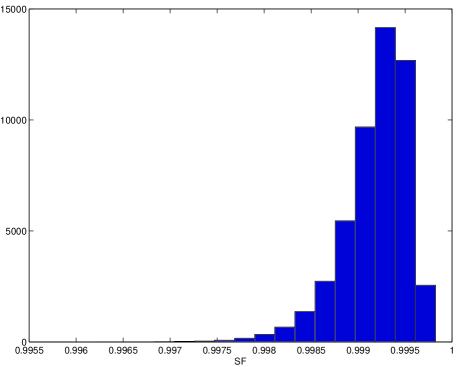
Figure 1: Distribution the Shapiro-Francia statistic obtained from 50000 independent Gaussian simulations of maps with 2164 pixels (independent pixel-to-pixel).

Given a sample of uncorrelated and normalized (zero mean, dispersion one) CMB data, the question we want to answer is “how well the data agree with the population of a Gaussian distribution $N(0,1)$” (the methods here used are also suited for testing a composite hypothesis where mean and dispersion are not specified).

Many goodness-of-fit methods have been developed to test normality (for a review see D’Agostino $\&$ Stephens 1986). Out of all we have chosen to apply the Shapiro-Francia one (Shapiro & Francia 1972), a modification of the Shapiro-Wilk test for large data sets. Implementation of the Shapiro-Francia requires the following steps: 1) - Estimation of the 1 dimensional array $\vec{c}$ corresponding to the expected sorted values obtained from independent Gaussian simulations $N(0,1)$. We define $\vec{b}=\vec{c}/||c||^{1/2}$ 2) - For a given sorted data set $\vec{x}$ , the Shapiro-Francia statistic $SF$ is defined as follows

$$SF={{(\sum_{i=1}^{N}b_{i}x_{i})^{2}}\over{N\sigma^{2}}},$$

where $N$ is the number of data and $\sigma$ is the dispersion. The expected value of this statistic for the Gaussian distribution is very close to one. Deviations from Gaussianity will result in values smaller than one. The distribution of the SF statistic for independent Gaussian realizations is presented in Figure 1.

Smooth goodness-of-fit methods have been constructed as powerful tests against distributions that might deviate “smoothly” from the normal $N(0,1)$ one. These methods are sensitive to the presence of skewness ($S$), kurtosis ($K$) and higher order moments. Some of them are defined based on orthonormal functions (Rayner $\&$ Best 1990) whereas others make use of powers of the distribution function (Thomas $\&$ Pierce 1979). The uncategorised smooth models proposed by Rayner $\&$ Best (1990) $S_{k}$ make use of the Hermite-Chebyshev polynomials $P_{n}$ and are defined by

$$S_{k}=\sum_{i=1}^{k}(\sum_{j=1}^{N}h_{i}(x_{j})/\sqrt{(}N))^{2},$$

where $h_{i}(x_{j})=P_{i}(x_{j})/\sqrt{(}n\!)$. The statistic $S_{k}$ is related to cumulants of order $\leq k$, such that for example:

$$S_{1}=N<x>^{2},~{}~{}~{}S_{2}=S_{1}+(N/2)(<x^{2}>-1)^{2},$$

$$S_{3}=S_{2}+(N/6)(<x^{3}>-3<x>)^{2},$$

$$S_{4}=S_{3}+(N/24)(<x^{4}>-6<x^{2}>+3)^{2},$$

where $<>$ denotes the average. And if $<x>=0$ and $<x^{2}>=1$, then $S_{3}=(N/6)S^{2}$ and $S_{4}=S_{3}+(N/24)K^{2}$. The $S_{k}$ statistic is distributed as a $\chi_{k}^{2}$ for the Gaussian case. We also make use in this paper of the smooth goodness-of-fit test $W_{k}$ proposed by Thomas $\&$ Pierce (1979) as a modification of Neyman’s one. This test is built on powers of the normal distribution function and compares sample means of these quantities with the expected values under the null hypothesis that the data correspond to a population sample of the normal distribution.

$$W_{k}=\sum_{i=1}^{k}\bigl{[}\sum_{j=1}^{i}a_{ij}u_{j}\bigr{]}^{2},k=1,2,3,4,...$$

$$u_{j}\equiv\frac{1}{N^{1/2}}{\sum}_{r=1}^{N}(y^{j}(x_{r})-\frac{1}{1+j})$$

where for the normal distribution $y(x_{r})\equiv erf(\frac{x_{r}-\mu}{\sigma})$, being $\mu,\sigma$ the mean and dispersion, and the coefficients $a_{ij}$ are given in Table 3 by Thomas & Pierce (1979) (e. g. $a_{11}=16.3172,a_{21}=-a_{22}=-27.3809$). Therefore, for $k=1,2$, for example, the statistics are

$$W_{1}=\frac{16.3172^{2}}{N}\bigl{[}{\sum}_{r=1}^{N}(y(x_{r})-\frac{1}{2})\bigr{]}^{2},$$

$$W_{2}=W_{1}+\frac{27.3809^{2}}{N}\bigl{[}{\sum}_{r=1}^{N}(y^{2}(x_{r})-\frac{1}{3}-y(x_{r})+\frac{1}{2})\bigr{]}^{2}.$$

These statistics, under the null hypothesis, are distributed as $\chi^{2}_{k}$. The distributions of values of the two smooth goodness-of-fit statistics for 50000 independent Gaussian realizations are presented in Figures 2 and 3. In both cases, and in the examples and applications presented below, the data are renormalized to zero mean and unit variance before the tests are applied. Because of that the $S_{k}$ statistics appear as $\chi_{k-2}^{2}$ distributions. The distributions of the two statistics converge to the expected ones. However one can see that the $W_{k}$ statistic converges faster to the expected distribution than the $S_{k}$.

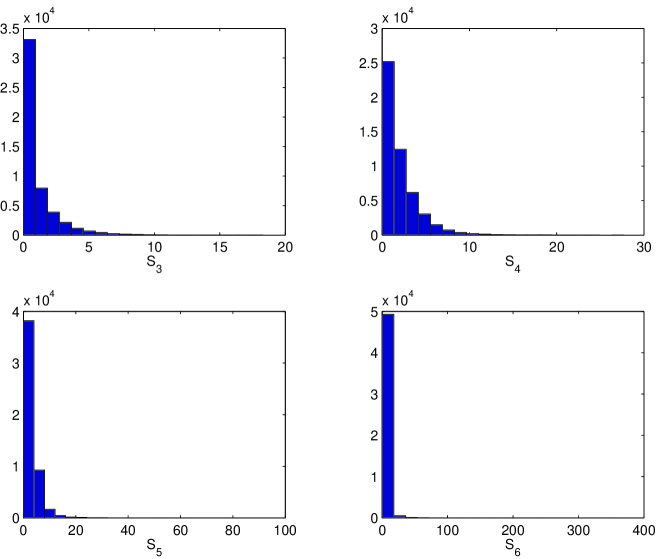
Figure 2: Distribution of $S_{k}$ smooth-goodness-of-fit statistics. From left to right, top to bottom $S_{k}$ corresponding to $S_{3},S_{4},S_{5},S_{6}$. Distributions obtained from 50000 independent Gaussian simulations of maps with 2164 pixels (pixel-to-pixel independent).

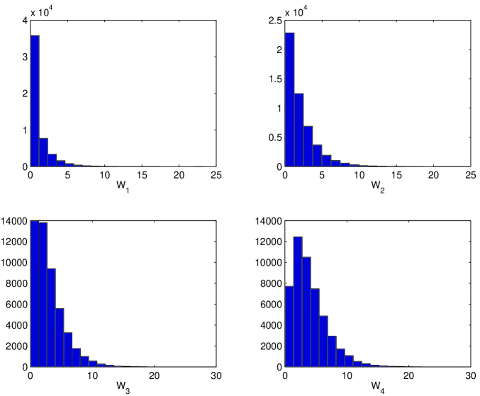
Figure 3: Distribution of $W_{k}$ smooth-goodness-of-fit statistics. From left to right, top to bottom $W_{k}$ corresponding to $W_{1},W_{2},W_{3},W_{4}$. Distributions obtained from 50000 independent Gaussian simulations of maps with 2164 pixels (pixel-to-pixel independent).

As an example of how well these methods work on separating Gaussian from nonGaussian data, we have applied them to simulated non Gaussian data following distributions as in Martínez-González et al. (2002). An array with 2164 independent pixels constitutes a simulation. The chosen number of pixels fits the number of central pixels in the MAXIMA map, later selected for analysis. The pixel value is drawn from a non Gaussian distribution obtained through the Edgeworth expansion characterised by a given skewness and kurtosis. Given an input skewness and kurtosis, the mean and dispersion value for these two statistics in the resulting simulations are given in Table 1, as well as the skewness and kurtosis power to discriminate between Gaussian and non Gaussian distributions. 10000 simulations were performed and the power of the Smooth Goodness of fit statistics presented in this paper is given for several input skewness and kurtosis values in Table 2 and Table 3. As one can see from these results, most of the presented goodness-of-fit statistics have more power than the directly calculated cumulants. The $W_{2}$ statistic is the one with higher discriminating power in most of the cases. Even so, the result is very dependent on the underlying distribution.

Table 1: Average and dispersion for the skewness and kurtosis values obtained from 10000 simulations drawn from Edgeworth expansions assuming skewness and kurtosis values denoted by $S\&K(input)$. The power of these two statistics is also given in columns 4 and 5.

S$\&$K(input)	Mean/Disp (S)	Mean/Disp (K)	Power(95/99$\%$) (S)	Power(95/99$\%$) (K)
0.0$\&$0.4	5.95e-4/0.0607	0.3170/0.1205	7.86/2.13	87.85/65.57
0.1$\&$0.0	0.0965/0.0503	-0.0342/0.0938	57.51/28.36	1.65/0.19
0.1$\&$0.3	0.0982/0.0581	0.2309/0.1157	57.49/32.25	67.26/37.05
0.1$\&$0.4	0.0968/0.0604	0.3180/0.1239	56.22/31.6	87.72/65.19
0.1$\&$0.5	0.0976/0.0624	0.4061/0.1273	56.46/32.67	97.08/86.75
0.1$\&$0.7	0.0976/0.0624	0.5820/0.1391	57.27/35.62	99.96/99.17
0.3$\&$0.3	0.2944/0.0565	0.2323/0.1320	99.96/99.86	64.90/38.87

Table 2: Power at $95\%$ and $99\%$ confidence level for the different statistics presented in this work (notation used for the table “$95\%/99\%$”). These results are based on 10000 Gaussian and non Gaussian simulations. The non Gaussian ones were obtained from the Edgeworth expansion for different values of skewness and kurtosis (skewness $S$ and kurtosis $K$ input values indicated in column 1).

S$\&$K	$S_{3}$	$S_{4}$	$S_{5}$	$S_{6}$	$W_{1}$	$W_{2}$	$W_{3}$	$W_{4}$
0.0$\&$0.4	8.95/2.46	74.04/53.18	66.48/36.26	71.98/23.32	6.80/1.67	83.03/64.75	77.20/58.76	74.38/52.97
0.1$\&$0.0	44.62/20.51	33.4/12.93	23.63/5.11	16.7/0.65	41.13/20.26	33.22/14.31	29.16/12.38	25.61/9.11
0.1$\&$0.3	46.52/25.03	68.46/47.10	62.03/31.30	61.27/15.97	45.99/25.31	74.22/53.98	68.43/48.04	65.38/42.2
0.1$\&$0.4	45.58/24.99	84.35/67.6	79.38/52.71	81.91/35.99	46.35/25.42	90.79/77.35	87.24/72.32	84.81/66.26
0.1$\&$0.5	46.35/26.03	94.56/86.13	92.80/74.72	95.00/62.99	47.64/27.23	98.27/93.92	97.04/91.54	96.23/88.04
0.1$\&$0.7	47.96/28.82	99.75/98.92	99.56/97.05	99.91/97.06	50.88/31.07	99.99/99.95	99.97/99.89	99.96/99.75
0.3$\&$0.3	99.95/99.75	99.90/99.51	99.86/99.58	99.80/92.81	99.96/99.85	99.95/99.72	99.92/99.46	99.88/99.00

Table 3: Power at $95\%$ and $99\%$ confidence level for the Shapiro-Francia statistic (notation used for the table “$95\%/99\%$”). These results are based on 10000 Gaussian and non Gaussian simulations. The non Gaussian ones were obtained from the Edgeworth expansion for different values of skewness and kurtosis (skewness $S$ and kurtosis $K$ input values indicated in column 1).

S$\&$K	SF
0.0$\&$0.4	70.82/47.30
0.1$\&$0.0	30.97/13.69
0.1$\&$0.3	65.21/42.45
0.1$\&$0.4	83.37/64.62
0.1$\&$0.5	95.35/86.27
0.1$\&$0.7	99.90/99.56
0.3$\&$0.3	99.94/99.66

The cases simulated above are based on an Edgeworth expansion considering all cumulants of order greater than 2 equal to zero, except for those of order 3 and 4. The smooth goodness of fit statistics combine information from cumulants of any order and in particular of orders below 7. We have performed simulations based on the Edgeworth expansion including non null cumulants up to order 6. The simulated maps do not preserve the input cumulant values. Mean and dispersion values of the cumulants calculated out of 10000 simulations are presented in Table 4. The power of the cumulants to differentiate between a Gaussian and another distribution (based on the Edgeworth expansion) is given at the $95\%$ in Table 5.

Table 4: Average and dispersion for the skewness, kurtosis, 5th and 6th order cumulants obtained from 10000 simulations drawn from Edgeworth expansions assuming skewness, kurtosis, 5th and 6th order cumulant values denoted by $S\&K\&k5\&k6(input)$.

S$\&$K$\&$k5$\&$k6 (input)	Mean/Disp (S)	Mean/Disp (K)	Mean/Disp (k5)	Mean/Disp (k6)
0.1$\&$0.4$\&$1.0$\&$3.0	0.0955/0.0673	0.3169/0.1540	0.8156/0.3246	1.3604/0.67157
0.1$\&$0.3$\&$1.0$\&$3.0	0.1264/0.0617	0.1475/0.1421	1.0634/0.2610	1.2203/0.5402
0.1$\&$0.4$\&$0.8$\&$3.0	0.0937/0.0677	0.3160/0.1563	0.6076/0.3450	1.4349/0.6925
0.1$\&$0.3$\&$0.8$\&$3.0	0.1397/0.0602	0.1123/0.1417	0.9523/0.2714	1.2030/0.5468

Table 5: Power of the skewness, kurtosis, 5th and 6th order cumulants at the $95\%$ confidence level. Results drawn from 10000 simulations based on Edgeworth expansions assuming skewness, kurtosis, 5th and 6th order cumulant values denoted by $S\&K\&k5\&k6(input)$.

S$\&$K$\&$k5$\&$k6 (input)	Power (S)	Power (K)	Power (k5)	Power (k6)
0.1$\&$0.4$\&$1.0$\&$3.0	54.91	81.48	91.09	73.10
0.1$\&$0.3$\&$1.0$\&$3.0	73.52	41.46	99.72	69.97
0.1$\&$0.4$\&$0.8$\&$3.0	53.94	81.27	75.17	76.32
0.1$\&$0.3$\&$0.8$\&$3.0	80.72	32.17	98.86	68.17

The smooth goodness of fit statistics as well as the Shapiro-Francia test have been calculated for the simulated maps including cumulants up to order 6. Powers at the $95\%$ confidence level are presented in Table 6. As one can see in all cases the Shapiro-Francia test is the most powerful of all the implemented tests. It is difficult to asses whether some tests will be more convenient than others when trying to detect non Gaussianity. Moreover, as pointed out by Bromley & Tegmark (1999) even if non Gaussianity is detected by one statistical method, the confidence level has to be established taking into account all the methods applied.

Table 6: Power at $95\%$ confidence level for the different statistics presented in this work. These results are based on 10000 Gaussian and non Gaussian simulations. The non Gaussian ones were obtained from the Edgeworth expansion for different values of skewness, kurtosis, 5th and 6th order cumulants (input values for skew $S$, kurt $K$, 5th $k5$ and 6th $k6$ order cumulants indicated in column 1.

S$\&$K$\&$k5$\&$k6	$S_{3}$	$S_{4}$	$S_{5}$	$S_{6}$	$W_{1}$	$W_{2}$	$W_{3}$	$W_{4}$	SF
0.1$\&$0.4$\&$1.0$\&$3.0	45.92	78.11	93.63	97.54	9.61	17.04	37.68	61.16	99.91
0.1$\&$0.3$\&$1.0$\&$3.0	64.77	60.28	98.87	98.98	13.30	14.18	37.29	41.48	99.98
0.1$\&$0.4$\&$0.8$\&$3.0	44.85	78.46	87.77	94.78	12.96	20.30	35.95	52.81	99.36
0.1$\&$0.3$\&$0.8$\&$3.0	72.82	64.30	97.58	97.54	22.13	21.61	46.99	44.46	99.88

3 MAXIMA data analysis. Results

The goodness-of-fit tests previously described are optimal for testing univariate Gaussian distributions. We therefore first of all transform the MAXIMA data by multiplying it by the inverse of the Cholesky matrix corresponding to signal plus noise. We first calculate the Cholesky decomposition corresponding to the “data correlation matrix”. To do that a cosmological model fitting the data has been assumed. MAXIMA data is better fitted to a cosmological model characterised by $\omega_{b}=0.105$, $\omega_{c}=0.595$, $\omega_{\Lambda}=0.3$ and $h=0.53$ (Balbi et al. 2000). Simulations of this model are used to calculate the signal correlation matrix. The so called “data correlation matrix” is the sum of the signal and noise correlation matrices.

Once the data respond to independent values drawn from a normal distribution with mean zero and dispersion one $N(0,1)$, we calculate the above introduced smooth goodness-of-fit statistics as well as the Shapiro-Francia one. Noise levels are specially high at some pixels resulting in large correlation values off the diagonal. Most of these pixels appear to be in the border of the observed region. To make sure the previous test is not dominated by noise we have selected pixels in the central area of the one covered by MAXIMA observations. We select pixels with right ascention in the range $226.47-238.24$ degs and declination ranging from $55.567$ degs to $61.7$ degs. These pixels amount to a total of 2164. In order to see if the MAXIMA data are compatible with Gaussianity we have simulated 50000 maps with 2164 pixels independently generated from a $N(0,1)$ distribution. The statistic values obtained from the data as well as the probability of having Gaussian values larger than the MAXIMA ones are presented in Table 7. One should keep in mind that in the case of the Shapiro-Francia test, this is a confidence level taken from the left. As one can see, the MAXIMA data are compatible with Gaussianity.

Table 7: Statistic values obtained for the MAXIMA data and probability of being drawn from a Gaussian distribution (Prob $>=MAXIMA$) from independent Gaussian simulations

statistic	data value	Prob$\%$
S	0.035	25.23
K	0.058	28.04
k5	-0.276	89.43
k6	-0.068	48.32
$S_{3}$	0.446	50.29
$S_{4}$	0.717	69.74
$S_{5}$	2.091	52.34
$S_{6}$	2.101	64.37
$W_{1}$	0.948	33.23
$W_{2}$	1.050	59.64
$W_{3}$	1.170	76.29
$W_{4}$	1.177	88.40
SF	0.9994	30.06

The process we follow to decorrelate the observations could be thought to introduce some artifacts that could make the comparison with independent $N(0,1)$ simulations not appropiate. To answer this question we simulate data taking into account MAXIMA observational constraints as well as the noise information. Afterwards these simulations are decorrelated following the same steps as in the the real data case. The statistical tests are applied on these decorrelated simulations and compared with the results obtained from the decorrelated MAXIMA data.

As a first step we “tried” simulating CMB skies as those seen by MAXIMA. Those simulations included signal plus noise. The quoted word refers to the signal simulations. To simplify the simulation process we have based the simulations on the HEALpix pixelization (Gorski, Hivon & Wandelt 1999). This does not exactly reproduce the observational grid but we consider the approach good enough for the proposed test. These maps are simulated following these steps: 1) The $a_{lm}$ coefficients are generated assuming the power spectrum corresponding to the cosmological model that best fit the MAXIMA data (Balbi et al. 2000) multiplied by the beam pattern. 2) We use the HEALpix subroutines to generate a map with the obtained $a_{lm}$s. The maximum $l$ corresponds to a $nside=512$, that is, the generated pixels are $7\times 7$ arcmin². MAXIMA pixels are $8\times 8$ arcmin². Moreover, the MAXIMA pixelization does not agree with the HEALpix pixelization. The simulated pixel values are assigned to MAXIMA pixels based on their right ascention and declination. Since the processing time is quite long we only performed 300 simulations. Noise simulations are obtained by multiplying a pixel-to-pixel independently generated (from a Gaussian distribution $N(0,1)$) map by the Cholesky matrix corresponding to the noise correlation matrix.

The simulated maps are afterwards multiplied by the inverse of the Cholesky matrix as it is done with the data. Results for the different statistics evaluated on the MAXIMA data and probability of these values to be drawn from a Gaussian distribution are presented in Table 8. The MAXIMA values are in agreement with Gaussian ones as was obtained in the previous case. The probability values obtained for the different statistics in Tables 7 and 8 are of the same order. One can however notice a larger difference in the case of the $K$ statistic. We have checked the $K$ values obtained in both cases (for Tables 7 and 8). We have done the exercise of obtaining the distribution of $|K|$ values directly from the $K$ ones (case 1) and combining the $S_{3}$ and $S_{4}$ values as indicated in section 2 (case 2). In case 1, the MAXIMA value is $|K_{MAXIMA}|=0.058$ (as indicated in Table 7) and the probability of getting values greater or equal than this one is $58.15\%$ for simulations in Table 7 and $65.00\%$ for simulations in Table 8. In case 2, the MAXIMA value is $|K_{MAXIMA}|=0.055$ and the probability of getting values greater or equal than this one is $60.18\%$ for simulations in Table 7 and $65.00\%$ for simulations in Table 8. There is therefore compatibility between these two cases. Moreover, the distribution of the absolute value of the $K$ statistic seems not to change much between simulations in Table 7 and those in Table 8. What might be happening is that the distribution of $K$ values converges slowly and therefore 300 simulations, in the case of those in Table 8, might not be enough to asses a precise probability value. Nevertheless this result does not affect our final conclusion, that the MAXIMA data are found to be compatible with Gaussianity under the Goodness-of-fit tests applied in this work.

Finally, we would like to note the importance of decorrelating the data in order to asses its departure from Gaussianity, by looking at the Goodness-of-fit statistics introduced in this paper. As already mentioned, these are statistics designed to test univariate Gaussianity. Applying these methods to correlated data will only have partial meaning and their power will be diluted. We should however mention the fact that the decorrelation procedure will modify the distribution of the data we are analysing. It is difficult to quantify this effect as it would depend on the deviations from Gaussianity present in the analysed data as well as on the corresponding Cholesky matrix. Just as an example we have applied all the statistical tests discussed in this work to two cases in which a certain amount of non-Gaussianity is introduced in correlated simulations. The results are presented in Table 9. The power of the statistics in distinguishing Gaussian from non-Gaussian simulations is shown in columns 3 and 4 for the two cases considered. In each column, the first number represents the power at the $95\%$ c.l. when looking at correlated simulations. The second number indicates the power at the $95\%$ c.l. after decorrelating the simulations (the inverse of the Cholesky matrix corresponding to MAXIMA data is used for this). The Gaussian simulations are done as explained in the fourth paragraph of this Section, following MAXIMA’s constraints. Each of the non-Gaussian ones consists of the sum of a Gaussian simulation plus a non-Gaussian one with the same correlation (the fact that we have a sum of two simulations with the same correlation is taken into account when decorrelating). The non-Gaussian simulations are generated based on an Edgeworth expansion as the ones in Section 2, afterwards multiplied by the Cholesky matrix corresponding to the MAXIMA data. As can be seeing from the Table, any of the suggested methods have a larger power after decorrelating, even if then distributions have been modified in the process.

Table 8: Probability of the MAXIMA data of being drawn from a Gaussian distribution ( Prob $>=MAXIMA$). Simulations consist of the sum of signal plus noise following the MAXIMA observational constraints. Both the data and the simulations are decorrelated (as explained in the text) before they are analysed.

statistic	Prob$\%$
S	27.67
K	48.33
k5	84.33
k6	46.33
$S_{3}$	51.33
$S_{4}$	73.00
$S_{5}$	57.67
$S_{6}$	68.33
$W_{1}$	34.00
$W_{2}$	63.67
$W_{3}$	76.67
$W_{4}$	89.00
SF	27.00

Table 9: Power of the different statistical tests to distinguish Gaussian from non-Gaussian simulations before and after decorrelating (bef/aft). For the two cases considered, the non-Gaussian simulations are generated as explained in the text and based on Edgeworth expansions with $S=0.5,K=0.5$ (column 2) and $S=0.7,K=0.7$ (column 3).

statistic	Power($95\%$) bef/aft $S=0.5,K=0.5$	Power($95\%$) bef/aft $S=0.7,K=0.7$
S	20.66/86.33	19.66/99.00
K	26.00/6.66	23.33/11.66
k5	18.33/8.66	14.33/8.33
k6	25.33/6.00	22.66/4.66
$S_{3}$	19.99/76.00	23.00/96.00
$S_{4}$	28.66/53.00	24.66/84.67
$S_{5}$	26.66/28.33	23.00/62.00
$S_{6}$	26.00/18.33	23.66/41.33
$W_{1}$	13.66/78.00	14.99/98.33
$W_{2}$	18.00/66.33	19.66/93.33
$W_{3}$	17.66/69.00	19.66/92.66
$W_{4}$	22.66/63.00	21.66/91.33
SF	24.00/49.00	20.33/85.66

4 Discussion and Conclusions

The future detection of non Gaussianity in CMB data will rely on the power of the applied statistical methods. At present, it is not an easy task to establish which methods will be more powerful. Physically motivated deviations from Gaussianity generated in theories alternative to the Standard Inflationary one are still not well characterised. It is however needed to know which methods could be better suited to detect certain types of non Gaussianity even if they are tested on toy model simulations.

We have implemented goodness-of-fit statistics developed to detect deviations from a given distribution, in our case from the Gaussian one. Three different methods have been tested against simulations including deviations from the Gaussian distribution. The selected methods were developed by Shapiro & Francia (1972), Thomas & Pierce (1979) and Rayner & Best (1990). The last two ones belong to the so called smooth goodness-of-fit tests. The performance of these methods was checked on simulations based on the Edgeworth expansion including distortions produced by the presence of cumulants of order higher than two. A strong conclusion can not be drawn from this exercise. If only skewness and kurtosis are present, the statistic $W_{2}$ developed by Thomas & Pierce (1979) has more power than the rest of applied statistics. The presence of cumulants of order 5 and 6 seems to be better detected by the Shapiro-Francia test.

Several statistical methods have already been applied to the MAXIMA data in the search for non Gaussianity. Wu et al. (2001) calculated moments, cumulants, Minkowski functionals, Kolmogorov and $\chi^{2}$ tests of the real and Wiener filtered data as well as of the eigenmodes and signal-whitened data. Santos et al. (2002) obtained the bispectrum value for these data. In both cases comparison with Gaussian predictions confirmed the compatibility of the MAXIMA data with Gaussianity. We have added three more tests to the ones applied to MAXIMA (also see Aliaga et al. (2003) where constraints on $S$ snd $K$ are impossed based on that data). The tests are optimal in the case of non-correlated data. Moreover, they can be applied even in cases in which the observations are not taken on a regular grid. As a first step in our method we have decorrelated the observations by multiplying by the inverse of the corresponding Cholesky matrix. This is feasible in this case in which only a region of the whole sky was covered as any matrix operation is computationally very expensive. Future application of these methods could in any case be done by decorrelating data region by region of the sky. For the case analysed in this work, one can conclude that the MAXIMA data are compatible with Gaussianity under the three goodness-of-fit methods applied.

References

- [1] Acquaviva, V., Bartolo, N., Matarrese, S. & Riotto, A. 2002, astro-ph/0209156
- [2] Aliaga, A.M., Martínez-González, E., Cayón, L., Argüeso, F., Sanz, J.L. & Barreiro, R.B. 2003, submitted to New Astronomy Reviews
- [3] Balbi, A. et al. 2000, ApJ, 545, L1
- [4] Bernardeau, F. & Uzan, J-P. 2002, Physical Review D, 66, 103506
- [5] Bromley, B.C. & Tegmark, M. 1999, ApJ, 524, L79
- [6] Cayón, L., Martínez-González, E., Argüeso, F., Banday, A.J. & Gorski, K.M. 2003, MNRAS, 339, 1189
- [7] D’Agostino, R.B. & Stephens, M.A. 1986, “Goodness-of-fit techniques”, Marcel Dekker, INC. New York
- [8] Durrer, R. 1999, New Astronomy Reviews, 43, 111
- [9] Gangui, A., Lucchin, F., Matarrese, S. & Mollerach, S. 1994, ApJ, 430, 447
- [10] Gorski, K.M., Hivon, E. & Wandelt, B.D. 1999, “Evolution of Large Scale Structure: from Recombination to Garching”, ed. A.J. Banday, R.K. Seth & L.N. da Costa, astro-ph/9812350
- [11] Gupta, S., Berera, A., Heavens, A.F. & Matarresse, S. 2002, Physical Review D, 66, 043510
- [12] Hanany, S. et al. 2000, ApJ, 545, L5
- [13] Komatsu, E. & Spergel, D.N. 2001, Physical Review D, 63, 063002
- [14] Komatsu, E., Wandelt, B.D., Spergel, D.N., Banday, A.J. & Gorski, K.M. 2002, ApJ, 566, 19
- [15] Landriau, M. & Shellard, E.P.S. 2002, astro-ph/0208540
- [16] Martínez-González, E., Gallegos, J.E., Argüeso, F., Cayón, L. & Sanz, J.L. 2002, MNRAS, 336, 22
- [17] Peebles,P.J.E., 1999a, ApJ,510,523
- [18] Peebles,P.J.E., 1999b, ApJ,510,531
- [19] Rayner, J.C.W. & Best, D.J. 1990, International Statistical Review, 58, 9
- [20] Santos, M.G. et al. 2002a, Physical Review Letters, 88, 241302
- [21] Santos, M.G. et al. 2002b, astro-ph/0211123
- [22] Shapiro, S.S. & Francia, R.S. 1972, Journal of American Statistical Association, 67, 215
- [23] Thomas, D.R.& Pierce, D.A. 1979, Journal of the American Statistical Association, 74, 441
- [24] Wu, J.H.P. et al. 2001, Physical Review Letters, 87, 251303