Linear Polarization Observations of Water Masers in W3 IRS 5

Abstract

We present a magnetic field mapping of water maser clouds in the star-forming region W3 IRS 5, which has been made on the basis of the linear polarization VLBI observation. Using the Very Long Baseline Array (VLBA) at 22.2 GHz, 16 of 61 detected water masers were found to be linearly polarized with polarization degrees up to 13 %. Although 10 polarized features were widely distributed in the whole W3 IRS 5 water maser region, they had similar position angles of the magnetic field vectors ($\sim$ 75^∘ from the north). The magnetic field vectors are roughly perpendicular to the spatial alignments of the maser features. They are consistent with the hourglass model of the magnetic field, which was previously proposed to explain the magnetic field in the whole W3 Main region ($r\sim$ 0.1 pc). They are, on the other hand, not aligned to the directions of maser feature proper motions observed previously. This implies that the W3 IRS 5 magnetic field was controlled by a collapse of the W3 Main molecular cloud rather than the outflow originated from W3 IRS 5.

1 Introduction

Birth of massive stars is characterized by a collapse of molecular cloud core when self-gravity overwhelms the magnetic pressure in the core as a result of magnetic field dilution. In this situation, the core is not supported by the magnetic field pressure in the cloud core any more, and called to be magnetically super-critical (e.g., Shu, Adams, & Lizano 1987; Feigelson & Montmerle 1999, and references therein). Measurements of the magnetic field strengths and directions in star-forming regions have been made in a variety of spatial scales, from whole star-forming regions (1–10 pc) down to individual molecular cloud cores (e.g., Heiles et al. 1993; McKee et al. 1993; Evans II 1999, and references therein). In the smaller scale, the measurements were made mainly with radio interferometers with higher angular resolution. However, because of complicated structures of the magnetic fields expected from the presence of the dense clumps and outflows, and because of the uncertainty in calibration in the polarimetric interferometry, it is more difficult to map the magnetic field accurately in this scale.

Water maser emission is often associated with star-forming regions (SFRs) with energetic outflows from young stellar objects (YSOs) (e.g., Elitzur 1992a, b and references therein). VLBI observations have revealed that water maser emission consists of clusters of compact maser features with a typical size of 1 AU and a velocity width of 1 km s^-1(e.g., Reid & Moran 1981). Measurements of Doppler velocities and proper motions of maser features have led to the conclusion that the spatial motions of maser features really reflect the true three-dimensional gas kinematics (e.g., Gwinn, Moran, & Reid 1992; Torrelles et al. 2001a, b). Previous observations have found expansion motions produced by outflows from YSOs or expanding HII regions (e.g., Imai  et al. 2000, hereafter Paper I, and references therein). Shocks, which have velocities exceeding about 20 km s^-1 and are running into high-density ($n_{\mbox{\tiny H${}_{2}$}}\>\geq$ 3$\times$10⁶ cm^-3) magnetized material, successfully explain the water maser emission associated with energetic YSO outflows (e.g., Hollenbach & McKee 1989; Elitzur, Hollenbach, & McKee 1989, 1992; Hollenbach, Elitzur, & McKee 1993).

Polarimetric mapping of individual water maser features were made for the first time using VLBI data in W51 M by Leppänen, Liljeström, & Diamond (1998) (hereafter LLD). They found that the observed directions of linear polarization were well aligned along a stream of water maser features found in W51 M. It should be noted that the observed direction of the linear polarization does not straightly indicate the magnetic field direction of the cloud because it depends on the angle between the magnetic field and the photon propagation direction (toward an observer) (e.g., Goldreich, Keeley, & Kwan 1973; Deguchi & Watson 1986b, 1990). In the case of W51 M, the observed directions of linear polarization were interpreted to be parallel to the magnetic field vector projected on the sky plane because the field vector is expected to be roughly tangential to the line of sight due to coupling with the Sagittarius spiral arm. LLD concluded that the alignment of the water maser linear polarization was created by shocks caused by the nearby expanding HII region. The linear polarization of water masers as a tracer of the interstellar magnetic fields is indirectly supported by that the linear polarization directions in a maser region are stable on a timescale of several years despite of much shorter time scale of lifetimes and flux variability of maser features (Abraham & Vilas Boas 1994; LLD; Horiuchi, Migenes, & Deguchi 2000; Horiuchi & Kameya 2000; Horiuchi & Kemaya 2003 in preparation).

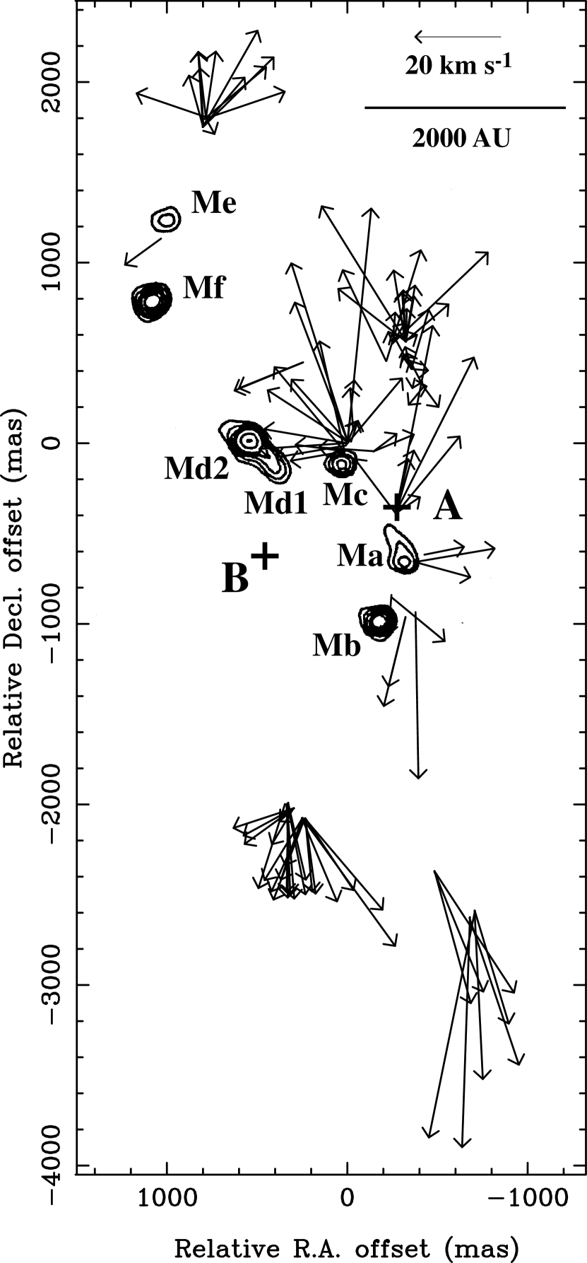
Figure 1: Water maser features and compact radio continuum sources in W3 IRS 5. Arrows indicate locations and proper motions of maser features, which were revealed by Paper I. The arrow length indicates the magnitude of the proper motion per year ($\times$325), respectively. The radio continuum sources, which were mapped by Claussen et al. (1994), are shown as contours. The designations the continuum sources are same as those in Tieftrunk et al. (1997). Two plus marks A and B indicate the locations of driving sources of the outflows in W3 IRS 5, which were estimated by Paper I.

This paper discusses the results of magnetic field mapping of water maser clouds in the massive-star forming region W3 IRS 5 revealed by a VLBI observation. W3 IRS 5 is considered to be at the very early phase of star formation because of lack of high velocity components in the water masers, as suggested by Genzel & Downes (1977). Previous observations also supported this interpretation on W3 IRS 5 (e.g., Claussen et al. 1994; Tieftrunk et al. 1997; Roberts, Crutcher, & Troland 1997). In a 2″$\times$3″ field of W3 IRS 5, Claussen et al. (1994) and Tieftrunk et al. (1997) found the distribution of a cluster of centimeter-continuum emission sources. Imai  et al. (2000) investigated the 3-D kinematics of the water masers in W3 IRS 5 and estimated a distance to this region to be 1.83$\pm$0.14 kpc. In the present paper, the value of 1.8 kpc is adopted as the distance to W3 IRS 5. Imai, Deguchi, & Sasao (2002) (hereafter Paper II) investigated the physical condition of the region where the water masers are excited. They found that turbulent motions dominate the morphology and kinematics on a microscopic scale (down to 0.01 AU). Figure 1 shows the distribution and proper motions of the water maser features found in Paper I.

Troland et al. (1989) and Roberts et al. (1993) (hereafter RCTG) measured the Zeeman effect of the HI line in W3 IRS 5. They revealed the magnetic field projected in the line of sight on a scale of $\sim$ 0.6 pc, and demonstrated an ”hourglass” model of the magnetic field. The above scale is roughly equivalent to the core size found in this cloud found in the ¹³CO line by Hayashi, Kobayashi, & Hasegawa (1989). A pinch of the hourglass was found to be located very close to W3 IRS 5 region and to have the magnetic field strength higher than 1 mG. Greaves, Murray, & Holland (1994) also made a polarimetric observation at sub-millimeter wavelengths and estimated the magnetic field in W3 IRS 5 on a scale of 0.1 pc; the result supports the hourglass model. Barvainis & Deguchi (1989) found that the W3 IRS 5 water masers were highly linearly polarized. Sarma, Troland, & Romney (2001) (hereafter STR) and Sarma et al. (2002) (hereafter STCR) measured the Zeeman effect of the bright components of the water masers and estimated the magnetic field strength along the line of sight to be $\sim$ 30 mG.

In the present paper, we focus on an issue whether or not the magnetic field measured in water masers traces that found on the larger scale. The cause that determines the shape of the large-scale magnetic field is also speculated: either the collapse of the parent molecular cloud or the formation of a magneto-hydrodynamical jet. Section 2 describes the polarimetic observations using the Very Long Baseline Array (VLBA) and the Very Large Array (VLA) of the National Radio Astronomy Observatory (NRAO) and data reduction. The results are presented in §3. Section 4 discusses mainly the relation between the measured directions of maser linear polarization and possible directions and strength of the magnetic field in the observed scale ($<$5″) of W3 IRS 5.

2 Observations and data reduction

The polarimetric observation of water masers in W3 IRS 5 was made on 1998 November 21 using 10 telescopes of the VLBA. The water masers and calibrators (NRAO 150, JVAS 0212$+$735, and 0423$-$014) were observed for 10 hrs in total. The observed signals were recorded in a 4-MHz base band with both right and left circular polarization (RCP, LCP) in 2-bit sampling. The recorded data were correlated with the VLBA correlator in Socorro, which yielded parallel and cross-hand visibilities with 128 spectral channels. The correlated data covered a velocity range of $-$58 km s^-1 $\leq$ $V_{\mbox{\scriptsize LSR}}$$\leq$ $-$5 km s^-1 and a velocity spacing of 0.42 km s^-1 per spectral channel.

Data calibration and imaging were made using the procedures in AIPS mostly. First, the data of the parallel-hand-polarization visibilities were reduced in the usual procedures (e.g., Reid 1995; Diamond 1995) and fringe-fitting, self-calibration, and complex bandpass solutions were obtained independently in RCP and LCP. Although the water maser emission was strong enough to apply the ”template method” to calibrate the visibility amplitudes (Diamond, 1995), the band width of 4 MHz was too narrow to obtain a sufficient number of emission-free velocity channels in the template total-power spectrum of the maser emission. Instead, we applied tables of the measured system noise temperatures and antenna gains. In the self-calibration, we obtained a Stokes I  maser map of the velocity component (maser spot) at $-$40.2 km s^-1 and complex gain solutions in every 6 s.

Second, the instrumental polarization parameters (D-terms) of the telescopes were obtained using the AIPS RUN script CROSSPOL and the task LPCAL with scans of 0420$-$014, which is well linearly polarized. The D-term solutions were applied to the maser data. After the D-term calibration, the Stokes I, Q, U maps of maser spots were obtained independently. The naturally-weighted synthesized beam was 0.68$\times$0.49 mas, with the major axis at a position angle (PA) $PA\>=$ 3^∘.3. No smoothing in velocity channel was applied. The detection limit of about 30 mJy beam^-1 at a 5-$\sigma$ noise was obtained in velocity channels without bright maser emission. Before making the final image cubes, we looked for the masers by making wider maps covering a 2″$\times$5″ field with a larger synthesized beam.

Third, each velocity component (maser spot, see e.g., Gwinn 1994a, b; Paper II) in the image cube was fitted by a two-dimensional Gaussian brightness distribution using the AIPS task JMFIT. The uncertainty of the estimated position due to thermal noise was 3 microarcseconds ($\mu$as) for a 1-Jy spot. On the other hand, positional accuracy of the brightness peak of a maser feature (a cluster of maser spots) depends on the distribution of maser spots in the feature and the brightness distributions of the maser spots and limited to be typically 10 $\mu$as. The electric vector position angle (EVPA, see LLD), EVPA $=$ arctan($Q/U$)/2 of each maser spot was calculated from the Stokes $Q$ and $U$ parameters. For each maser feature (a cluster of maser spots existing together within   1 mas and   1 km s^-1 in position and velocity, Paper I and II), the degree of linear polarization and the EVPA were obtained from the Stokes parameters (I, Q, U) of the intensity peak in the maser feature.

The water masers were also observed with the VLA (26 antennas) in C-configuration on 1998 November 28, one week later the VLBA observation. The water masers and calibrators (3C 48, 0420$-$014, and 3C 138) were scanned for 2 hrs in total. The observed signals were recorded in a 3-MHz base band both in right and left circular polarization. The correlated data had 64 spectral channels with a velocity spacing of 0.63 km s^-1 per spectral channel. The D-terms of the antennas were obtained from the scans of 3C 48, which covered a variation of parallactic angle over 180^∘, assuming the intrinsic EVPA of $-$72^∘.5. Then we confirmed that the obtained EVPAs of 3C 138 and 0420$-$024 were consistent with those previously obtained by Akujor et al. (1993) and Marscher et al. (2002), respectively.

The EVPA at $V_{\mbox{\scriptsize LSR}}$$=$ $-$42.2 km s^-1 in the maser feature W3 IRS 5:I2003 5 (see table 1) was compared between the VLBA and VLBA data. At this velocity, the maser spot was most prominent and its polarimetric parameters were well determined. A correction ($\Delta$EVPA $=$ 39.^∘3) was applied to the EVPAs obtained with the VLBA. Taking into account the variation of EVPA in the maser feature ($\leq$ 3^∘), the ambiguity of the assumed EVPA of 3C 48 ($\sim$ 5^∘), and the accuracy of the calibration of the VLA data (uncertainty in R$-$L phase determination, $\leq$ 0.3^∘), the accuracy of EVPA was expected to be $\sim$6^∘. Because the VLA observation was made 7 days after the VLBA observation, the estimated EVPAs might suffer from the EVPA time variation of the feature W3 IRS 5:I2003 5.

3 Results

We detected 61 maser features consisting of 290 maser spots. These numbers are smaller by factors of 2–3 and 4–7, respectively, than those in the previous VLBA observations (Paper I, see also Paper II) while the sensitivity of the present observation was better than the previous ones. The decrease of features was likely due to less activity in maser excitation, while the decrease of spots was due to less velocity resolution by a factor of 4 in the present observation.

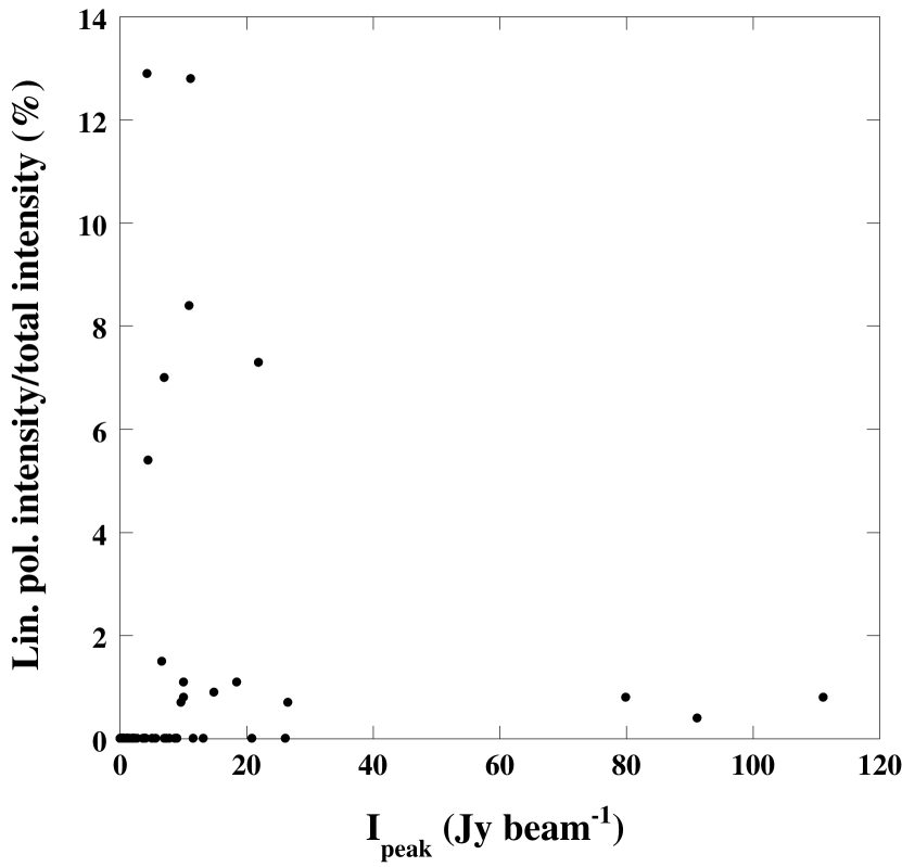
Figure 2: Distribution of polarization degrees of maser features against their peak intensities.

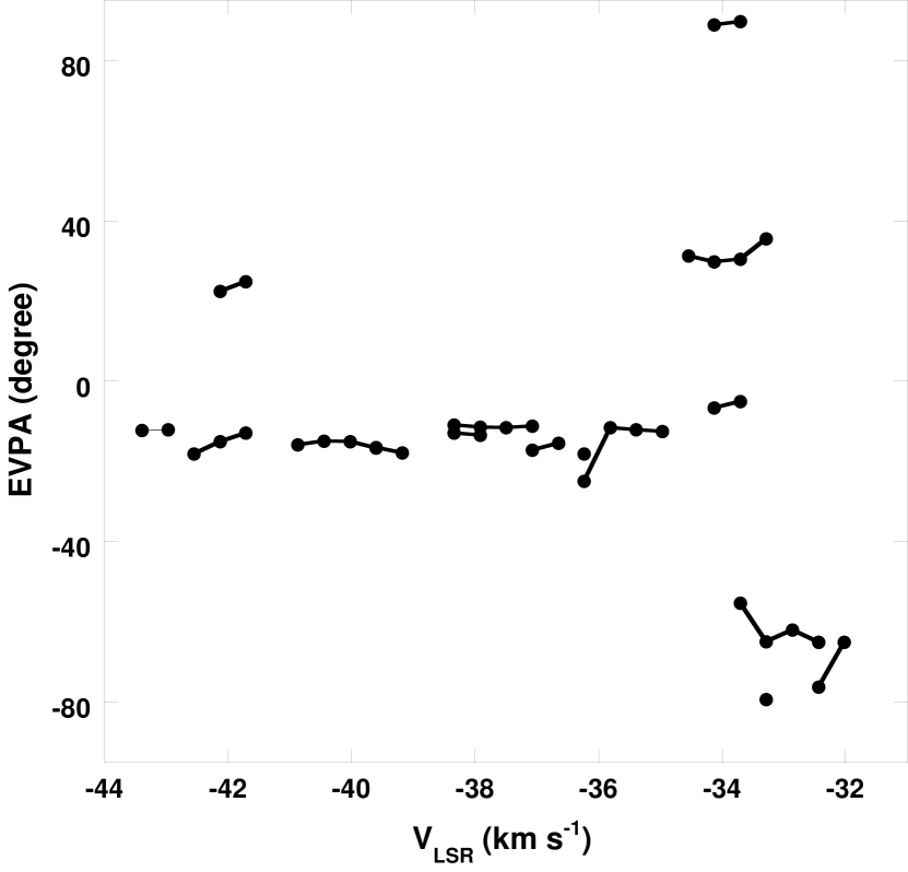
Figure 3: Distribution of EVPAs of maser spots against their Doppler velocities. A filled circle shows the maser spot detected its linear polarization. Maser spots in the same maser feature are connected each other with a thick line.

Table 1 summarizes the parameters of water maser features in W3 IRS 5. Only for 15 of 61 features, the proper motions were measured previously in Paper I. It was difficult to identify the same features between the observations of Paper I and the present work because many features were likely to appear and disappear in the crowded regions during the epoch separation of 11 month. The highest degrees of polarization was 13% in the present observation, which was smaller than those (up to 30%) found in a previous single dish observation (Barvainis & Deguchi, 1989) and an unpublished VLBI observation with a 400-km baseline. As shown in figure 2, no correlation was found between a feature intensity and a degree of linear polarization. LLD found a systematic change of EVPAs in a single maser feature with the full velocity width $\Delta V\>=$ 1.3 km s^-1. On the other hand, as shown in figure 3, EVPAs were almost the same (within 15^∘) in all of the features with measured linear polarization in W3 IRS 5.

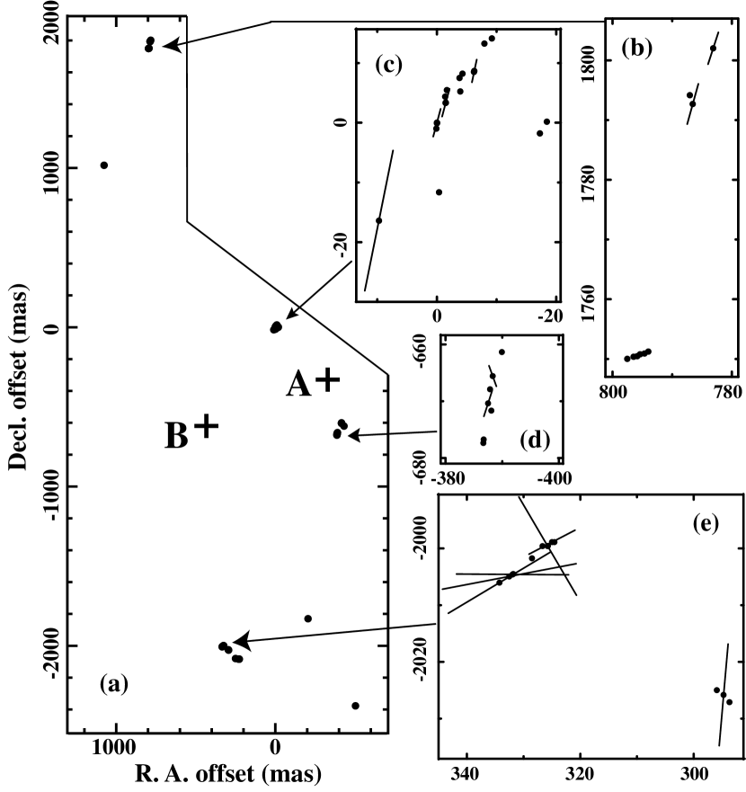
Figure 4: Map of linearly-polarized maser features in W3 IRS 5. (a): Locations of the maser features (filled circle) detected on 1998 November 21. Two plus marks are the same as those in figure 1. The locations of the maser features were estimated with respect to the driving sources of the outflows by assuming the stable distribution of clusters of maser features among observations made in the previous (Paper I) and the present works. The location uncertainty of the A outflow will be within 100 mas. (b)-(e): Details of the feature distribution and the directions of linear polarization of the features. A length and a position angle of a bar indicate a logarithmic scale of the degree of linear polarization and an EVPA, respectively.

Figure 4 presents the spatial distribution and the linear polarization directions of the maser features. The present maser map was easily overlaid on the previous ones in Paper I. We found that a cluster of maser features is elongated in the north–west and south–east direction and that the radial velocities have been almost the same among previous maser maps of Paper I and II and the present one (figure 4c). Very likely this cluster corresponds to the cluster of maser features with the measured Zeeman effect (the features in figure 1 of STR, see also STCR). As STR mentioned, the cluster was located very close to the radio continuum source ”c” (Claussen et al. 1994, see in figure 1). It was quite difficult, however, to exactly identify the same features from one observing epoch to another because of too large time spans between two observations ($\gtrsim$ 14 months).

The observed EVPAs were roughly the same among distant maser features; see the features in figures 4b and c, within a separation of 3800 AU, as well as adjacent maser features within 100 AU. Figure 3 shows that 10 out of 16 polarized features exhibited this tendency. The EVPAs were also constant at $-$13$\pm$5^∘ in the individual features. The exception was found in the cluster of features seen in figure 4e, in which EVPAs changed by 90^∘. Only one feature at the south–west corner of the cluster, W3 IRS 5:I2003 40, had an EVPA roughly equal to those in other clusters.

In W51M (LLD) and, EVPAs of masers are well aligned along the direction of a highly collimated flow. In W3 IRS 5, on the other hand, EVPAs are not parallel to the direction of the whole outflows, which is oriented at $PA\>\sim$10^∘ (see figure 1 and figure 6 of Paper I). In addition, they are not aligned in the direction of the large-scale CO outflow ($PA\>\sim$ 50^∘, Mitchell, Maillard, & Hasegawa 1991; Hasegawa et al. 1994). Note that the alignment of EVPAs observed in the present paper appears more evidently than the alignment of proper motions observed in Paper I. This is probably because the random motions are dominant in the proper motions.

4 Discussion

4.1 Relation between the EVPA and the magnetic field

The present work has investigated for the first time the magnetic field of the whole water maser regions covering a large mapping area (2″$\times$5″) and the wide maser velocity range ($\Delta V\>=$ 53 km s^-1). Despite the proper motions that have quite different PAs among the maser features, we found the similar EVPA values ($-$13^∘.7($\pm$3^∘.7 in median) among 10 maser features widely distributed in the whole maser region. This position angle should be perpendicular or parallel to the magnetic field in the water maser region of W3 IRS 5.

A maser theory suggests that the directions of the linear polarization of saturated masers should be perpendicular (or parallel) to the magnetic field projection on the sky if the inclination angle of the magnetic field with respect to the line of sight is $|\theta_{M}|\>\gtrsim$ 55^∘ (or $|\theta_{M}|\>\lesssim$ 55^∘) (Goldreich, Keeley, & Kwan, 1973; Deguchi & Watson, 1986b). This inclination angle was roughly estimated from the observable parameter $Q/I$ (see figure 2 of Deguchi & Watson 1986a). We estimated the inclination angle to be 45^∘ $\lesssim\;\theta_{\mbox{\tiny M}}\;\lesssim$ 60^∘ for the observed value $|Q/I|\>\lesssim$ 0.15, which is close to the critical inclination angle mentioned above ($\sim$ 55^∘). We expect that the feature at the south–west corner of the cluster, W3 IRS 5:I2003 40, exhibits a ”flip” of the linear polarization direction by $\sim$ 90^∘ because the magnetic field has an inclination angle close to the critical value. However, in other features, we favor $|\theta_{M}|\>\gtrsim$ 55^∘ because the magnetic field on the larger scale is almost tangential to the sky plane as mentioned above. Thus, the magnetic field projection was estimated to have a position angle $PA\>\sim$ 76^∘. In contrast, the directions of linear polarization in the W51 M water maser are considered to be parallel to the magnetic field (LLD).

Note that the linear polarization is affected more or less by Faraday rotation due to free electron in the interstellar medium along the line of sight. We evaluated Faraday rotation for the maser linear polarization at 1.35-cm wave length, $\Phi$, using the following qeuation,

$$\Phi\>\;\simeq\;1.48\times 10^{2}Dn_{\mbox{\tiny e}}H_{\parallel},$$ (1)

where $D$ (pc) is the size of an interstellar cloud, $n_{\mbox{\tiny e}}$ (cm^-3) the number density of free electron, and $H_{\parallel}$ (G) the magnetic field strength along the line of sight. For the cases of a maser cloud ($D\>\sim$ 10^-4 pc, $n_{\mbox{\tiny e}}\>\sim$ 1 cm^-3, $H_{\parallel}\>\sim$ 30 mG), a molecular cloud ($D\>\sim$ 0.1 pc, $n_{\mbox{\tiny e}}\>\sim$ 1 cm^-3, $H_{\parallel}\>\sim$ 100 $\mu$G), and the interstellar space between the W3 region and the Sun ($D\>\sim$ 1.8 kpc, $n_{\mbox{\tiny e}}\>\sim$ 10^-2 cm^-3, $H_{\parallel}\>\sim$ 10 $\mu$G), we obtain $\Phi\>\sim$ 4.4$\times$10^-4 rad, 1.5$\times$10^-3 rad, and 2.7$\times$10^-2 rad, respectively, which are negligible effects. Although the hyper-compact HII regions found in the W3 IRS 5 region ($D\>\sim$ 2$\times$10^-3 pc, $n_{\mbox{\tiny e}}\>\sim$ 1.3$\times$10⁵ cm^-3, $H_{\parallel}\>\sim$ 30 mG, Claussen et al. 1994) might introduce the strongest Faraday rotation ($\Phi\>\sim$ 120 rad), they are not located in front or behind the water maser features with linear polarization.

4.2 The magnetic field on the arcsecond-scale in W3 IRS 5

Troland et al. (1989), RCTG, and Greaves, Murray, & Holland (1994) found a gradient of the magnetic field along the line of sight and proposed ”hourglass” models for the W3 IRS 5 magnetic field on a large scale (1′). In these models, an inclination angle of the hourglass major axis $\theta\>\simeq$ 2^∘ was adopted with respect to the sky plane on the basis of the angular distribution of the magnetic field strength along the line of sight, which was obtained by RCTG. A position angle of the major axis, $PA\>\sim$ 50^∘, and a FWHM width of the pinch, $FWHM\>=$ 10″, were adopted on the basis of the spatial distribution of the EVPAs, which was obtained by Greaves, Murray, & Holland (1994) with an angular resolution of 13″.5.

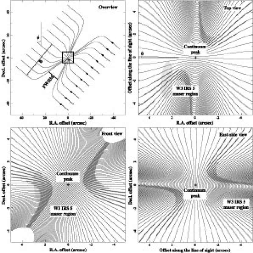
Figure 5: Hourglass model of the magnetic field in the W3 IRS 5 region. The angle $\theta\sim$ 2^∘ is the angle of inclination with respect to the sky plane, $\phi\sim$ 50^∘ the position angle, $A/B$ the pinch ratio ($A\>=$ 5″, $B\>=$ 35″) and $FWHM\>=$ 10″ the FWHM width of the the pinch at the location of the water masers. The all of the definitions are the same as those described in figure 7 of Robert et al.  (1993). A square (10″$\times$10″) in the overview panel indicates the area zoomed up and described in other three sub-panels. Thick parts of the magnetic field lines in the zoomed-up front view sub-panel indicate the locations where the field line have position angles 65^∘ $\leq\;PA_{\mbox{\tiny M}}\;\leq$ 85^∘. The location and the area of the W3 IRS 5 water maser region are indicated by a gray ellipse. The area center is located at 2″.5, $-$0″.5, and $-$2″.0 in R.A., decl., and line-of-sight offsets, respectively. The orientation of the ellipse major axis indicates the direction of the outflow found in the maser region (see figure 6 and 7 of Paper I). Thick parts of the magnetic field lines in the zoomed-up top and east-side views indicate the locations where the field line have inclinations 45^∘ $\leq\;|\theta_{\mbox{\tiny M}}|\;\leq$ 60^∘.

In this paper, we propose an hourglass model of the magnetic field shown in figure 5. This model is made to explain the magnetic field on the small scale ($<$ 10″), and consistent the large scale magnetic field ($\sim$ 1′) observed by RCTG and Greaves, Murray, & Holland (1994). The modeled field is pinched-in at the peak of the 800-µmcontinuum emission. Ladd et al. (1993) observed the 450-µm/800-µmcontinuum emission with a 7″-beam (a pointing accuracy of 2″), and found that the peak of the emission has a position offset of $\sim$ $-$2″.5 in R.A. and $\sim$ $+$0″.5 in decl. with respect to the center of the maser cluster. Although the continuum emission peak should coincide with the ¹³CO and C¹⁸O emission peaks (Oldham et al., 1994; Tieftrunk et al., 1995; Roberts, Crutcher, & Troland, 1997), the observed position is somewhat uncertain because of the large beams. It is possible that the C¹³O emission peak observed by Roberts, Crutcher, & Troland (1997) traces a segment of the outflow while the continuum emission peak traces the densest part of the parent molecular cloud. Tieftrunk et al. (1995) found four gas clumps traced by C³⁴S $J=$3–2 and $J=$5–4 emission, but none of the emission peaks coincides with the pinch center.

The magnetic field projection on the sky ($PA\>\sim$ 76^∘) mentioned in the previous sub-section is well consistent with that in the proposed magnetic field model (see figure 5b). Taking into account that the magnetic field vector is oriented toward the observer (a negative value of the measured Zeeman effect, STR; STCR), the maser region is likely located in front of the major axis of the hourglass (see figure 5c, d). The inclination of the magnetic field to the line of sight, however, cannot be completely consistent with the model, in which the inclination significantly varies from a point to another in the whole maser region.

The alignment of the magnetic field in the coverage of about 1″$\times$4″ in the water maser region provides a constraint on the pinch ratio of the hourglass model around $A/B\>\sim$ 0.14, as well as on the pinch width around $FWHM\>\sim$ 10″) (definitions of $A$ and $B$ are given in the caption of figure 5). As discussed by RCTG, one obtains a magnetic field strength of $\sim$1.3 mG at the pinch center when assuming a strength of the total undisturbed magnetic field of 25 $\mu$G and considering the $r^{-2}$ dependence of the magnetic field. This value is one order of magnitude smaller than that obtained by STR and STCR ($\sim$ 30 mG) but one order of magnitude larger than that estimated by RCTG. Crutcher (1999) found an empirical relation of a magnetic field strength, $B\>\propto\>n^{0.47}$, over a large range of gas densities $n$ up to 10⁷ cm^-3. Therefore, it is expected that the field strength found in the water maser cloud ($n\>\gtrsim$ 10⁸–10⁹ cm^-3) is consistent with the $B$–$n$ law (c.f. STR). STCR also pointed out that the magnetic field in the interstellar space (preshock region) should be enhanced in the maser region (postshock region) by a factor of $\sim$ 20.

4.3 The magnetodynamically super-critical collapse of the parent molecular cloud of W3 IRS 5

The origin of the magnetic field pinch is still obscured. The direction of the whole magnetic field is almost parallel to a molecular outflow found in W3 A (Mitchell, Maillard, & Hasegawa, 1991; Hasegawa et al., 1994). Momose et al. (2001) pointed out that a magnetic field would control the direction of a molecular outflow rather than that the magnetic field is influenced by the outflow. In W3 IRS 5, however, although the magnetic field seems to along the molecular outflow on a larger scale ($\sim$ 1′), it may not necessarily be parallel to the outflows on a smaller scale ($\sim$ 5″) as seen in the water masers. We evaluated the energy densities of the magnetic field and of the outflow of W3 IRS 5 using the same equations described in Momose et al. (2001). The critical magnetic field strength, $B_{\mbox{\tiny critical}}$, at which the field has the same energy density as that of the cylindrical outflow, is expressed by

$$B_{\mbox{\tiny critical}}\;=\left(\frac{8E_{\mbox{\tiny flow}}}{r^{2}l}\right)^{1/2},$$ (2)

where $E_{\mbox{\tiny flow}}$, $r$ and $l$ are the kinetic energy, the radius, and the total length of the cylindrical outflow, respectively. Adopting the total outflow energy estimated by Hasegawa et al. (1994), $E_{\mbox{\tiny flow}}\>\simeq$ 1.2$\times$10⁴⁶ erg, and the radius and the length of the outflow estimated by Mitchell, Maillard, & Hasegawa (1991), $r\>\simeq$ 4.1$\times$10¹⁷ cm and $l\>\simeq$ 2.5$\times$10¹⁸ cm, respectively (assuming the distance to W3 IRS 5 of 1.8 kpc here), we obtained $B_{\mbox{\tiny critical}}\>\simeq$ 0.48 mG, which is larger than the maximum strength observed in the HI Zeeman effect by RCTG ($\lesssim$ 0.22 mG). To obtain $B_{\mbox{\tiny critical}}$ for the water maser cloud, we converted equation (2) to,

$$B_{\mbox{\tiny critical}}\;=\;(8\pi\rho_{\mbox{\tiny maser}}v_{\mbox{\tiny maser}}^{2})^{1/2},$$ (3)

where $\rho_{\mbox{\tiny maser}}\>\gtrsim$  3.3$\times$10^-14 g cm^-3 (corresponding to $n_{\mbox{\tiny H${}_{2}$}}\>=$ 10⁸ cm^-3) is the gas density of the maser region necessary for maser excitation, $v_{\mbox{\tiny maser}}$ is the outflow velocity. Adopting the outflow velocity $v_{\mbox{\tiny maser}}\>\sim$ 15 km s^-1, we obtained $B_{\mbox{\tiny critical}}\>\simeq$ 250 mG. Thus, the magnetic field strength estimated on the basis of the Zeeman splitting ($\simeq$ 30 mG, STR) is one order of magnitude lower than the critical strength. This suggests that the magnetic cannot control the outflow dynamics.

This evaluation is consistent with that made for the W51M region by LLD. On the other hand, there is no observational evidence that the outflow controls the magnetic field structure. Momose et al. (2001) suggested that the magnetic field is aligned more in the younger phase of star-formation than in the more evolved one so that the disturbance of the former magnetic field due to the small-scale turbulence is not significant yet. This suggestion supports that W3 IRS 5 should be at the very early stage of star formation. Oldham et al. (1994) and Tieftrunk et al. (1995) estimated the mass of the molecular cloud associated with W3 IRS 5 to be 800–900 $M_{\sun}$. This value is still larger than the magnetodynamically-critical mass of 510 $M_{\sun}$ for a cloud with a radius of 9000 AU (corresponding to 5″ at 1.8 kpc) and a magnetic field strength of 30 mG. This indicates that the magnetic field of the W3 IRS 5 cannot support the gravity of the molecular cloud, in other words, that a part of the W3 IRS 5 cloud is collapsing under the magnetodynamically super-critical condition (Shu, Adams, & Lizano, 1987).

Note that the above evaluation is still consistent with the suggestion that the magnetic field should control the water maser excitation (Elitzur, Hollenbach, & McKee 1989, 1992; STCR). To consider the maser excitation, the velocity dispersion of the postshock region where the masers are excited, $\sigma_{v}\>\lesssim$ 0.6 km s^-1, is inserted instead of $v_{\mbox{\tiny maser}}$ in equation 3 (Paper I, II; STCR). Then one can estimate $B_{\mbox{\tiny maser}}\>\simeq$ 10 mG, smaller than or equal to the observed magnetic field strength.

It is still unclear what kind of object exists in the pinch center of the magnetic field. Tieftrunk et al. (1995) found four molecular gas clumps in W3 IRS 5, but none of the clumps is located at the pinch center. It is likely that these clumps were formed in the common parent molecular cloud and are responsible for the observed magnetic field. The magnetic field which controlled the multiple clumps supports the mild pinch ratio $A/B\>\simeq$ 0.14 rather than the extremely small ratio $A/B\>\simeq$ 0.04 speculated by RCTG.

5 Summary

Polarimetric VLBI observations of water masers in W3 IRS 5 have revealed that observed EVPAs of water masers features are well aligned in the whole maser region except for a small number of maser features. The directions of the magnetic field projected on the sky in the maser region are estimated to be perpendicular to the directions of the linear polarization of the masers ($PA\>\sim$ 76^∘). The magnetic field estimated supports the hourglass magnetic field model proposed previously. Thus, water maser linear polarization may reveal in detail the magnetic fields of the interstellar medium in star-forming regions. The W3 IRS 5 water maser region has a position offset from the pinch center of the hourglass and its magnetic field is unlikely to control the outflow dynamics. All of these observational facts suggest that the W3 IRS 5 cloud is collapsing under magnetically super-critical condition and that the outflows are not yet developed enough to completely disturb the magnetic field in this cloud. The hourglass structure of the magnetic field is suggested to be formed as a result of the collapse of the parent molecular cloud that is magnetically super-critical.

Table 1: Parameters of the water maser features toward W3 IRS 5.

Maser feature	Offset		LSR velocity (km s-1)		Peak Intensity	$P$	EVPA	Maser feature
(W3 IRS 5: I2003)	R.A. (mas)	decl. (mas)	Peak	Width	(Jy beam-1)	(%)	(deg)	(W3 IRS 5: I2000)
1	$-$1.50	3.33	$-$56.0	1.7	0.04	…	…	…
2	1075.72	1016.29	$-$43.1	3.8	18.41	11.0	$-$12.1	…
3	$-$389.93	$-$661.34	$-$42.9	1.7	7.78	…	…	…
4	0.08	$-$0.99	$-$42.6	1.3	6.95	…	…	…
5	$-$1.49	3.36	$-$42.1	3.8	111.05	0.8	$-$15.1	…
6	$-$388.32	$-$665.56	$-$42.0	2.1	9.60	0.7	19.8	…
7	$-$388.08	$-$671.67	$-$41.7	0.8	3.63	…	…	…
8	$-$431.85	$-$620.46	$-$41.7	0.8	1.48	…	…	29
9	$-$387.87	$-$667.89	$-$41.3	0.4	0.50	…	…	…
10	$-$0.01	$-$0.09	$-$41.3	1.3	26.10	…	…	…
11	$-$18.42	0.16	$-$40.7	1.7	8.95	…	…	…
12	$-$17.26	$-$1.79	$-$40.5	1.3	2.63	…	…	…
13	$-$1.37	4.38	$-$40.5	1.7	8.69	…	…	…
14	0.00	0.00	$-$40.5	5.1	79.89	0.8	$-$14.9	…
15	$-$1.66	5.47	$-$40.3	1.3	8.91	…	…	…
16	$-$0.37	$-$11.64	$-$40.0	2.5	20.81	…	…	…
17	$-$3.92	5.23	$-$39.6	0.4	5.05	…	…	…
18	$-$387.50	$-$670.38	$-$39.3	4.2	9.99	0.8	$-$17.8	…
19	$-$386.67	$-$677.37	$-$38.9	3.0	7.25	…	…	…
20	$-$4.28	8.23	$-$38.8	1.3	5.63	…	…	…
21	$-$3.78	7.50	$-$38.8	0.8	3.91	…	…	…
22	$-$6.27	8.67	$-$38.2	3.8	26.49	0.7	$-$11.8	…
23	9.72	$-$16.39	$-$37.8	2.1	11.11	12.8	$-$11.4	…
24	$-$386.73	$-$676.74	$-$37.7	1.3	0.29	…	…	…
25	$-$7.97	13.24	$-$37.5	1.7	1.88	…	…	…
26	$-$9.20	14.11	$-$36.9	1.7	2.14	…	…	…
27	786.55	1792.69	$-$36.7	2.1	10.01	1.1	$-$15.5	64
28	797.51	1750.03	$-$36.2	0.8	0.56	…	…	65
29	783.13	1802.02	$-$35.8	3.8	14.81	0.9	$-$18.0	66
30	787.03	1794.17	$-$35.5	5.1	91.10	0.4	$-$12.5	63
31	328.54	$-$2001.74	$-$35.0	1.7	2.24	…	…	71
32	796.47	1750.38	$-$35.0	3.0	0.53	…	…	…
33	$-$416.12	$-$600.11	$-$34.6	4.2	11.55	…	…	…
34	$-$1.46	3.30	$-$34.6	0.4	0.11	…	…	…
35	$-$0.02	$-$0.02	$-$34.6	0.4	0.06	…	…	…
36	$-$6.21	8.51	$-$34.6	0.4	0.08	…	…	…
37	794.01	1751.23	$-$34.5	0.4	2.10	…	…	…
38	794.65	1750.92	$-$34.1	0.4	0.23	…	…	79
39	295.92	$-$2025.00	$-$33.9	1.7	0.94	…	…	73
40	294.72	$-$2025.82	$-$33.8	2.5	4.43	5.4	$-$5.0	76
41	293.69	$-$2027.11	$-$33.7	0.8	1.06	…	…	…
42	331.95	$-$2004.59	$-$33.7	1.3	6.95	7.0	89.6	…
43	325.76	$-$1999.60	$-$33.6	4.6	21.89	7.3	30.4	82
44	332.52	$-$2004.95	$-$33.3	0.8	4.25	12.9	$-$79.2	…
45	$-$415.21	$-$602.42	$-$33.2	3.0	1.00	…	…	…
46	334.25	$-$2006.04	$-$33.1	3.0	10.90	8.4	$-$59.1	83
47	$-$415.45	$-$604.25	$-$33.0	3.4	3.84	…	…	…
48	324.56	$-$1998.90	$-$32.9	5.9	13.12	…	…	…
49	324.99	$-$1998.91	$-$32.4	2.1	6.56	1.5	$-$62.5	…
50	795.87	1750.48	$-$32.3	2.1	1.93	…	…	…
51	326.65	$-$1999.60	$-$32.0	1.3	0.19	…	…	77
52	331.83	$-$2004.52	$-$31.2	0.4	0.05	…	…	…
53	249.87	$-$2079.93	$-$30.4	4.6	4.02	…	…	91
54	228.02	$-$2083.62	$-$29.9	1.7	1.05	…	…	94
55	230.35	$-$2083.38	$-$29.9	0.8	0.44	…	…	98
56	229.26	$-$2083.48	$-$29.9	0.4	0.01	…	…	…
57	227.05	$-$2083.52	$-$29.9	1.7	1.09	…	…	…
58	325.72	$-$1999.57	$-$29.6	2.1	0.06	…	…	…
59	795.39	1750.80	$-$29.5	1.3	0.13	…	…	…
60	$-$503.83	$-$2377.04	$-$23.8	3.0	0.58	…	…	…
61	$-$205.57	$-$1830.29	$-$6.8	2.1	1.32	…	…	…

Water maser features detected toward W3 IRS 5. The feature is designated as W3 IRS 5:I2003 N, where N is the ordinal source number given in this column (I2003 stands for sources found by Imai et al.  and listed in 2003).
Relative value with respect to the location of the position-reference maser feature: W3 IRS 5:I2003 14.
A channel velocity spacing multiplied by a number of detected maser spots in the feature.
Fraction of linear polarization intensity to total intensity.
The feature identical to that found in Paper I, W3 IRS 5:I2000 M, where M is the ordinal source number given in this column.

References

- Abraham & Vilas Boas (1994) Abraham, Z., & Vilas Boas, J. W. S. 1994, A&A, 290, 956
- Akujor et al. (1993) Akujor, C. E., Spencer, R. E., Zhang, F. J., Fanti, C., Ludke, E., & Garrington, S. T. 1993, A&A, 274, 752
- Barvainis & Deguchi (1989) Barvainis, R., & Deguchi, S. 1989, AJ, 97, 1089
- Crutcher (1999) Crutcher, R. M. 1999, ApJ, 520, 706
- Claussen et al. (1994) Claussen, M. J., Gaume, R. A., Johnston, K. J., & Wilson, T. L. 1994, ApJ, 424, L41
- Deguchi & Watson (1990) Deguchi, S., & Watson, W. D. 1990, ApJ, 354, 649
- Deguchi & Watson (1986a) –. 1986a, ApJ, 302, 750
- Deguchi & Watson (1986b) –. 1986b, ApJ, 302, 108
- Diamond (1995) Diamond, P. J. 1995, in ASP Conf. Ser. 82, VERY LONG BASELINE INTERFEROMETRY AND THE VLBA, ed. J. A. Zensus, P. J. Diamond, & P. J. Napier (San Francisco: ASP), 227
- Elitzur (1992) Elitzur, M. 1992a, in Astronomical Masers (Dordrecht: Kluwer)
- Elitzur (1992) –. 1992b, ARA&A, 30, 75
- Elitzur, Hollenbach, & McKee (1989) Elitzur, M., Hollenbach, D. J., & McKee, C. F. 1989, ApJ, 346, 983
- Elitzur, Hollenbach, & McKee (1992) –. 1992, ApJ, 394, 221
- Evans II (1999) Evans II, N. J. 1999, ARA&A, 37, 311
- Feigelson & Montmerle (1999) Feigelson, E. D., & Montmerle, T. 1999, ARA&A, 37, 363
- Goldreich, Keeley, & Kwan (1973) Goldreich, P., Keeley, D. A., & Kwan, J. Y. 1973, ApJ, 179, 111
- Greaves, Murray, & Holland (1994) Greaves, J. S., Murray, A. G., & Holland, W. S. 1994, A&A, 284, L19
- Genzel & Downes (1977) Genzel, R., & Downes, D. 1977, A&AS, 30, 145
- Gwinn (1994) Gwinn, C. R. 1994a, ApJ, 429, 241
- Gwinn (1994) –. 1994b, ApJ, 429, 253
- Gwinn, Moran, & Reid (1992) Gwinn, C. R., Moran, J. M., & Reid, M. J. 1992, ApJ, 393, 149
- Hasegawa et al. (1994) Hasegawa, T. I., Mitchell, G. F., Mattews, H. E., & Tacconi, L. 1994, ApJ, 426, 215
- Hayashi, Kobayashi, & Hasegawa (1989) Hayashi, M., Kobayashi, H., & Hasegawa, .T. 1989, ApJ, 340 298
- Heiles et al. (1993) Heiles, C., Goodman, A. A., McKee, C. F., & Zweibel, E.G. 1993, in Protostar and Planets III, ed. E. H. Levy, & J. I. Lunine (Tucson: Univ. Arizona Press.), 279
- Hollenbach, Elitzur, & McKee (1993) Hollenbach, D. J., Elitzur, M., & McKee, C. F. 1993, in Astrophysical Masers, ed. A. W. Clegg, & G. E. Nedoluha (Heidelberg: Springer), 159
- Hollenbach & McKee (1989) Hollenbach, D., & McKee, C. F. 1989, ApJ, 342, 306
- Horiuchi, Migenes, & Deguchi (2000) Horiuchi, S., Migenes, V., & Deguchi, S. 2000, in Astrophysical Phenomena Revealed by Space VLBI, Proceedings of the VSOP Symposium, eds. H. Hirabayashi, P. G. Edwards, & D. W. Murphy, (Sagamihara, Japan: ISAS), 105
- Horiuchi & Kameya (2000) Horiuchi, S., & Kameya, O. 2000, PASJ, 52, 545
- Imai, Deguchi, & Sasao (2002) Imai, H., Deguchi, S., & Sasao, T. 2002, ApJ, 567, 971 (Paper II)
- Imai et al. (2000) Imai, H., Kameya, O., Sasao, T., Miyoshi, M., Deguchi, S., Horiuchi, S., & Asaki, Y. 2000, ApJ, 538, 751 (Paper I)
- Ladd et al. (1993) Ladd, E. F., Deane, J. R., Sanders, D. B., & Wynn-Williams, C. G. 1993, ApJ, 419, 186
- Leppänen, Liljeström, & Diamond (1998) Leppänen, K., Liljeström, T., & Diamond, P.J. 1998, ApJ, 507, 909 (LLD)
- Marscher et al. (2002) Marscher, A. P., Jorstad, S. G., Mattox, J. R., & Wehrle, A. 2002, ApJ, 577, 85
- McKee et al. (1993) McKee, C. F., Zweobe, E. G., Godman, A. A., & Heiles, C. 1993, in Protostar and Planets III, ed. E. H. Levy, & J. I. Lunine (Tucson: Univ. Arizona Press.), 327
- Mitchell, Maillard, & Hasegawa (1991) Mitchell, G. F., Maillard, J.-P., & Hasegawa, T. I. 1991, ApJ, 371, 342
- Momose et al. (2001) Momose, M., Tamura, M., Kameya, O., Greaves, J. S., Chrysotomou, A., Hough, J. H., & Morino, J.-I. 2001, ApJ, 555, 855
- Oldham et al. (1994) Oldham, P. G., Griffin, M. J., Richardson, K. J., & Sandell, G. 1994, A&A, 284, 559
- Reid (1995) Reid, M. J. 1995, in ASP Conf. Ser. Vol. 82, Very Long Baseline Interferometry and the VLBA, ed. J. A. Zensus, P. J. Diamond, & P. J. Napier (San Francisco: ASP), 209
- Reid & Moran (1981) Reid, M. J., & Moran, J. M. 1981, ARA&A, 19, 231
- Roberts, Crutcher, & Troland (1997) Roberts, D. A., Crutcher, R. M., & Troland, T. H. 1997, ApJ, 479, 318
- Roberts et al. (1993) Roberts, D. A., Crutcher, R. M., Troland, T. H., & Goss, W. M. 1993, ApJ, 412, 675 (RCTG)
- Sarma et al. (2002) Sarma, A. P., Troland, T. H., & Crutcher, R. M., & Roberts, D. A. 2002, ApJ, 580, 928 (STCR)
- Sarma, Troland, & Romney (2001) Sarma, A. P., Troland, T. H., & Romney, J. D. 2001, ApJ, 554, L217 (STR)
- Shu, Adams, & Lizano (1987) Shu, F. H., Adams, F. C., & Lizano, S. 1987, ARA&A, 25, 23
- Tieftrunk et al. (1997) Tieftrunk, A. R., Gaume, R. A., Claussen, M. J., Wilson, T. L., & Johnston, K. J. 1997, A&A, 318, 931
- Tieftrunk et al. (1995) Tieftrunk, A. R., Wilson, T. L., Steppe, H, Gaume, R. A., Johnston, K. J., & Claussen, M. J. 1995, A&A, 303, 901
- Torrelles et al. (2001) Torrelles, J. M., Patel, N. A., Gómez, J. F., Ho, P. T. P., Rodoríguez, L. F., Anglada, G., Garay, G., Greenhill, L. J., et al. 2001a, Nature, 411, 277
- Torrelles et al. (2001) –. 2001b, ApJ, 560, 853
- Troland et al. (1989) Troland, T. H., Crutcher, R. M., Goss, W. M., & Heiles, C. 1989, ApJ, 347, L89