Unusual CO Line Ratios and kinematics in the N83/N84 Region of the Small Magellanic Cloud

Abstract

We present new CO ($1\rightarrow 0$) and ($2\rightarrow 1$) observations of the N83/N84 molecular cloud complex in the south–east Wing of the Small Magellanic Cloud (SMC). While the ($2\rightarrow 1$)/($1\rightarrow 0$) integrated line brightness ratio (in temperature units) is uniformly 0.9 throughout most of the complex, we find two distinct regions with unusually high ratios ($2\rightarrow 1$)/($1\rightarrow 0$)$\gtrsim 2$. These regions are associated with the N84D nebula and with the inside of the 50 pc expanding molecular shell N83. This shell is spatially coincident with the NGC 456 stellar association and the HFPK2000–448 radio continuum/X–ray source tentatively classified as a supernova remnant. We explore possible causes for the high ratios observed and conclude that the CO emission probably arises from an ensemble of small ($R\sim 0.1$ pc), warm ($T_{g}\sim 40$ K) clumps. Analysis of the CO shell parameters suggests that it is wind–driven and has an age of slightly more than 2 million years. We have also used this dataset to determine the CO–to–H₂ conversion factor in the SMC, an especially interesting measurement because of the low metallicity of this source ($\approx 1/9$ solar). Surprisingly, after comparing the CO luminosities of clouds in N83/N84 with their virial masses, we find a CO–to–H₂ conversion factor X_CO only $1.9$ times larger than what we obtain when applying the same algorithm to solar metallicity clouds in the Milky Way and M 33. This result fits into the emerging pattern that CO observations with high linear resolution suggest nearly Galactic values of X_CO in a wide range of environments.

1 Introduction

The Magellanic Clouds —with their unobscured lines of sight, their small internal extinction, and their profusion of star-forming sites— constitute excellent laboratories for the study of the interaction between massive stars and their environment. They are also the nearest metal–poor systems with active star–formation ( $Z_{LMC}\sim Z_{\odot}/4$ and $Z_{SMC}\sim Z_{\odot}/9$ for the Large and the Small Cloud respectively; Dufour, 1984; Kurt & Dufour, 1998). As such, they provide invaluable insight into the physics and chemistry of the interstellar medium (ISM) in primitive galaxies.

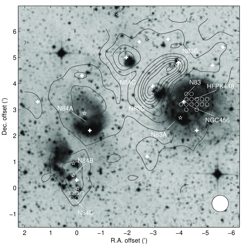
Figure 2: CO ($2\rightarrow 1$) integrated intensity map overlaid on the annotated DSS optical image of the N83/N84 region. The different symbols indicate: IR sources in the SIMBAD database (stars), molecular clouds listed in Table 1 (crosses), and individual pointings with high ¹²CO ($2\rightarrow 1$)/($1\rightarrow 0$) ratio (circles). The labels indicate the approximate positions of the emission line nebulosities listed in the Henize (1956) catalog, as well as two sources associated with the expanding molecular shell: the NGC 456 stellar association and the HFPK2000-448 radio continuum peak/SNR. The white circle in the bottom right corner indicates the resolution of the CO map, identical to that of Figure 1.

In this work we will discuss some of the molecular gas properties and kinematics in the N83/N84 region of the Small Magellanic Cloud (Henize, 1956, Figure 2). This region is especially interesting because it is one of the few isolated, yet relatively active star-forming regions in the otherwise inconspicuous SMC Wing. It comprises several CO clouds (Mizuno et al., 2001; Israel et al., 2003), H II regions (Henize, 1956; Davies et al., 1976), various early–type stars (Testor & Lortet, 1987), and an expanding shell coincident with both the NGC 456 stellar association and a possible supernova remnant (source 448 in Haberl et al., 2000, henceforth HFPK2000-448 (catalog )). This expanding shell appears to be interacting with the nearby molecular cloud, sweeping and compressing an important mass of molecular hydrogen (at least $10^{4}$ M_⊙; c.f., §3.3.2), and perhaps setting up a second generation of star formation. If N 83 indeed contains a supernova remnant, it represent one of a handful of opportunities to study the interaction between a molecular cloud and a SNR in a metal poor environment.

Recently, Bolatto et al. (2000) have reported the detection of unusually high ¹²CO ($2\rightarrow 1$)/ ($1\rightarrow 0$)$\sim 3$ ratios in the molecular envelope of the N159/N160 complex in the Large Magellanic Cloud (LMC). Such high ratios are rarely observed in the Galaxy and are interesting because they convey information on the structure of the ISM in these systems (c.f., §3.1). Bolatto et al. suggested that these high ratios are a direct consequence of the low metallicity of the medium. If this is the case, we expect them to be more pronounced in regions with strong UV radiation fields and even lower metallicity. We undertook the present study in order to search for anomalous ¹²CO ($2\rightarrow 1$)/($1\rightarrow 0$) ratios in a region of very low metallicity, and thus to verify how widespread such ratios are. A second motivation was to attempt to further distinguish between the mechanisms that can cause such ratios.

The present study also allows us to revisit the problem of estimating molecular masses using CO observations in metal–poor systems. Low heavy–element abundances cause lower dust–to–gas ratios in a low metallicity ISM ($D/G\sim Z^{1-2}$; Lisenfeld & Ferrara, 1998). Because dust particles are efficient absorbers of UV light, they shield molecules from dissociative radiation. Thus, the lower dust–to–gas ratios in the SMC ($D/G_{SMC}\sim 1/30\,D/G_{MW}$; Stanimirovic et al., 2000, and references therein) lead us to expect higher rates of molecular photodissociation. This is particularly true for molecules such as CO, where lower metallicities also imply lower column densities, hence significantly smaller self-shielding. Indeed, it has long been known that emission from molecules is much fainter in dwarf galaxies, which tend to be low metallicity systems (e.g., Taylor, Kobulnicky, & Skillman, 1998).

Because of these effects, exactly how CO emission traces the molecular ISM in metal-poor systems remains uncertain, and it has stayed a goal of extragalactic CO observations to characterize this relationship. Since the early days of CO observations in the Galaxy astronomers have derived CO–H₂ calibrations and used them to compute H₂ column densities and masses (e.g., Sanders, Solomon, & Scoville, 1984; Bloemen et al., 1986; Dame, Hartmann, & Thaddeus, 2001, and references therein). The factor to convert ¹²CO integrated intensities into H₂ column densities is referred to as $\mbox{\rm X${}_{\rm CO}$}={\rm N(\mbox{\rm H${}_{2}$})/I(\mbox{\rm${}^{12}$CO})}$, and has been determined using the virial theorem, X–ray shadowing experiments, and an array of other techniques. As it is notoriously difficult to incorporate all of the relevant physics (such as cloud structure and optical depth) into model calculations, astronomers have relied on empirical calibrations of X_CO rather than on a–priori determinations.

Since its introduction, it has been clear that X_CO must be a function of the local conditions of the ISM or at least the average properties of the cloud ensemble; some of the most relevant quantities are thought to be radiation field, dust–to–gas ratio, and metallicity. There are several calibrations of X_CO with metallicity available in the literature (Dettmar & Heithausen, 1989; Wilson, 1995; Arimoto, Sofue, & Tsujimoto, 1996; Israel, 1997, 2000; Bolatto, Jackson, & Ingalls, 1999; Barone et al., 2000; Boselli, Lequeux, & Gavazzi, 2002). These all agree that decreases in ISM metallicity and dust–to–gas ratio should result in noticeable increases in X_CO, meaning a lower CO integrated intensity per unit H₂ column density. They differ, however, in their estimates just how large these increases in X_CO will be. In particular, observational studies find that X_CO appears to depend strongly on the attained linear resolution. Studies based on observations with high linear resolution, such as that provided by interferometers, tend to find smaller increases in X_CO in metal–poor galaxies than those accomplished with larger beams (e.g. Wilson, 1995; Walter et al., 2001, 2002; Rosolowsky et al., 2003). Based on comparisons with far infrared dust emission, Israel (2000) has ascribed these effects to intrinsic observational bias.

2 Observations

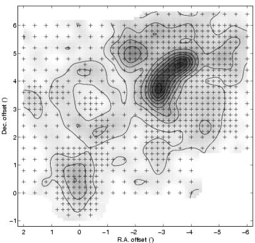
Figure 1: Integrated intensity CO ($2\rightarrow 1$) map, showing the sampling. The contour levels start at 1 and go in steps of 1 to 8 K km s^-1. This map was produced using gaussian interpolation, smoothing to a final beam size of 38″ HPBW. The offsets are with respect to $\alpha_{1950}=1^{\rm h}13^{\rm m}23\fs 1,\delta_{1950}=-73^{\circ}36\arcmin 33\arcsec$ ($\alpha_{2000}=1^{\rm h}14^{\rm m}45\fs 3,\delta_{2000}=-73^{\circ}20\arcmin 42\arcsec$).

Carbon monoxide emission from the N83/N84 region was first detected and subsequently mapped by Israel et al. (1993, 2003) as part of the ESO-SEST Key Programme “CO in the Magellanic Clouds.” Because of considerable improvements in millimeter receiver sensitivity in the years since, it has become possible to use SEST to make large maps of relatively faint sources in a reasonable period of time. It has also become possible to simultaneously observe the ($1\rightarrow 0$) and ($2\rightarrow 1$) transitions of CO, allowing us to obtain reliable line ratios. We mapped a region of $\sim 10\arcmin\times 9\arcmin$ encompassing N83, N84, and HFPK2000-448, simultaneously at 115.271204 and 230.542408 GHz (Figure 1). We detected over a dozen clouds in this area. The properties of the peak ($2\rightarrow 1$) spectra from these clouds are compiled in (Table 1).

We acquired the maps in November 2000, by using SEST 115/230 GHz dual SIS receiver and feeding the two frequencies into the split high–resolution acousto–optical spectrometer (AOS) backend. The resulting bandpasses ($\sim 50$ km s^-1 for 230 GHz and $\sim 100$ km s^-1 for 115 GHz) easily accomodated the narrow lines and small velocity variations inside the molecular complex. The spectra were obtained using double–beam–switching mode, with a chop of 11.5′ in azimuth. The few spectra contaminated by emission in the off position were reobserved at a different hour angle. According to its documentation, SEST has HPBW(230)$\approx 23\arcsec$ and HPBW(115)$\approx 45\arcsec$, and its main beam efficiencies are $\eta_{mb}(230)\approx 0.50$ and $\eta_{mb}(115)\approx 0.70$. We initially mapped a 24″ grid (i.e., approximately full–beam spacing at 230 GHz) and refined this to a 12″ grid in regions of bright emission and those regions in which we wished to increase the signal–to–noise ratio. We used a nearby SiO maser to determine pointing and focus corrections before each observing session. The SEST pointing accuracy is 3″ RMS. Assuming a 63 kpc distance to the SMC, the scale of these observations is $\approx 18$ pc per arcminute.

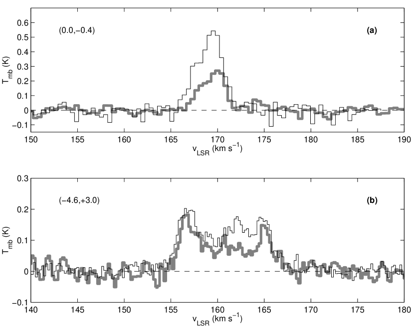
Figure 4: (a) CO ($1\rightarrow 0$) (thick line) and ($2\rightarrow 1$) (thin line) toward the region south of N84 (N84D), corrected by their respective main beam efficiencies and with the higher transition convolved to the angular resolution of the lower one. Remarkably similar velocity structure, and a line ratio $\sim 2.0$. (b) Same toward the CO expanding shell, with both transitions convolved to 1′ resolution. The ($2\rightarrow 1$) transition is enhanced in the center component, corresponding to gas filling the inside of the shell.

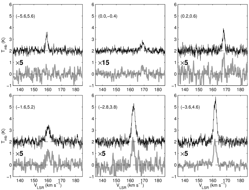
Figure 5: ¹²CO and ¹³CO ($2\rightarrow 1$) spectra obtained near several peaks in the integrated intensity map. The pointing near the N84D region with offsets $(+0.0,-0.4)$, where we observe ¹²CO ($2\rightarrow 1$)/($1\rightarrow 0$) ratio $\sim 2.0$, was also observed. This position was chosen because of its relatively strong ¹²CO emission. Unfortunately, repeating the ¹³CO observations toward other pointings with high ratios would have required very long integrations.

To compare the ($2\rightarrow 1$) and ($1\rightarrow 0$) data, we convolved the spectra of both transitions to a common angular resolution, thus removing the effect of the different beam size of the observations. We found unusually high ¹²CO($2\rightarrow 1$)/($1\rightarrow 0$) line ratios in two regions of the map (Figure 2). The first instance occurs just south of N84, close to the IRAS 01133–7336/N84D H II region (Figure 4a). The second region is found in the gas inside the expanding shell N 83, which is associated with NGC 456 and HFPK2000-448 (Figure 4b). To determine the optical depth $\tau_{21}$ of the ($2\rightarrow 1$) emission we obtained ¹³CO ($2\rightarrow 1$) spectra toward several positions (Figure 5). Table 2 summarizes our observations, as well as our results for $\tau_{21}$ obtained assuming N(¹²CO)/N(¹³CO)$\sim 40-90$ (c.f., §3.1.3).

3 Discussion

3.1 The Origin of the Unusually High Line Ratios

Optically thick CO emission arising from thermalized gas at $T>10$ K yields a brightness-temperature ratio ($2\rightarrow 1$)/($1\rightarrow 0$)$\sim 1$. Deviations from these conditions —for example, lower temperatures or subthermal excitation in gas with volume densities below the critical density of the ($2\rightarrow 1$) transition, $n_{crit}\sim 10^{4}$ cm^-3— generally produce ratios less than unity. However, somewhat higher ratios, ($\sim 1.2$) are frequently found in LMC and SMC molecular clouds (Israel et al., 2003, and references therein). These are probably caused by a mixture of high and low optical depths in molecular clouds and cloud envelopes (i.e., a departure from the assumption of a homogeneous source characterized by a single temperature and a single column density).

Unusually high ¹²CO ($2\rightarrow 1$)/($1\rightarrow 0$) ratios were observed by Bolatto et al. (2000) in the LMC, who discussed four possible origins for them: 1) self–absorbed ¹²CO ($1\rightarrow 0$)emission, 2) optically thin emission from isothermal gas, 3) ensembles of small, optically thick isothermal clumps, and 4) optically thick emission with temperature gradients. With the available data they were not able to unequivocally determine the cause of the high ratio, although self–absorbed CO emission appeared unlikely. The same causes may explain the high ratios we find in the N83/N84 region of the SMC. In this Section, we describe each of these mechanisms and explore how well they can account for the new data on the SMC.

3.1.1 Self–absorbed emission

Self–absorption is caused by an intervening envelope of colder CO in the line of sight, which produces a dip in the background CO spectra. This effect is more prominent for lower $J$ transitions, since most of the intervening cold gas will be found near the ground state. The spectra obtained toward the region south of N84 clearly show that the ¹²CO ($1\rightarrow 0$) transition is not suppressed by self–absorption. Fig.  4 demonstrates that the two transitions have the same line profile, thus convincingly showing they arise from the same parcels of gas.

3.1.2 Optically thin emission

It can be shown that for gas in local thermodynamic equilibrium (LTE) the ratio of optical depths in the ($1\rightarrow 0$) and ($2\rightarrow 1$) transitions is

$$\frac{\tau_{21}}{\tau_{10}}=2\frac{\left({1-e^{-\frac{2h\nu_{10}}{kT_{ex}}}}\right)}{\left({e^{\frac{h\nu_{10}}{kT_{ex}}}-1}\right)},$$ (1)

where $\tau_{10}$ and $\tau_{21}$ are the opacities of the respective transitions, $\nu_{10}$ is the frequency of the lower transition, $T_{ex}$ is the excitation temperature, and $k$ and $h$ are Boltzmann’s and Planck’s constants. Since the opacity of rotational transitions is proportional to the square of their rotation quantum number $J$ at high temperatures, optically thin warm gas can produce ($2\rightarrow 1$)/($1\rightarrow 0$) ratios $\leq 4$. The emission from such regions will be faint, and observations in the Galactic plane may be biased against finding them, which may explain why it is easier to find them in the Magellanic Clouds. However, we clearly detected emission from ¹³CO in the same place south of N 84 where we measured a high ¹²CO ($2\rightarrow 1$)/($1\rightarrow 0$)$=2.0\pm 0.2$ ratio (Figure 5). Although the observed ¹²CO/¹³CO ($2\rightarrow 1$)$\approx 20$ ratio is somewhat high, it nevertheless indicates that this transition is optically thick unless the carbon isotopic abundance ratio is much lower in the SMC than in the Galaxy. The best available determinations of isotopic abundance ratios in the SMC suggest that N(¹³C)/N(¹²C)$\sim 40-90$, although data are scarce (Heikkilä, Johansson, & Olofsson, 1999). In Table 2 we summarize our optical depth results for several clouds in the complex. The range of $\tau_{21}$ values listed in the last column are calculated assuming the quoted limits from Heikkilä, Johansson, & Olofsson (1999).

For the pointing at ($+0.0,-0.4$) we find an opacity in the range $\tau_{21}\sim 1.5-4.4$, indicating that the ($2\rightarrow 1$) emission there is optically thick. If the N(¹²CO)/N(¹³CO) column density ratio turns out to be significantly lower than 40, however, the emission could be optically thin. Such a scenario could conceivably result from the combined effects of chemical fractionation and selective photodissociation in the ISM. Heikkilä, Johansson, & Olofsson (1999), for example, determined this ratio to be $\sim 15$ in the N27 region of the SMC using a mean escape probability radiative transfer code modeling spherical clouds.

3.1.3 Emission from very small warm clumps

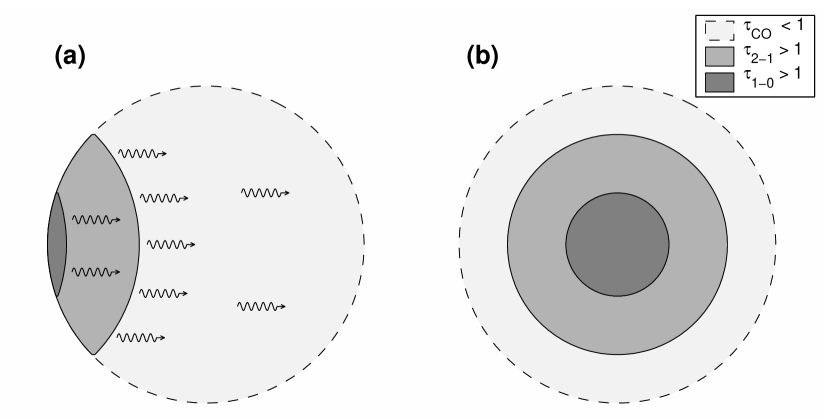
Figure 6: A small, constant density, constant excitation spherical clump model, showing the geometry of the $\tau=1$ surfaces for the CO ($2\rightarrow 1$) and ($1\rightarrow 0$) transitions for an observer located (a) to the far right of the clumplet, and (b) in front of the clumplet. The very lightly shaded area surrounded by the dashed line is optically thin in both transitions and contributes a small (albeit not negligible) amount to the brightness of the clump in either transition. The darker shaded areas indicate the regions where first the ($2\rightarrow 1$) and then the ($1\rightarrow 0$) transitions accrue enough column density to become optically thick. Most CO photons arise from these surfaces. Small, warm clumps fill more of the beam in the higher, more opaque CO transitions.

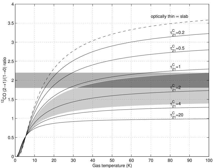
Figure 7: CO ($2\rightarrow 1$)/($1\rightarrow 0$) ratio for clumps of different central ($2\rightarrow 1$) opacity $\tau^{C}_{21}$, similar those of Figure 6, plotted against gas kinetic temperature. Note tha the overall opacity of an spherial, constant density clump is 33% higher than $\tau^{C}$, which is the clump radius in opacity units. The calculations use LTE, assuming that the volume density is high enough to thermalize the lower CO transitions ($n\gtrsim 10^{4}$ cm^-3), and include the effect of the optically thin portion of the clump. The shaded areas represent the observational constraints for the region south of N83 where high ratios were found, as discussed in the main text (¹²CO ($2\rightarrow 1$)/($1\rightarrow 0$)$\approx 2$, $\tau_{21}\sim 1.5-4.4$).

Collections of very small, isothermal, optically thick clumplets also have the potential to produce high ¹²CO ($2\rightarrow 1$)/($1\rightarrow 0$) ratios. They do so partially through a beam filling effect; because of the faster growth of the ($2\rightarrow 1$) opacity with column density the optically thick region of the clumps appears larger in the higher transitions, thus filling more of the beam. Figure 6 illustrates the geometry of this effect, in which the optically thick $\tau_{21}=1$ “photosphere” of the clump is larger and occurs closer to its surface than the $\tau_{10}=1$ “photosphere.” Perhaps more importantly, small clumps provide a natural geometry that allows the ($2\rightarrow 1$) transition to become optically thicker than the ($1\rightarrow 0$) transition. The line ratios for a spherical geometry can be easily computed under the assumption of local thermodynamic equilibrium (LTE); this is probably a safe assumption if the clumps have volume densities in excess of $n\gtrsim 10^{4}$ cm^-3 (because of the critical density $n_{crit}\propto J^{3}$, it is extremely difficult to obtain a high ($2\rightarrow 1$)/($1\rightarrow 0$) ratio with subthermal excitation unless the equivalent radiation temperature is higher than the gas temperature, which is not usually the case in mm–wave radio astronomy). For each transition, we assumed a constant gas temperature and density and numerically integrated to find the opacity, $\tau(r)$, in a clump as a function of $r$, the projected distance to the center. The results of these calculations as a function of the gas temperature, $T_{g}$, and the central clump opacity, $\tau^{C}$, are shown in Figure 7. The shaded regions represent the observational constraints: the measured ¹²CO ($2\rightarrow 1$)/($1\rightarrow 0$) ratio and the central clump opacity derived from the ¹²CO/¹³CO ($2\rightarrow 1$) measurements as described in the previous paragraph. The observations constrain the gas temperature to be strictly $T_{g}>30$ K and more likely $T_{g}\gtrsim 40$ K. The clump radius is constrained to be $\tau^{C}\sim 1$ in opacity units for the ($2\rightarrow 1$) transition. This opacity translates into a physical column density $N(\mbox{\rm${}^{12}$CO})\sim 1.5\times 10^{17}$ cm^-2 at $T_{g}\sim 40$ K, which can be converted to a length of $R\sim 0.1$ pc by assuming that all the carbon is locked in the CO molecules with a carbon abundance of $\log({\rm C/H})\approx-4.7$ (Garnett et al., 1995; Kurt & Dufour, 1998) and that the volume density is $n_{H_{2}}\approx 10^{4}$ cm^-3 (i.e., about the critical density of the ($2\rightarrow 1$) transition). The resulting parameters thus indicate fairly standard, but very warm, clumps. The heating is presumably provided by the star cluster found near the high-ratio region (source 166 of Bica & Schmitt, 1995) or by the adjacent H II region and IR source (IRAS 01133–7336; Figure 2).

The appeal of the “small warm clumps” scenario is twofold: 1) it naturally explains why it is easier to find high line ratios in systems of low metallicity, such as the LMC and SMC, and 2) as it has predictive power, it can easily be falsified. Indeed, we have shown that clump radii have to be small in opacity units to produce large ratios. If the physical sizes of clumps do not change with metallicity, low CO column densities will be more common in lower metallicity systems because of the lower abundances of carbon and oxygen. If the abundance of CO scales by a factor similar to that of the metallicity, then a clump with central opacity $\tau^{C}(\mbox{\rm${}^{12}$CO})\sim 4$ in the Milky Way would have $\tau^{C}(\mbox{\rm${}^{12}$CO})\sim 0.5$ in the SMC. The “small warm clumps” model requires that the ¹³CO ($2\rightarrow 1$)/($1\rightarrow 0$) ratio be $\sim 3-4$ in this source, and it can be used to predict the intensities of the higher CO transitions. The model also requires that the N(¹²CO)/N(¹³CO) column density ratio be $\sim 40-50$ south of N84.

3.1.4 Optically thick regions with large temperature gradients

High brightness ratios can, in principle, also be produced by optically thick gas if the $\tau=1$ surfaces of each transition occur in regions of different temperature. To reproduce the observations, we need a ratio of excitation temperatures $T_{ex}(\tau_{21})/T_{ex}(\tau_{10})\gtrsim 2$. How large a temperature gradient does this change represent? Using the LTE approximation we computed the column densities of CO necessary to attain $\tau=1$ for each transition at different temperatures. We used this information to obtain a very rough estimate of the typical increment in column density $\Delta N(\mbox{\rm${}^{12}$CO})$ required to go from the $\tau_{21}=1$ surface at $T$, to the $\tau_{10}=1$ surface at $T/2$. We found that a reasonable estimate is $\Delta N(\mbox{\rm${}^{12}$CO})\sim 10^{16}$ cm^-2. Taking into account the abundance of carbon, this is equivalent to a change in visual extinction $\Delta\mbox{\rm A${}_{\rm V}$}\sim 0.05$. Since CO becomes the main reservoir of carbon at $\mbox{\rm A${}_{\rm V}$}\gtrsim 1$, this means that the cloud turns optically thick in the ($1\rightarrow 0$) transition at a depth only $\sim 5\%$ larger than that at which the $\tau_{21}=1$ surface is found. To explain the observations, however, we require the excitation temperature of the gas to drop by a factor of two for this $\sim 5\%$ change in depth. Gas temperature profiles computed for PDRs externally heated by UV sources show that such gradient is extremely unlikely (e.g., Hollenbach & Tielens, 1999). This simple argument is also supported by line ratios obtained from self–consistent PDR calculations. At no point in the parameter space of a homogeneous, externally heated PDR is the CO $\mbox{($2\rightarrow 1$)}/\mbox{($1\rightarrow 0$)}>1.8$, and ratios greater than unity only occur at very high densities and radiation fields (Kaufman, Wolfire, Hollenbach, & Luhman, 1999). Perhaps embedded IR sources with no UV flux, such as protostars, could produce the heating necessary to obtain the right temperature ratio without the associated photodissociation of CO. This appears very unlikely, however, since these sources would have to occur at a particular depth, coincident with the $\tau_{21}=1$ surface.

We have explored four possible explanations for the unusually high ¹²CO ($2\rightarrow 1$)/($1\rightarrow 0$) ratios observed south of the N84 region. We have shown that two mechanisms, self–absorption and optically thin emission, are improbable. Of the remaining two, small warm clumps and optically thick gas with large temperature gradients, we prefer the first, although it is not possible to entirely discard the second with the present data. High line ratios could also conceivably originate in the optically thin portion of clumps with density gradients (for example, critical Bonnor–Ebert spheres). The proper modeling of such objects, however, requires a full self–consistent radiative transfer and temperature profile calculation, and is beyond the scope of this paper: nevertheless we note that warm temperatures will still be necessary to produce high line ratios. In addition, the relevant ratios are also obtained if we allow completely inhomogeneous models. One of the simplest examples would be a population of cold, dense clumps surrounded by a warm, tenuous envelope. Unfortunately, a model containing only two completely independent components already has a minimum of eight free parameters, which greatly exceeds the number of constraining observational parameters (three in our case). We may decrease the number of free parameters somewhat by making plausible assumptions, but even in that case would we need more constraints than we presently have. Future observations may remedy this.

3.2 The Expanding Molecular Shell

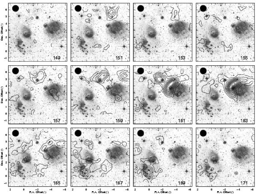
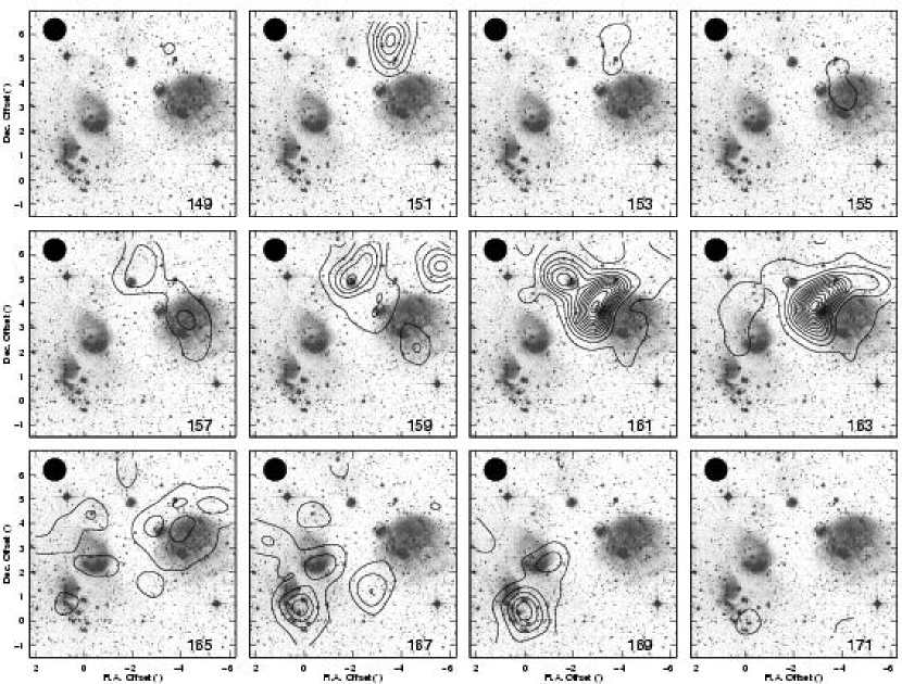
Figure 3: Channel maps of the CO emission for the ($1\rightarrow 0$) (top group of twelve panels) and ($2\rightarrow 1$)(bottom) transition, convolved to the same angular resolution (55″) and overlaid on the DSS image of the region. The contours are identical for both transitions: starting at 0.2 and increasing by 0.2 K km s^-1. The ratio of main beam temperatures is uniformly $\approx 1$ throughout the map, except in the two regions indentified in Figure 2.

The second instance of unusually high ¹²CO ($2\rightarrow 1$)/($1\rightarrow 0$) ratios in the N83/N84 region occurs in a remarkable place: the inside of the expanding shell–like structure associated with NGC 456 and HFPK2000-448 (Figure 2). This optical shell has a molecular counterpart apparent in a careful inspection of Figure 3. Starting at velocities 155–157 km s^-1 the center of N83 lights up, while at 161 km s^-1 the eastern rim emits brightly in CO. At 165 km s^-1, some emission shows up at the center of the shell in the maps of the ($2\rightarrow 1$) transition. The spectrum obtained over the central 1′ of this structure even more clearly exhibits this kinematic signature (Figure 4b). While the emission associated with the walls of the shell has very similar brightness temperature in the ($1\rightarrow 0$) and ($2\rightarrow 1$) transitions, the gas inside the shell appears brighter in the ($2\rightarrow 1$) transition by a factor of $\sim 2$. The shell is $\sim 50$ pc in diameter, and the molecular material associated with it is expanding at a velocity $\sim\pm 6.5$ km s^-1. The northern and eastern edges of the shell are sharp and well defined in the optical pictures, while its southwestern edge appears ragged and soft. The cause of this difference in appearance is strikingly clear in the CO channel maps: along the northern and eastern edges, the expansion of the shell is contained by a molecular cloud at $\mbox{V${}_{\rm LSR}$}\sim 163$ km s^-1, while the south and west sides appear able to expand more freely. It is not immediately clear whether this bright CO cloud (corresponding to peaks MP 5 and MP 7 in Table 1) consists of swept-up matter, or represents an ambient cloud interacting with the expanding shell.

A question arises: is the expanding shell due to a supernova explosion, or is it a wind–driven structure? The classification by Haberl et al. (2000) of HFPK2000-448 as a SNR was tentative, and based on the detection of coincident radio continuum emission at 13 cm and X–Ray emission by ROSAT. Extended X–ray emission and/or extended nonthermal radio continuum are telltale evidence for SNRs. However, in the case of HFPK2000-448 the data are not conclusive. The X–ray emission could be extended but the quality of this determination (as measured by its likelihood parameter) is low, and there is no detection of the radio continuum at other frequencies to confirm that the spectral index is nonthermal.

In any case, the rather modest expansion measured in CO is hard to reconcile with the much higher expansion speeds expected from a supernova remnant. It is quite in line, however, with the much lower speeds that should characterize wind–driven shells. From the interstellar bubble model by Weaver et al. (1977), we find that the age, $t$, of the bubble is related to its radius, $R_{s}$, in parsecs and its expansion velocity, $V_{s}$, in km s^-1 by $t=6\times 10^{5}R_{s}/V_{s}$. With a radius of about 25 pc and an expansion velocity of 6.5 km s^-1, the age of the bubble should be about 2.3 million years. From the model we also find the relation between mechanical wind-luminosity, $L_{w}$, in erg s^-1 and original ambient total hydrogen density, $n_{H}$, in cm^-3 to be $L_{w}/n_{H}=7.65\times 10^{46}R^{5}/t^{3}$. By conservatively assuming $L_{w}/L_{bol}=10^{-3}$ for the ratio between mechanical wind and stellar bolometric luminosities, we may reduce this to $L_{bol}/n_{H}=6\times 10^{37}\,{\rm ergs}^{-1}{\rm cm}^{3}=1.5\times 10^{4}{\rm L}_{\odot}{\rm cm}^{3}$. If the total stellar luminosity of the embedded association NGC 456 is of the order of $10^{7}$ L_⊙, the original ambient density should have been of the order $n_{H}\approx 650$ cm^-3. These luminosities and original densities seem quite reasonable for a luminous association dispersing its molecular birthcloud. It is also not unreasonable to suppose that a massive member of the association turned supernova within a few million years. If such an event indeed occurred, the resulting remnant should rapidly have filled the wind–blown bubble that we have observed. Consequently, the chemistry and excitation around N 83 could be dominated by SNR–caused shocks, even though the overall kinematics of the shell would still be those of a wind–driven structure. We found no evidence, however, of uncommon mm–line ratios in the N83B/C molecular cloud. Its ¹²CO ($2\rightarrow 1$)/($1\rightarrow 0$) ratio is $\sim 0.9$, identical to that of the rest of the complex, and our observations of HCO⁺ ($1\rightarrow 0$) toward offsets ($-3.6,4.6$) yield a ratio ¹²CO/HCO⁺ $\approx 18\pm 2$, similar to that reported by Heikkilä, Johansson, & Olofsson (1999) toward the SMC source N27.

It would be of considerable interest to confirm the SNR identification of N 83/HFPK2000-448. If it is confirmed, N 83 in the SMC would be very similar to the well-established SNR N 49 in the LMC, which also appears to be interacting directly with a molecular cloud (Banas et al., 1997). N 83 would represent another excellent opportunity to study molecular cloud–SNR interactions in a metal-poor environment, complementing studies of similar interactions within the Galaxy. Indeed, notwithstanding the fact that most Type II supernovae must occur within their parent clouds and despite their potential importance as triggers of a secondary wave of star–formation activity (Opik, 1953), there are only a handful of such molecular cloud–SNR associations identified in the literature (e.g., Cornett, Chin, & Knapp, 1977; Wootten, 1977; Wilner, Reynolds, & Moffett, 1998; Kim et al., 1998; Dubner et al., 1999, and references therein). Most of these interactions lie in the Galactic plane, where obscuration and confusion pose observational difficulties that are largely absent in the Magellanic cluds.

3.3 The X_CO Factor in N83/N84

3.3.1 Measuring Cloud Properties

To measure the individual cloud properties we proceeded as follows: from the individual map spectra we constructed uniformly sampled main beam intensity data cubes in the CO ($2\rightarrow 1$) and ($1\rightarrow 0$) transitions using the COMB built–in 2D gaussian interpolation. The cubes have angular resolutions (HPBW) of $35\arcsec$ and $55\arcsec$, respectively, corresponding to spatial resolutions of $11$ pc and $17$ pc. Their velocity resolution is 0.25 km s^-1. After convolving the ($2\rightarrow 1$) cube to the resolution of the ($1\rightarrow 0$) cube, we carried out a pixel–by–pixel comparison of the two cubes and found that the best linear relation between both datasets was $\mbox{\rm I${}_{\rm CO}$}\mbox{($1\rightarrow 0$)}=0.9\,\mbox{\rm I${}_{\rm CO}$}\mbox{($2\rightarrow 1$)}$, very similar to other results obtained for Magellanic Cloud objects (c.f. Israel et al., 2003, and references therein). This scaling will be used later to compute molecular masses using CO ($2\rightarrow 1$) observations.

We proceeded to identify clouds in the channel maps, and then measured three properties for each cloud: its size, its velocity dispersion, and its integrated CO intensity. From the first two quantities we calculated a virial mass for each cloud, which we compared to the mass derived from the integrated intensity using the Galactic CO–to–H₂ conversion factor. To obtain these numbers we specified a threshold intensity, then built a mask that started from a seed position and velocity, and included neighboring regions of the data cube with two adjacent velocity channels above this threshold. We defined a “cloud” as an unmasked region contiguous in $\alpha-\delta-v$ space. This is a practical definition that is similar or identical to those employed in a number of other studies (e.g. Solomon et al., 1987; Heyer et al., 2001; Rosolowsky et al., 2003). The threshold intensity was varied over a wide range, and cloud properties were computed for each of its values. Obviously, very high values of the threshold will select only small regions within a cloud, while low values will tend to merge clouds together, and even lower values will include positive noise as emission. We determined the reasonable range of values to use for each cloud by observing when the cloud properties experienced a “jump” caused by the mask growing into a neighboring cloud.

After identifying an individual cloud, we calculate its size, velocity dispersion, and CO flux as follows. To obtain the size, we compute the second moment of the integrated brightness distribution of the cloud in the $\alpha-\delta$ plane (i.e., the RMS size). Because the moment underestimates the true size for gaussian clouds, we include a correction factor that depends on the ratio of the threshold intensity used to the peak intensity of the cloud. The inclusion of this factor is important for two reasons: 1) in cases of confusion and low signal–to–noise, it allows us to estimate the properties of an entire cloud from the portion that is easily identifiable, and 2) it avoids oversubtraction in our beam deconvolution. It assumes, however, that the cloud is gaussian in position–velocity space. Fortunately, this assumption can be veryfied by observing how the cloud properties change as a function of threshold intensity (they should be constant), and it appears to hold for the clouds here studied. From the corrected second–moment values, we “deconvolve” the beam by subtracting its size from the measured cloud size in quadrature. Finally, we apply the factor of $\frac{3.4}{\sqrt{\pi}}$ (Solomon et al., 1987) to convert from the RMS size to the radius of a theoretical spherical cloud (this factor can be readily motivated by considering a constant density spherical cloud and comparing the RMS size to the spherical radius). Along with an assumed SMC distance of 63 kpc (see Walker 1998; Cioni et al. 2000), this treatment results in a physical cloud size given by the formula:

$$R_{sph}\approx 0.41\sqrt{\sigma_{\alpha}^{2}+\sigma_{\delta}^{2}-2\sigma_{beam}^{2}},$$ (2)

where $\sigma_{\alpha}$ and $\sigma_{\delta}$ are the threshold–corrected RMS sizes of the cloud in the $\alpha$ and $\delta$ directions, $\sigma_{beam}$ is the RMS size of the beam (all measured in arcseconds), and $R_{sph}$ is the spherical radius of the cloud in parsecs.

Other works, in particular those focused on Milky Way clouds, have treated clouds as ellipsoids and used the corresponding form of the virial theorem due to Bertoldi & McKee (1992). This approach is problematic in extragalactic astronomy, because the observations do not have many resolution elements across the cloud and their signal–to–noise is low. Under these conditions deconvolution becomes very difficult and the precise shape of the source is hard, if not impossible, to recover. Therefore, we content ourselves with measuring a single size parameter and considering the simple model of a spherical cloud.

We calculate both the threshold–corrected RMS velocity dispersion, $\sigma_{v}$, and the equivalent width, $EW$, from the integrated spectrum of each cloud. For the equivalent width, we employ the definition of Heyer et al. (2001),

$$EW=\frac{\Sigma_{i}\psi(v_{i})}{\mbox{Max}(\psi(v_{i}))}$$ (3)

where $\psi(v_{i})$ is the spectrum of the cloud in question. For a gaussian distribution, $EW=1.06\,FWHM$. Because it does not diverge when signal–free noise is added to the edge of a spectrum, this linewidth measure is more robust than the second moment as a measure of the RMS velocity dispersion. Moreover, by comparing these two measures we get a good idea of how well a spectrum is approximated by a gaussian (for our data, the ratio $EW/\sigma_{v}$ correlates very well with the $\chi^{2}$ value of a gaussian fit to a spectrum).

We compute the CO luminosity by summing the intensities of the entire cloud and again applying a correction factor based on the peak–to–threshold ratio and an assumed gaussian profile. In the case of the CO ($2\rightarrow 1$) data cube, we applied the aforementioned $0.9$ conversion factor to calculate the corresponding CO ($1\rightarrow 0$) luminosity for the cloud: essentially, we used the ($2\rightarrow 1$) measurements as predictors of the ($1\rightarrow 0$) intensities, taking advantage of their higher S/N and spatial resolution. To compute molecular cloud masses (including the contribution by He) we use the formula

$${\rm M_{mol}}=\mbox{$\alpha_{\rm CO}$}\,S_{\rm CO}\,d^{2},$$ (4)

where $S_{\rm CO}=\int\mbox{\rm I${}_{\rm CO}$}\,d\Omega$ is the spatially integrated ¹²CO flux of the molecular cloud measured in Jy km s^-1, $\mbox{$\alpha_{\rm CO}$}=1.07\times 10^{4}$ $M_{\odot}$ Mpc^-2 (Jy km s^-1)^-1 (corresponding to a canonical conversion factor $\mbox{\rm X${}_{\rm CO}$}=2\times 10^{20}$ cm^-2 (K km s^-1)^-1 ), and $d$ is the distance to the SMC in Mpc.

We compute the virial masses using the assumption that each cloud is spherical and virialized with a density profile of the form $\rho\propto r^{-1}$. Thus the virial mass is given by the formula (Solomon et al., 1987)

$${\rm M_{vir}}=1040\,\sigma_{v}^{2}\,R_{sph},$$ (5)

where $\sigma_{v}$ is the RMS cloud velocity dispersion in km s^-1, $R_{sph}$ is the spherical cloud radius in pc, and M_vir is the cloud’s virial mass in M_⊙.

3.3.2 Results

We have applied the procedure described above to several subsets of the data, as well as the whole datacube. We focused our attention on three clouds contained in the Nyquist–sampled regions of our original dataset, roughly corresponding to MP7, MP10, and MP13 in Table 1 (i.e., the clouds associated with N83B/C, N84C, and N84B/D respectively; Fig. 2). We also computed masses for what we call the “northern region” (the complex encompassing N83B/C and N84C but not including MP6, which appears to be an unrelated cloud peaking a much lower velocities), and for the complex as a whole. Our results are summarized in Table 3. Because the dominant sources of uncertainty in our determination of cloud masses are the cloud boundary definitions, we repeated the procedure described above for a wide variety of thresholds. Thus, we probed the properties of the complex on a variety of size scales, and on each scale we estimated a reasonable range of values for each of the physical parameters. In Table 3 we give the properties of structures on scales ranging from what seem to be compact, self–gravitating object to complexes composed of a few large, bound, virialized clouds connected by low surface brightness filaments.

How do the results obtained from the ($2\rightarrow 1$) data compare with those from the more commonly observed ($1\rightarrow 0$) transition? CO ($1\rightarrow 0$) usually provides the basis for estimating X_CO in the SMC and other galaxies, even though the lower spatial resolution at $115$ GHz makes size measurements more difficult. We performed identical analyses on both datasets. For the most part, the $115$ GHz properties were similar to those derived from the $230$ GHz data, though the CO flux and linewidth of MP10 are both notably larger at $115$ GHz. The complex, as a whole, has somewhat higher linewidth (and consequently virial mass) when measured in the ($1\rightarrow 0$) transition. This is artificial and caused by the higher noise of the ($1\rightarrow 0$) datacube: to encompass the same area used in the ($2\rightarrow 1$) calculations we need to use too low a threshold, causing positive noise to be included as emission.

Because of the higher resolution and better signal–to–noise, we prefer the results from the ($2\rightarrow 1$) data. Assuming all clouds share the same conversion factor, these results yield $\mbox{\rm X${}_{\rm CO}$}\approx 7.0\pm 3.4\times 10^{20}$ cm^-2 (K km s^-1)^-1 (i.e., $3.5\pm 1.7$ times the Galactic value) on the size scale of individual molecular clouds ($\sim 10$ pc). Using this conversion factor, the total molecular mass traced by CO in the complex is $M(\mbox{\rm H${}_{2}$})\sim 2.5\times 10^{5}$ M_⊙.

We believe our algorithm to be both robust and simple. It is designed to be easily applicable to a heterogeneous set of observations. However, because several details (particularly the masking correction) differ from those previous works, our results (particularly our size measurements) may not be readily comparable to those in the literature. To account for this, we applied our algorithm to both the Rosette Molecular Cloud (Williams, Blitz, & Stark, 1995) and a subset of well resolved solar metallicity clouds from the BIMA survey of M 33 (Rosolowsky et al., 2003). Both of these tests yielded values for X_CO of $3.4-4.0\times 10^{20}$ cm^-2 (K km s^-1)^-1. In light of this, our result can be restated as follows: our measurments of the X_CO factor in the SMC yield a value for X_CO $1.9\pm 0.9$ times the value of X_CO obtained for identical measurements on the Rosette Molecular Cloud and several M 33 clouds.

How do these molecular masses and estimates of X_CO compare to those obtained by other studies of the SMC? The results presented here are consistent with those obtained independently by Israel et al. (2003), taking into consideration that they mapped only part of the complex in the ($1\rightarrow 0$) CO transition, with generally lower signal–to–noise ratios. Our ($2\rightarrow 1$) result is lower by about a factor of $\sim 2$ than the average value X_CO$\sim 12\times 10^{20}$ cm^-2 (K km s^-1)^-1 obtained by Rubio et al. (1993) from SEST CO ($1\rightarrow 0$) measurements of clouds elsewhere, in the southwest Bar of the SMC. However, when we adjust the sizes of Rubio et al. (1993) to match our own definition and include beam deconvolution, we find a $\sim 40\%$ reduction in the average size of a cloud. The corresponding drop in cloud virial masses suggests a value of X_CO$\sim$ 6—8$\times 10^{20}$ cm^-2 (K km s^-1)^-1  consistent with our estimates. We also take the opposite approach, bringing our results into line with their measurements by considering the properties of the N83 complex at the $0.4$ K km s^-1integrated intensity contour. If we reject the low velocity emission, as Rubio et al. (1993) did for several clouds, and employ their definitions and formulae then we obtain a conversion factor of X_CO$\sim 20\times 10^{20}$ cm^-2 (K km s^-1)^-1, in excellent agreement with their average result for complexes ($23\times 10^{20}$ cm^-2 (K km s^-1)^-1). This value is also in agreement with that obtained by Mizuno et al. (2001) using the NANTEN telescope, with a beam size HPBW$\approx 2\farcm 6$.

3.3.3 Caveats and Limitations

We note that most common limitations inherent to the data such as low signal–to–noise, blended line profiles, and low spatial resolution will drive our estimate of X_CO toward higher rather than lower numbers. All the usual caveats regarding the applicability of the virial theorem apply, with the added concern that we are considering a particularly active region. The effects of an expanding shell and active star formation on nearby clouds, although not immediately apparent from the data, may be important.

We should caution that virial estimates of X_CO on the large scales are suspect. First, they require assuming that the entire complex is virialized and that large scale motions (e.g., galactic rotation, expanding shells) are negligible. Second, the mass on the spatial scale of the measurement has to be dominated by molecular hydrogen, meaning that the contributions from stars and H I are negligible. The ATCA+Parkes HI observations of this region (Stanimirovic et al., 1999), for example, show that the atomic hydrogen mass in a 120 pc diameter region centered on the N83/N84 complex is $\sim 530\times 10^{3}$ M_⊙, very similar to our virial mass estimate. Because this is an integral along the line–of–sight, however, it is impossible to assert how much of this mass is really associated with the complex. Third, they require assuming that the velocity field inside the region is uniformly traced by CO emission, otherwise the intensity–weighted second moment usually employed to obtain the velocity dispersion is meaningless.

Finally, we have gauged the magnitude of the conversion factor indepently from virial considerations by following the method outlined by Israel (1997). We use his SMC calibration $N_{\rm H}/\sigma(FIR)=1.65\times 10^{28}{\rm cm}^{-2}({\rm Wm}^{-2}{\rm sr}^{-1})^{-1}$ to derive the molecular mass from the far infrared emission near the N83/N84 complex. At 15′ resolution, the temperature–corrected far–infrared surface brightness is $\sigma(FIR)=7\times 10^{-7}{\rm Wm}^{-2}{\rm sr}^{-1}$ (Schwering, 1988; Schwering & Israel, 1990) so that $N_{\rm H}=1.2\times 10^{22}{\rm cm}^{-2}$. Both the old H I map by McGee & Newton (1981) and the newer ATCA+Parkes data by Stanimirovic et al. (1999) yield a mean neutral hydrogen column density of $N_{\rm HI}=5.5\times 10^{21}{\rm cm}^{-2}$. From this we deduce the molecular hydrogen column density $N_{\rm H2}=3.2\times 10^{21}{\rm cm}^{-2}$, corresponding to a molecular gas fraction $2N_{\rm H2}/(N_{\rm H}+N_{\rm He})=0.4$, which is not unusual for a star–forming region. The CO luminosity integrated over the N 83/N 84 complex is given by Mizuno et al. (2001) as $L_{\rm CO}=1.3\times 10^{4}\mbox{K~{}km~{}s${}^{-1}$}{\rm pc}^{2}$. As this luminosity is beam-independent for unresolved sources, we can easily extrapolate to the 15′ resolution of the molecular hydrogen column density just derived. At that resolution, the CO integral corresponding to the observed CO luminosity would be $I_{\rm CO}=0.22\mbox{K~{}km~{}s${}^{-1}$}$. This is probably an underestimate, because such a large beam would encompass additional H II regions most likely associated with their own CO clouds. Our best estimate – to be verified by future CO mapping of the area – is therefore $I_{\rm CO}=0.33\pm 0.11\mbox{K~{}km~{}s${}^{-1}$}$, yielding an independent estimate $\mbox{\rm X${}_{\rm CO}$}=100\pm 50\times 10^{20}$ cm^-2 (K km s^-1)^-1  very similar to the other X_CO values of the SMC found in the same way (Israel, 1997).

These results fit well into an apparently consistent pattern. Observations with high linear resolutions, i.e. single–dish observations of nearby extragalactic objects such as those presented here or interferometric observations of more distant objects, consistently suggest virial cloud masses implying nearly Galactic X_CO conversion factors regardless of environment. By contrast, observations not resolving individual clouds but covering whole complexes have suggested much higher conversion factors in metal–poor systems. This pattern may be explained in several ways: 1) it may be caused by a large “mm–dark” molecular mass in metal–poor galaxies, comprised by H₂ clouds without CO emission. In this scenario the observed CO emission arises only from the densest, most shielded clouds in a complex. If this is true, CO observations suffer from a severe observational bias. 2) It is possible that the complexes observed are not virialized, or their masses dominated by unaccounted–for stellar or atomic gas components, and that there is not a great deal of hidden molecular mass. In this case, high–resolution observation such as those presented here, suggest that individual clouds are virialized with an approximately Galactic X_CO, indicating that metal–poor galaxies have molecule–poor ISMs.

If the complexes are virialized and their masses are dominated by the molecular gas, then their global dynamics would be better probes of the overall molecular mass than the dynamics of individual clouds. On the other hand, if complexes are not virialized or their masses not dominated by molecular gas, then there may be no way for CO observations to get a handle on the total molecular masses of metal–poor galaxies. In this case other tracers, such as far–infrared emission from dust, large surveys of UV H₂ line absorption, or FIR [C II] measurements, may be the only way of obtaining global molecular mass estimates. By themselves, CO observations are insufficient to distinguish between these two scenarios. Observations of other tracers, such as the far–infrared, will be necessary to establish whether CO is a good tracer in metal–poor galaxies.

4 Summary and Conclusions

We have presented new CO ($1\rightarrow 0$) and ($2\rightarrow 1$) observations of the N83/N84 nebulae in the SMC that show an active and complex region, home to several interesting astrophysical phenomena. We have identified 14 molecular clouds and an expanding molecular shell with a center coincident with the NGC 456 stellar association and the HFPK2000–448 radio continuum/X–ray source classified by Haberl et al. (2000) as a SNR. The shell is most likely wind–driven, and appears to have an age of 2.3 million years. We have also identified two extended regions of unusually high ($2\rightarrow 1$)/($1\rightarrow 0$) ratio: the first found south of the complex near the N84D emission line region, the second located inside the expanding molecular shell. A ¹³CO spectrum toward this first region shows that the ($2\rightarrow 1$) transition has opacity $\tau\approx 1.5-4.4$ assuming N(¹²CO)/N(¹³CO)$\sim 40-90$.

Barring the unlikely cases that the isotopic N(¹²C)/N(¹³C) carbon ratio is considerably lower than in the Galaxy or that fractionation effects have decreased the isotopomer N(¹²CO)/N(¹³CO) ratio to much below the isotopic ratio, this high line ratio is not caused by low optical depths. Inspection of the line profiles in Figure 4 also shows that the high ratio is not due to self–absorbed ($1\rightarrow 0$) emission. We have considered optically thick emission with temperature gradients, but some simple calculations show that the gradients required to reproduce the observed ratio are unrealistically large compared to those expected in photodissociation regions. Finally, we modeled the emission produced by an ensemble of spherical, isothermal clumps, and found that we can reproduce the observations with fairly warm ($T_{g}\sim 40$ K) but otherwise normal molecular clumps ($n\sim 10^{4}$ cm^-3, $R\sim 0.1$ pc). The high temperature required may explain why these high ratios are not more commonly observed.

We have also used the CO data to revisit the problem of the CO–H₂ conversion factor in the SMC. Using a simple and robust algorithm we found the X_CO factor in three clouds of the complex to be $\mbox{\rm X${}_{\rm CO}$}\approx 7.0\pm 3.4\times 10^{20}$ cm^-2 (K km s^-1)^-1 ($\mbox{\rm X${}_{\rm CO}$}\approx 3.5\pm 1.7$ times the Galactic value), estimated from the CO ($2\rightarrow 1$) data using virial calculations and supported by the results obtained from the ($1\rightarrow 0$) data. This value is about $1.9$ times that which we obtain when applying our algorithm to the Rosette Molecular Cloud and GMCs in M 33. The result is an X_CO that is considerably smaller than would be expected a priori for the very metal–poor SMC, which has a metallicity $Z\sim 1/9Z_{\odot}$. Higher values have been obtained from a CO/virial analysis of the complex as a whole, and higher yet from a non-virial, far-infrared analysis of the complex. These results are consistent with the pattern emerging from extragalactic observations over the last decade.

Table 1: CO ($2\rightarrow 1$) Molecular Peaks in the N83/N84 Region

Source	$\Delta\alpha$	$\Delta\delta$	Tpeak		Vlsr		FWHM		$\int T_{mb}\,dv$
	(′)	(′)	(K)		(km s-1)		(km s-1)		(K km s-1)
MP1	-5.6	+5.4	1.08$\pm$	0.06	159.29$\pm$	0.05	1.96$\pm$	0.12	2.2$\pm$	0.12
MP2	-5.2	+4.7	0.64$\pm$	0.02	163.84$\pm$	0.09	5.09$\pm$	0.22	3.44$\pm$	0.12
MP3	-4.6	+2.2	0.76$\pm$	0.04	158.46$\pm$	0.08	2.78$\pm$	0.19	2.18$\pm$	0.12
MP4	-4.1	+3.3	0.46$\pm$	0.02	156.31$\pm$	0.04	2.38$\pm$	0.09	1.14$\pm$	0.04
MP5	-3.9	+4.8	1.84$\pm$	0.04	162.26$\pm$	0.04	3.34$\pm$	0.09	6.4$\pm$	0.14
MP6	-3.5	+5.7	1.2$\pm$	0.02	151.27$\pm$	0.03	2.25$\pm$	0.06	2.82$\pm$	0.06
MP7	-2.9	+3.9	2.74$\pm$	0.02	162.32$\pm$	0.01	2.97$\pm$	0.03	8.6$\pm$	0.06
MP8	-2.7	+1.2	0.5$\pm$	0.02	166.53$\pm$	0.05	2.07$\pm$	0.13	1.08$\pm$	0.06
MP9	-2.4	+5.6	0.22$\pm$	0.04	159.48$\pm$	0.45	5.61$\pm$	1.05	1.22$\pm$	0.2
MP10	-1.9	+5.0	1.26$\pm$	0.04	160.16$\pm$	0.05	3.84$\pm$	0.11	5.28$\pm$	0.12
MP11	-0.5	+2.2	0.48$\pm$	0.02	167.81$\pm$	0.11	4.38$\pm$	0.27	2.2$\pm$	0.12
MP12	-0.2	+4.3	0.34$\pm$	0.02	164.19$\pm$	0.21	6.25$\pm$	0.5	2.02$\pm$	0.14
MP13	+0.0	+0.3	1.42$\pm$	0.04	168.01$\pm$	0.03	2.71$\pm$	0.07	4.06$\pm$	0.08
MP14	+1.5	+3.3	0.52$\pm$	0.04	167.12$\pm$	0.09	3.12$\pm$	0.22	1.68$\pm$	0.1

Table 2: Optical Depth Data

$\Delta\alpha$	$\Delta\delta$	Transition	Tpeak		Vlsr		FWHM		$\int T_{mb}\,dv$		$\tau$
(′)	(′)		(K)		(km s-1)		(km s-1)		(K km s-1)
-5.6	+5.6	12CO (2–1)	1.34$\pm$	0.04	159.26$\pm$	0.03	1.8$\pm$	0.07	2.52$\pm$	0.08
		13CO (2–1)	0.22$\pm$	0.08	$\cdots$		$\cdots$		0.1$\pm$	0.04	$1.0-3.5$
+0.0	-0.4	12CO (2–1)	0.78$\pm$	0.04	169.04$\pm$	0.06	2.57$\pm$	0.15	2.08$\pm$	0.1
		13CO (2–1)	0.04$\pm$	0.004	169.02$\pm$	0.15	2.48$\pm$	0.35	0.1$\pm$	0.012	$1.5-4.4$
+0.2	+0.6	12CO (2–1)	1.66$\pm$	0.06	167.98$\pm$	0.03	1.74$\pm$	0.07	2.96$\pm$	0.02
		13CO (2–1)	0.32$\pm$	0.04	167.91$\pm$	0.1	1.3$\pm$	0.23	0.42$\pm$	0.06	$6.1-13.8$
-1.6	+5.2	12CO (2–1)	1.14$\pm$	0.04	160.32$\pm$	0.07	3.89$\pm$	0.16	4.76$\pm$	0.16
		13CO (2–1)	0.16$\pm$	0.02	160.63$\pm$	0.17	4.58$\pm$	0.41	0.82$\pm$	0.06	$7.6-17.0$
-2.8	+3.8	12CO (2–1)	3.04$\pm$	0.02	162.45$\pm$	0.02	3.07$\pm$	0.03	9.84$\pm$	0.14
		13CO (2–1)	0.4$\pm$	0.02	162.05$\pm$	0.05	2.37$\pm$	0.11	0.96$\pm$	0.06	$4.0-9.2$
-3.6	+4.6	12CO (2–1)	3.5$\pm$	0.02	161.87$\pm$	0.01	2.57$\pm$	0.01	9.34$\pm$	0.12
		13CO (2–1)	0.4$\pm$	0.02	161.81$\pm$	0.03	2.36$\pm$	0.08	0.98$\pm$	0.02	$4.4-10.0$

Table 3: Cloud Properties

Quantity	MP 7	MP 10	MP 13	N. Region	Complex
CO ($2\rightarrow 1$)
$\alpha_{\mbox{off}}$	$-3\farcm 09$	$-1\farcm 75$	$+0\farcm 02$	$-3\farcm 00$	$-2\farcm 34$
$\delta_{\mbox{off}}$	$+3\farcm 98$	$+5\farcm 01$	$+0\farcm 39$	$+4\farcm 35$	$+3\farcm 62$
Velocity Centroid (km s-1)	$162.0$	$160.3$	$168.3$	$161.6$	$162.0$
Velocity Dispersion $\sigma_{v}$ (km s-1)	1.25	1.45	1.1	1.94	4.7/3.0
$R_{sph}$ (pc)	22	14	13.5	32	65
$S_{\rm CO}$ (Jy km s-1)	497	136	115	742	1,700
Mmol from CO ($10^{3}$ M⊙)	21	5.8	4.9	32	73
Mvir Virial Mass ($10^{3}$ M⊙)	35	29	18	126	1,500
${\rm M_{vir}}/{\rm M_{mol}}$	1.7	5.0	3.7	4.0	20
$\frac{\mbox{$\alpha_{\rm CO}$}}{\mbox{$\alpha_{\rm CO}$}(MW)}$	0.9	2.7	1.9	2.2	11
CO ($1\rightarrow 0$)
$\alpha_{\mbox{off}}$	$-3\farcm 10$	$-1\farcm 73$	$+0\farcm 24$	$-2\farcm 92$	$-1\farcm 91$
$\delta_{\mbox{off}}$	$+4\farcm 02$	$+5\farcm 03$	$+0\farcm 54$	$+4\farcm 43$	$+3\farcm 64$
Velocity Centroid (km s-1)	$162.2$	$160.0$	$168.4$	$161.5$	$162.2$
Velocity Dispersion $\sigma_{v}$ (km s-1)	1.2	2.0	1.25	2.2/1.8	4.2/3.2
$R_{sph}$ (pc)	21	15	16	35	72
$S_{\rm CO}$ (Jy km s-1)	440	193	132	715	1,500
Mmol from CO ($10^{3}$ M⊙)	19	8.2	5.6	30	63
Mvir Virial Mass ($10^{3}$ M⊙)	32	60	25	176	1,300
${\rm M_{vir}}/{\rm M_{mol}}$	1.7	7.3	4.5	5.8	21
$\frac{\mbox{$\alpha_{\rm CO}$}}{\mbox{$\alpha_{\rm CO}$}(MW)}$	0.9	3.9	2.4	3.1	11

References

- Arimoto, Sofue, & Tsujimoto (1996) Arimoto, N., Sofue, Y., & Tsujimoto, T. 1996, PASJ, 48, 275
- Banas et al. (1997) Banas K.R., Hughes J.P., Bronfman L., & Nyman L.-A., 1997, ApJ480, 607
- Barone et al. (2000) Barone, L. T., Heithausen, A., Hüttemeister, S., Fritz, T., & Klein, U. 2000, MNRAS, 317, 649
- Bertoldi & McKee (1992) Bertoldi, F. & McKee, C. F. 1992, ApJ, 395, 140
- Bica & Schmitt (1995) Bica, E. L. D. & Schmitt, H. R. 1995, ApJS, 101, 41
- Bloemen et al. (1986) Bloemen, J. B. G. M. et al. 1986, A&A, 154, 25
- Bolatto, Jackson, & Ingalls (1999) Bolatto, A. D., Jackson, J. M., & Ingalls, J. G. 1999, ApJ, 513, 275
- Bolatto et al. (2000) Bolatto, A. D., Jackson, J. M., Israel, F. P., Zhang, X., & Kim, S. 2000, ApJ, 545, 234
- Boselli, Lequeux, & Gavazzi (2002) Boselli, A., Lequeux, J., & Gavazzi, G. 2002, A&A, 384, 33
- Cioni et al. (2000) Cioni M.-R., van der Marel R.P., Loup C., & Habing H.J., 2000 A&AS 359, 601
- Cornett, Chin, & Knapp (1977) Cornett, R. H., Chin, G., & Knapp, G. R. 1977, A&A, 54, 889
- Dame, Hartmann, & Thaddeus (2001) Dame, T. M., Hartmann, D., & Thaddeus, P. 2001, ApJ, 547, 792
- Davies et al. (1976) Davies R.D., Elliott H.K., & Meaburn J., 1976 MNRAS 81. 89
- Dettmar & Heithausen (1989) Dettmar, R. & Heithausen, A. 1989, ApJ, 344, L61
- Dubner et al. (1999) Dubner, G., Giacani, E., Reynoso, E., Goss, W. M., Roth, M., & Green, A. 1999, AJ, 118, 930
- Dufour (1984) Dufour, R. J. in IAU Symp. 108, Structure and Evolution of the Magellanic Clouds, ed. S. van den Bergh & K. S. de Boer (Dordrecht: Reidel), 353
- Garay et al. (2002) Garay, G., Johansson, L. E. B., Nyman, L.-Å., Booth, R. S., Israel, F. P., Kutner, M. L., Lequeux, J., & Rubio, M. 2002, A&A, 389, 977.
- Garnett et al. (1995) Garnett, D. R., Skillman, E. D., Dufour, R. J., Peimbert, M., Torres-Peimbert, S., Terlevich, R., Terlevich, E., & Shields, G. A. 1995, ApJ, 443, 64.
- Haberl et al. (2000) Haberl, F., Filipovic, M. D., Pietsch, W., & Kahabka, P. 2000, A&AS, 142, 41.
- Heikkilä, Johansson, & Olofsson (1999) Heikkilä, A., Johansson, L. E. B., & Olofsson, H. 1999, A&A, 344, 817
- Henize (1956) Henize H., 1956 ApJS2,315
- Heyer et al. (2001) Heyer, M. H., Carpenter, J. M., & Snell, R. L. 2001, ApJ, 551, 852.
- Hollenbach & Tielens (1999) Hollenbach, D. J. & Tielens, A. G. G. M. 1999, Reviews of Modern Physics, 71, 173
- Israel (1997) Israel F.P., 1997 A&AS 328, 471.
- Israel (2000) Israel F.P., 2000 in: “Molecular Hydrogen in Space”, eds. F. Combes & G. Pineau des Forêts, Cambridge University Press, p. 293.
- Israel et al. (1993) Israel F.P., et al. 1993, A&AS 276, 25.
- Israel et al. (2003) Israel F.P., et al. 2003, A&AS in the press.
- Kaufman, Wolfire, Hollenbach, & Luhman (1999) Kaufman, M. J., Wolfire, M. G., Hollenbach, D. J., & Luhman, M. L. 1999, ApJ, 527, 795
- Kim et al. (1998) Kim, S., Staveley-Smith, L., Dopita, M. A., Freeman, K. C., Sault, R. J., Kesteven, M. J., & McConnell, D. 1998, ApJ, 503, 674
- Kurt & Dufour (1998) Kurt, C. M., & Dufour, R. J. 1998, Rev. Mex. Astron. Astrofis., 7, 202.
- Lisenfeld & Ferrara (1998) Lisenfeld, U., & Ferrara, A. 1998, ApJ, 496, 145.
- McGee & Newton (1981) McGee, R. X. & Newton, L. M. 1981, Proceedings of the Astronomical Society of Australia, 4, 189
- Mizuno et al. (2001) Mizuno, N., Rubio, M., Mizuno, A., Yamaguchi, R., Onishi, T., & Fukui, Y. 2001, PASJ, 53, L45
- Opik (1953) Opik, E. J. 1953, Irish Astronomical Journal, 2, 219
- Rho et al. (2001) Rho, J., Jarret, T. H., Cutri, R. M., & Reach, W. T. 2001, ApJ, 547, 885
- Rosolowsky et al. (2003) Rosolowsky, E., Plambeck, D., Engargiola, G., & Blitz, L. 2003, in preparation
- Rubio et al. (1993) Rubio, M. et al. 1993, A&A, 271, 1
- Sanders, Solomon, & Scoville (1984) Sanders, D. B., Solomon, P. M., & Scoville, N. Z. 1984, ApJ, 276, 182
- Schwering (1988) Schwering P.B.W., 1988, “An Infrared Study of the Magellanic Clouds”, Ph.D. Thesis, University of Leiden (The Netherlands).
- Schwering & Israel (1990) Schwering P.B.W. & Israel F.P., 1990, “Atlas and Catalogue of Infrared Sources in the Magellanic Clouds”, Kluwer Academic Publisher (Dordrecht, The Netherlands).
- Snell, Loren, & Plambeck (1980) Snell, R. L., Loren, R. B., & Plambeck, R. L. 1980, ApJ, 239, L17.
- Solomon et al. (1987) Solomon, P. M., Rivolo, A. R., Barrett, J., & Yahil, A. 1987, ApJ, 319, 730.
- Stanimirovic et al. (1999) Stanimirovic, S., Staveley-Smith, L., Dickey, J. M., Sault, R. J., & Snowden, S. L. 1999, MNRAS, 302, 417
- Stanimirovic et al. (2000) Stanimirovic, S., Staveley-Smith, L., van der Hulst, J. M., Bontekoe, T. R., Kester, D. J. M., & Jones, P. A. 2000, MNRAS, 315, 791.
- Taylor, Kobulnicky, & Skillman (1998) Taylor, C. L., Kobulnicky, H. A., & Skillman, E. D. 1998, AJ, 116, 2746
- Testor & Lortet (1987) Testor G., & Lortet M.-C., 1987 A&AS 178, 25.
- Walker (1999) Walker A.R., 1999, in: Post–Hipparcos Cosmic Candles, Ed. A. Heck & F. Caputo, Kluwer Acad. Publ. (Dordrecht), p. 125.
- Walter et al. (2001) Walter, F., Taylor, C. L., Huttemeister, S., Scoville, N., & McIntyre, V. 2001, AJ, 121, 727.
- Walter et al. (2002) Walter, F., Weiss, A., Martin, C., & Scoville, N. 2002, AJ, 123, 225.
- Weaver et al. (1977) Weaver, R., McCray, R., Castor, J., Shapiro, P., & Moore, R. 1977, ApJ, 218, 377.
- Williams, Blitz, & Stark (1995) Williams, J. P., Blitz, L., & Stark, A. A. 1995, ApJ, 451, 252
- Wilner, Reynolds, & Moffett (1998) Wilner, D. J., Reynolds, S. P., & Moffett, D. A. 1998, AJ, 115, 247
- Wilson (1995) Wilson, C. D. 1995, ApJ, 448, L97.
- Wootten (1977) Wootten, H. A. 1977, ApJ, 216, 440