Red Galaxy Clustering in the NOAO Deep Wide-Field Survey

Abstract

We have measured the clustering of $0.30<z<0.90$ red galaxies and constrained models of the evolution of large-scale structure using the initial $1.2\Box^{\circ}$ data release of the NOAO Deep Wide-Field Survey (NDWFS). The area and $B_{W}RI$ passbands of the NDWFS allow samples of $\gtrsim 10^{3}$ galaxies to be selected as a function of spectral type, absolute magnitude, and photometric redshift. Spectral synthesis models can be used to predict the colors and luminosities of a galaxy population as a function of redshift. We have used PEGASE2 models, with exponentially declining star formation rates, to estimate the observed colors and luminosity evolution of galaxies and to connect, as an evolutionary sequence, related populations of galaxies at different redshifts. A red galaxy sample, with present-day rest-frame Vega colors of $B_{W}-R>1.44$, was chosen to allow comparisons with the 2dF Galaxy Redshift Survey and Sloan Digital Sky Survey. We find the spatial clustering of red galaxies to be a strong function of luminosity, with $r_{0}$ increasing from $4.4\pm 0.4h^{-1}{\rm Mpc}$ at $M_{R}-5{\rm log}h\approx-20.0$ to $11.2\pm 1.0h^{-1}{\rm Mpc}$ at $M_{R}-5{\rm log}h\approx-22.0$. Clustering evolution measurements using samples where the rest-frame selection criteria vary with redshift, including all deep single-band magnitude limited samples, are biased due to the correlation of clustering with rest-frame color and luminosity. The clustering of $-21.5<M_{R}-5{\rm log}h<-20.5$, $B_{W}-R>1.44$ galaxies exhibits no significant evolution over the redshift range observed with $r_{0}=6.3\pm 0.5h^{-1}{\rm Mpc}$ in comoving coordinates. This is consistent with recent $\Lambda$CDM models where the bias of $L^{*}$ galaxies undergoes rapid evolution and $r_{0}$ evolves very slowly at $z<2$.

1 Introduction

The strength and evolution of the spatial clustering of galaxies is a function of cosmology, galaxy mass, and galaxy formation scenarios in Cold Dark Matter models (e.g., Peacock, 1997; Kauffmann et al., 1999; Benson et al., 2001; Somerville et al., 2001). The predicted linear and quasi-linear growth of density perturbations results in the spatial clustering of dark matter undergoing rapid evolution at $z<2$ (e.g., Peacock, 1997). However, CDM semi-analytic models and simulations predict the distribution of $M_{R}<-20$ galaxies to be highly biased with respect to the underlying dark matter distribution (e.g., Cole & Kaiser, 1989; Kauffmann et al., 1999; Benson et al., 2001; Somerville et al., 2001). CDM models for an $\Omega_{m}=0.3$, $\Lambda=0.7$ cosmology ($\Lambda$CDM) predict little evolution of the early-type galaxy spatial correlation function (measured in comoving coordinates) at $z<2$.

At low redshift, strong constraints on galaxy clustering as a function of spectral type and absolute magnitude are provided by the 2dF Galaxy Redshift Survey (2dFGRS) and Sloan Digital Sky Survey (SDSS) wide-field spectroscopic surveys (Norberg et al., 2002; Zehavi et al., 2002). At $z>0.3$, the comoving volume and galaxy counts of spectroscopic surveys are orders of magnitude less than the 2dFGRS and SDSS and the resulting estimates of the spatial correlation function suffer from small number statistics and biases from unrepresentative sample volumes (Hogg, Cohen & Blandford, 2000; Giavalisco & Dickinson, 2001). Only wide-field surveys, with large samples ($>10^{3}$) of galaxies and volumes of $\gtrsim 10^{6}h^{-3}{\rm Mpc^{3}}$, are able to provide robust estimates of $r_{0}$ (the spatial scale where the correlation function equals 1) with errors of $<10\%$.

It is possible to obtain constraints on the clustering of high-redshift galaxies using the two-point angular correlation function and deep wide-field imaging. While survey volumes at high redshift have increased with the advent of large-format CCDs, significant issues remain in the interpretation of angular correlation functions derived from these samples. Estimates of the spatial correlation function derived from imaging rely on models of the redshift distribution which differ significantly from each other. In addition, the distribution of galaxy types and luminosities can be a strong function of apparent magnitude and redshift. As the clustering of galaxies is a function of spectral type and luminosity (e.g., Davis & Geller, 1976; Loveday et al., 1995; Norberg et al., 2002; Zehavi et al., 2002), the apparent evolution of the correlation function can be dominated by selection effects rather than evolution of large-scale structure (Efstathiou et al., 1991).

The advent of reliable photometric redshifts allows improved constraints on the redshift distribution of faint galaxies in imaging surveys (e.g., Brunner, Szalay & Connolly 2000; Brown, Boyle & Webster, 2001; Teplitz et al., 2001; Firth et al., 2002). However, as discussed in §5, the resulting model redshift distributions and spatial correlation functions strongly depend on the uncertainties of photometric redshifts. If rest-frame color criteria are also applied, samples of galaxies containing a comparable range of spectral types can be selected over a broad range of redshifts (Brown et al. 2001, Firth et al., 2002; Wilson, 2003), thus reducing the selection effect which dominates clustering evolution estimates derived from single-band imaging. Absolute magnitude selection criteria can also be used, though this requires accurate photometric redshifts.

To measure the evolution of galaxy clustering, we have used optical images from the NDWFS (Jannuzi & Dey, 1999, Jannuzi et al., in preparation) to select comparable samples of red galaxies at multiple epochs. We have used photometric redshifts and the PEGASE2 galaxy spectral evolution models (Fioc & Rocca-Volmerange, 1997) with exponentially declining star formation rates to estimate the redshifts, luminosities, and rest-frame colors of all galaxies detected in the $B_{W}$, $R$, and $I$-bands. In addition, we used the best-fit PEGASE2 models to estimate the spectral evolution and the present-day rest-frame colors and luminosities. We selected a red galaxy sample, with present-day rest-frame colors of $B_{W}-R>1.44$, to allow direct comparison of the NDWFS clustering measurements with the low redshift early-type galaxy clustering measurements from the 2dFGRS. We also selected a $B_{W}-R>1.77$ subsample to allow a measurement of galaxy clustering as a function rest-frame color.

The outline of the paper is as follows. We provide a brief description of the NDWFS imaging data and catalogs in §2. We describe the estimation of photometric redshifts and the galaxy spectral evolution models in §3. In §4, we discuss the motivation for studying red galaxies and the selection of these objects. We discuss the measurement of the angular and spatial two-point correlation functions in §5. In §6, we present the clustering of $0.30<z<0.90$ red galaxies as a function of absolute magnitude and redshift. We discuss the implications of our results in §7 and summarize the paper in §8.

2 The NOAO Deep Wide-Field Survey

The NDWFS is a multiband ($B_{W},R,I,J,H,K$) survey of two $\approx 9\Box^{\circ}$ high Galactic latitude fields with the CTIO $4{\rm m}$, KPNO $4{\rm m}$, and KPNO $2.1{\rm m}$ telescopes (Jannuzi & Dey, 1999). A thorough description of the observing strategy and data reduction will be provided by Jannuzi et al. (in preparation). This paper utilizes the first $1.2\Box^{\circ}$ $B_{W}RI$ public data release of four adjacent KPNO $4{\rm m}$ MOSAIC subfields in the Boötes field. The coordinates, depth, and image quality of the four subfields are provided in Table 1. This dataset, along with explanatory material, is available from the NOAO Science Archive on the World Wide Web.

We generated object catalogs using SExtractor $2.2.2$ (Bertin & Arnouts, 1996) run in single-image mode with the minimum detection area, convolution filter, and signal above sky threshold optimized to provide the deepest catalogs possible as a function of the seeing. Detections in the different bands were then matched using criteria based on the distance between the image centroids. At faint magnitudes ($R>22$), images with centroids within $1^{\prime\prime}$ of each other in different bands were matched. At bright magnitudes, images were matched if the probability of the centroids being within a given distance of each other by random chance was $<0.005$. This probability was determined using the number of objects as a function of magnitude per unit area measured from the NDWFS. Where multiple matches were found, the closest centroids were matched. In practice, such criteria work well for both faint objects and bright objects including saturated stars and well resolved galaxies.

We have used SExtractor MAG_AUTO magnitudes (Bertin & Arnouts, 1996), which are similar to Kron total magnitudes (Kron, 1980), due to their low uncertainties and small systematic errors at faint magnitudes. The $1\sigma$ uncertainty of the MAG_AUTO photometry decreases from $\simeq 0.3$ magnitudes at the $50\%$ completeness limit to $\simeq 0.1$ magnitudes at 2 magnitudes brighter than the completeness limit. For unsaturated objects, the MAG_AUTO photometry has systematic errors which are significantly less than the $1\sigma$ uncertainties. The measured correlation functions do not strongly depend on the technique used to measure object fluxes. Correlation functions using galaxies selected with MAG_AUTO photometry and $5^{\prime\prime}$ aperture photometry differed by $\lesssim 1\sigma$. Throughout the remainder of the paper, all the results and conclusions are derived from NDWFS samples using MAG_AUTO photometry.

We determined the completeness as a function of magnitude by adding artificial stellar objects to copies of the data and recovering them with SExtractor. The $50\%$ completeness limits vary between the 4 subfields in the ranges of $26.2<B_{W}<26.8$, $24.8<R<25.3$, and $23.6<I<25.6$. We used SExtractor’s star-galaxy classifier to remove objects from the galaxy catalog which had a stellarity of $>0.7$ in 2 or more bands brighter than $B_{W}<23.8$, $R<22.8$, and $I<21.4$. Tests with artificial stars indicate $\lesssim 5\%$ of stars are being misclassified as galaxies at the classification limit in all four subfields.

Regions surrounding saturated stars were removed from the catalog to exclude clustered spurious objects detected in the wings of the point spread function of bright stars. Unclustered contamination reduces the amplitude of the correlation function by $(1-f)^{2}$ where $f$ is the fractional contamination of the sample. We assume that $1\%$ of bright stars are misclassified as galaxies, a rate which is consistent with tests with artificial stars which are a magnitude brighter than the classification limits. While this is a crude assumption, misclassified bright stars would only significantly alter the correlation function results if they were misclassified at a rate of more than $10\%$.

The number of objects classified as stars rapidly decreases at magnitudes fainter than $R\approx 22$. To estimate the number counts of faint red stars, we assumed stars fainter than the classification limits have the same color distribution as stars within a magnitude of the classification limits. We then modeled the star counts with a power law given by

$$\frac{dN}{dm}\propto 10^{\alpha m}.$$ (1)

This relationship was normalized so the counts agreed with the measured star counts at the classification limits. For this work, we assumed $\alpha=0.07$. While this is only an approximation, the increase in the counts is comparable to the observed star counts in the Medium Deep Survey (Santiago, Gilmore, & Elson, 1996). It is also comparable to the power-law index for the counts of $19<R<21$ red stars in the NDWFS. Tests with $\alpha$ between $0.0$ and $0.15$ did not alter the amplitude of the angular correlation function significantly. In addition, the amplitude of the correlation function (after correcting for contamination) does not significantly change if the star-galaxy classification magnitude limits are decreased. For all the correlation function bins, the estimated rate of stellar contamination was less than $12\%$.

3 Photometric redshifts

Photometric redshifts were determined for all objects with $B_{W}$, $R$, and $I$-band detections. Model spectra as a function of redshift were generated using PEGASE2 spectral synthesis code (Fioc & Rocca-Volmerange, 1997). Models with $z=0$ Solar metallicity, Miller-Scalo initial mass functions, $z=0$ ages of $12~{}{\rm Gyr}$ (formation $z\approx 4.1$), and exponentially decreasing star formation rates with $e$-folding times between $0.6~{}{\rm Gyr}$ and $15~{}{\rm Gyr}$ ($\tau$-models) for an $\Omega=0.3$ $\Lambda=0.7$ $H_{0}=70~{}{\rm km~{}s}^{-1}~{}{\rm Mpc}^{-1}$ cosmology were used to estimate galaxy colors, $k$-corrections and spectral evolution corrections. At $z>3.9$, $\tau$-models with ages of $100~{}{\rm Myr}$ were used to model the spectra of high redshift galaxies. The model spectra were multiplied by intrinsic dust extinction with $E(B-V)=0.04$ and $R_{V}=3.1$, comparable to estimates for $0<z<1$ early-type galaxies (Falco et al., 1999; Kauffmann et al., 2003). We multiplied the $B_{W}$, $R$, and $I$ filter transmission curves with the MOSAIC CCD quantum efficiency as a function of wavelength, the mirror reflectivity and a measurement of the KPNO atmospheric extinction to improve the accuracy of the model galaxy colors. Galaxy photometry was corrected for Galactic dust extinction using the dust maps of Schlegel, Finkbeiner & Davis (1998), though it should be noted that the maximum estimate of $E(B-V)$ was only $0.014$ in the four subfields. We used the Vega spectral energy distribution of Hayes (1985) to zeropoint the model galaxy colors. Model galaxy colors zeropointed with the Hayes (1985) spectrum or the Castelli & Kurucz (1994) model of Vega differ by $B_{W}-R\simeq 0.03$ from model galaxy colors zeropointed with the frequently used Kurucz (1979) model of Vega. Interpolation between the $\tau$-model was used to fill the color-space occupied by galaxies observed in the NDWFS. The uncertainties of the photometric redshifts would be underestimated if the color-space was not filled. This is particularly true if color-redshift degeneracies present in the data are not reproduced by the models.

Photometric redshifts were estimated by finding the minimum value of $\chi^{2}$ as a function of redshift, spectral type ($\tau$), and luminosity. To reduce the CPU time required to evaluate the photometric redshifts, the interpolated models were only evaluated when they differed from neighboring models sufficiently to significantly alter the photometric redshifts. As the model spectra do not account for the observed width of the galaxy locus, we increased the photometric uncertainties for the galaxies by $0.05$ magnitudes (added in quadrature). This results in the photometric redshift code producing $1\sigma$ errors which are consistent with the observed scatter between the photometric and spectroscopic redshifts in Figure 1.

To further improve the accuracy of the photometric redshifts and their uncertainties, the estimated redshift distribution of galaxies as a function of spectral type and apparent magnitude was introduced as a prior. This approach, rather than a Bayesian prior (Kodama, Bell & Bower, 1999; Benítez, 2000), was undertaken, as the number of objects as a function of $\tau$ is poorly known at present. The 2dFGRS $z=0$ luminosity functions for different spectral types (Madgwick et al., 2002), with luminosity evolution given by the $\tau$-models, were used to produce estimates of the redshift distributions. At $M_{R}-5{\rm log}h<-23$, where the luminosity function of red galaxies is poorly fitted by a Schechter function (Madgwick et al., 2002), the luminosity function was approximated by a power-law. To obtain the correspondence between the 2dFGRS principal component $\eta$ parameter and the $\tau$ parameter, we fitted PEGASE2 models to the 2dFGRS principal component spectra between 3900Å and 4100Å. We did not fit for the entire 2dFGRS spectrum as there may be errors in the 2dFGRS continuum calibration (Madgwick et al., 2002). The prior has little effect on the best-fit estimates of the photometric redshifts but does significantly alter the photometric redshift uncertainties.

To confirm the reliability of the photometric redshifts, spectral types, and absolute magnitudes, simulated data were generated using the $\tau$ spectral evolution models and the 2dFGRS luminosity functions. The simulated data consisted of $\tau\leq 15~{}{\rm Gyr}$ galaxies with the redshift range $0<z\leq 5$ and luminosity range $0.01<L^{*}\leq 100$. The simulated object photometry was scattered using the estimated uncertainties (including the 0.05 component discussed earlier) as a function of apparent magnitude, thus mimicking what would be present in the real catalogs. In addition to the simulated data, the accuracy of the photometric redshifts was confirmed with spectroscopic redshifts and $B_{W}RI$ photometry for selected objects in the NDWFS Boötes, NDWFS Cetus, and Lockman Hole fields.

A comparison of the photometric and spectroscopic redshifts for $-22.5<M_{R}-5{\rm log}h<-19.5$ red galaxies is shown in right-hand panel of Figure 1. The observed colors of the galaxies with spectroscopic redshifts are shown in Figure 2. We discuss the selection criteria for the red galaxies in §4. The photometric redshifts have a $5\%$ systematic error and $\pm 5\%$ $1\sigma$ uncertainty. Only two of the 29 galaxies have photometric redshifts with errors of $>30\%$. One of the outliers has strong [OII] emission and Balmer absorption. The other is a blended object consisting of an emission line galaxy and an M-star.

Increasing or decreasing the internal dust extinction increases the offset between the photometric and spectroscopic redshifts and increases the random scatter. As varying the dust extinction does not improve the accuracy of the photometric redshifts, we use the constant value of $E(B-V)=0.04$. Photometric redshifts using the GISSEL01 (Bruzual & Charlot, 1993; Liu, Charlot & Graham, 2000) $\tau$-model spectral energy distributions produce a slightly larger residual offset and more random scatter, so we use the PEGASE2 models throughout the paper. However, there are no large differences between correlation functions determined using galaxies with PEGASE2 and GISSEL01 photometric redshifts. Throughout the remainder of the paper, photometric redshifts and absolute magnitudes have been corrected for the $5\%$ systematic error shown in Figure 1.

4 The red galaxy sample

If the PEGASE2 $\tau$-models are a good approximation for the spectral evolution of $z<0.90$ galaxies, the spectral model fits by the photometric redshift code can be used to measure the spectral types and luminosity evolution of galaxies. This assumption is consistent with the $B_{W}RI$ colors of the galaxy locus (Dey et al., in preparation) and comparisons of photometric and spectroscopic redshifts discussed in §3. We were therefore able to select comparable populations of galaxies at multiple epochs.

If a galaxy sample is going to be used to measure the evolution of clustering, an evolutionary sequence of related galaxy populations must be selected at different redshifts. As the clustering of galaxies is known to be a function of absolute magnitude at low redshift (e.g., Norberg et al., 2002; Zehavi et al., 2002), accurate photometric redshifts are required so objects with similar luminosities can be selected at multiple epochs, enabling unbiased studies of the evolution of clustering. Galaxy types with low rates of spectral evolution are advantageous as selection criteria relying on rapidly evolving models will be very sensitive to errors in the model spectral energy distributions. Red galaxies have accurate photometric redshifts and low rates of spectral evolution. At $z<1$, the 4000Å  break is moving through the optical so accurate photometric redshifts can be obtained with a limited number of optical passbands. The PEGASE2 $\tau\sim 1~{}{\rm Gyr}$ models and observations (Jørgensen et al., 1999; Schade et al., 1999; Im et al., 2002) indicate $z=0.9$ red galaxies are only $\approx 0.9$ magnitudes brighter in rest-frame $R$-band than $z=0$ red galaxies.

For this work, we selected a sample of red galaxies to be comparable to the early-type sample of the 2dFGRS (Norberg et al., 2002). Galaxies fitted with $\tau<4.5{\rm~{}Gyr}$ were chosen so their $z=0$ spectra matched the 2dFGRS principal component selection criterion. The rest-frame color of the $12~{}{\rm Gyr}$ old $\tau=4.5{\rm~{}Gyr}$ model with $E(B-V)=0.04$ intrinsic dust extinction is $B_{W}-R=1.44$. This is approximately the same color as the Sab template of Fukugita, Shimasaku, & Ichikawa (1995). The $\tau<4.5{\rm~{}Gyr}$ selection criterion is $\simeq 0.15$ magnitudes redder in $B_{W}-R$ than the $u^{*}-r^{*}>1.8$ (AB) color cut for SDSS red galaxies in Zehavi et al. (2002). A subsample, selected with $\tau<2.0{\rm~{}Gyr}$, was chosen to allow estimates of clustering as a function of rest-frame color and comparisons with redder samples, including $z>0.8$ EROs. The rest-frame color of the $12~{}{\rm Gyr}$ old $\tau=2.0{\rm~{}Gyr}$ model with $E(B-V)=0.04$ intrinsic dust extinction is $B_{W}-R=1.77$, which is only $0.07$ magnitudes bluer in $B_{W}-R$ than the $12~{}{\rm Gyr}$ old $\tau=0.6{\rm~{}Gyr}$ model. The observed colors of the red galaxy sample, along with the $\tau$-models, are shown in Figure 2. For comparison, the rest-frame colors of the Coleman, Wu & Weedman (1980) E and Sbc templates are $B_{W}-R=1.71$ and $B_{W}-R=1.14$. Objects with colors which differ significantly from the models can contaminate the sample. To reduce this contamination, only $0.5<R-I<1.6$ galaxies with photometric redshift fits with $\chi^{2}<3$ (including the prior) were included in the final sample.

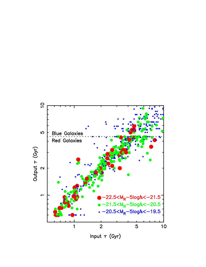
Figure 3: A comparison of the input and measured spectral types and absolute magnitudes for simulated galaxies with photometric redshifts in the range $0.30<z<0.90$. The $\tau<4.5~{}{\rm Gyr}$ selection criterion is shown with the dotted line in the left-hand panel. There is good agreement between the input and output $\tau$ and $M_{R}$ values for red galaxies. Few blue galaxies are scattered into the red galaxy sample. Some structure can be observed in the $\tau$ output values due to the interpolated models only being evaluated when their colors and redshifts differ significantly from the other models.

The conclusions of this paper rely on the accuracy of the galaxy spectral classifications and absolute magnitudes. Significant contamination by late-type spirals or $R>21$ faint blue galaxies will dramatically decrease angular and spatial two-point correlation functions (Efstathiou et al., 1991). To minimize contamination, the photometric redshift range was restricted to $0.30<z<0.90$, where the $\tau$-models are not degenerate for $B_{W}RI$ photometry. The bulk of the spectra used in Figure 1 have relatively low signal-to-noise ratios making it difficult to verify the selection criteria spectroscopically with currently available datasets. Instead, we used the simulated data and compared the values of $\tau$ and $M_{R}$ used to generate the model object with the output $\tau$ and $M_{R}$ values from the photometric redshift code. As shown in Figure 3, there is good agreement between the input and output values of $\tau$ and $M_{R}$ for red galaxies. Few blue galaxies are scattered into the red sample while a small fraction of red galaxies are scattered out of the sample. For the remainder of the paper, we restrict the magnitude range to $R\leq 23.25$, where tests with simulated galaxies indicate $\tau$ is being reliably measured. While some contamination is inevitable, it is reasonable to assume that weakly clustered faint blue galaxies (e.g., Efstathiou et al., 1991) are not dominating the measured angular correlation function. The final red galaxy sample contains 5325 objects, which is 14% of all 39316, $R\leq 23.25$ galaxies in the $1.2\Box^{\circ}$ sample area.

5 The correlation function

We determined the angular correlation function using the Landy & Szalay (1993) estimator:

$$\hat{\omega}(\theta)=\frac{DD-2DR+RR}{RR}$$ (2)

where $DD$, $DR$, and $RR$ are the number of galaxy-galaxy, galaxy-random and random-random pairs at angular separation $\theta\pm\delta\theta/2$. The pair counts were determined in logarithmically spaced bins between $10^{\prime\prime}$ and $1^{\circ}$.

The random objects consist of copies of real galaxies which have had their positions changed to mimic objects that are randomly distributed across the sky. This does not result in a perfectly uniform surface density of objects across the field due to the completeness variations in the 4 subfields. When the “random” objects were distributed across the field, the probability of each object being detected in a given subfield was estimated and the product of this and the subfield area was used when determining which subfield the object would be placed. To decrease the contribution of the random objects to the shot-noise, 100 random object catalogs were generated and $DR$ and $RR$ were renormalized accordingly.

The estimator of the correlation function is subject to the integral constraint

$$\int\int\hat{\omega}(\theta_{12})d\Omega_{1}d\Omega_{2}\simeq 0$$ (3)

(Groth & Peebles, 1977) which results in a systematic underestimate of the clustering. To remove this bias, the term

$$\omega_{\Omega}=\frac{1}{\Omega^{2}}\int\int\omega(\theta_{12})d\Omega_{1}d\Omega_{2}$$ (4)

was added to $\hat{\omega}(\theta)$ where $\Omega$ is the survey area. The value of $\bar{n}^{2}\omega_{\Omega}$, where $\bar{n}$ is the mean number of galaxies per area $\Omega$, is the contribution of clustering to the variance of the galaxy number counts (Groth & Peebles, 1977; Efstathiou et al., 1991). The angular correlation function was assumed to be a power-law given by

$$\omega(\theta)=\omega(1^{\prime})\left(\frac{\theta}{1^{\prime}}\right)^{1-\gamma}$$ (5)

where $\gamma$ is a constant. This is a good approximation of the observed spatial correlation function from the 2dFGRS and SDSS surveys on scales of $\lesssim 10h^{-1}{\rm Mpc}$ (Norberg et al., 2001; Zehavi et al., 2002). For a $\gamma=1.87$ power-law, the integral constraint for this study was approximately $6\%$ of the amplitude of the correlation function at $1^{\prime}$.

We determined the covariance matrix of $\omega(\theta)$ using the approximation of Eisenstein & Zaldarriaga (2001):

$$C_{\omega}(\theta_{i},\theta_{j})=\frac{1}{\pi\Omega^{2}}\int_{0}^{\infty}KP^{2}_{2}(K)J_{0}(K\theta_{i})J_{0}(K\theta_{j})dK$$ (6)

where $J_{0}$ is a Bessel function and $P^{2}_{2}(K)$ is the angular power spectrum,

$$P_{2}(K)=2\pi\int_{0}^{\infty}w(\theta)J_{0}(K\theta)\theta d\theta.$$ (7)

This approximation is best suited to correlation functions where $\omega(\theta)\ll 1$ and underestimates the covariance of very strongly clustered objects. For the evaluation of $P_{2}(K)$, we truncated the power-law form of the correlation function at $2^{\circ}$ as the $z\sim 0$ galaxy correlation function is $\approx 0$ on scales of $>20h^{-1}{\rm Mpc}$ (e.g., Maddox, Efstathiou, & Sutherland, 1996; Connolly et al., 2002). However, the power-law fits to the data are only marginally affected by the value of $P_{2}(K)$ on large scales. If the angular correlation function bins have significant width, Equation 6 is modified to

$$C_{\omega}(\theta_{i},\theta_{j})=\left(\frac{2}{\theta_{i,2}^{2}-\theta_{i,1}^{2}}\right)\left(\frac{2}{\theta_{j,2}^{2}-\theta_{j,1}^{2}}\right)\int^{\theta_{i,2}}_{\theta_{i,1}}\int^{\theta_{j,2}}_{\theta_{j,1}}\theta\theta^{\prime}C_{\omega}(\theta,\theta^{\prime})d\theta d\theta^{\prime}$$ (8)

(D. Eisenstein 2003, private communication) where $\theta_{1}$ and $\theta_{2}$ are the inner and outer radii of the bins. This can be rewritten as the single integral

$$C_{\omega}(\theta_{i},\theta_{j})=\frac{4}{(\theta_{i,2}^{2}-\theta_{i,1}^{2})(\theta_{j,2}^{2}-\theta_{j,1}^{2})\pi\Omega^{2}}\times$$

$$\int^{\infty}_{0}P_{2}^{2}(K)\left[\theta_{i,2}J_{1}(K\theta_{i,2})-\theta_{i,1}J_{1}(K\theta_{i,1})\right]\left[\theta_{j,2}J_{1}(K\theta_{j,2})-\theta_{j,1}J_{1}(K\theta_{j,1})\right]\frac{dK}{K}.$$ (9)

The contribution of shot noise to the estimate of the covariance was included by adding the reciprocal of the sky surface density of galaxies (per steradian) to $P_{2}(k)$. However, the shot noise only dominates the covariance on scales of $\lesssim 1^{\prime}$ for the red galaxy sample.

The spatial correlation function was obtained using Limber’s (1954) equation:

$$\omega(\theta)=\int^{\infty}_{0}\frac{dN}{dz}\left[\int^{\infty}_{0}\xi(r(\theta,z,z^{\prime}),z)\frac{dN}{dz^{\prime}}dz^{\prime}\right]dz\left/\left(\int^{\infty}_{0}\frac{dN}{dz}dz\right)^{2}\right.$$ (10)

where $\frac{dN}{dz}$ is the redshift distribution, $\xi$ is the spatial correlation function and $r(\theta,z,z^{\prime})$ is the comoving distance between two objects at redshifts $z$ and $z^{\prime}$ separated by angle $\theta$ on the sky. The spatial correlation function was assumed to be a power law given by

$$\xi(r,z)=[r/r_{0}(z)]^{-\gamma}$$ (11)

where

$$r_{0}(z)=r_{0}(0)[1+z]^{-(3+\epsilon-\gamma)/\gamma}$$ (12)

and $\epsilon$ is a constant (Groth & Peebles, 1977). Clustering is fixed in physical or comoving coordinates if $\epsilon=0$ or $\epsilon=\gamma-3$ respectively.

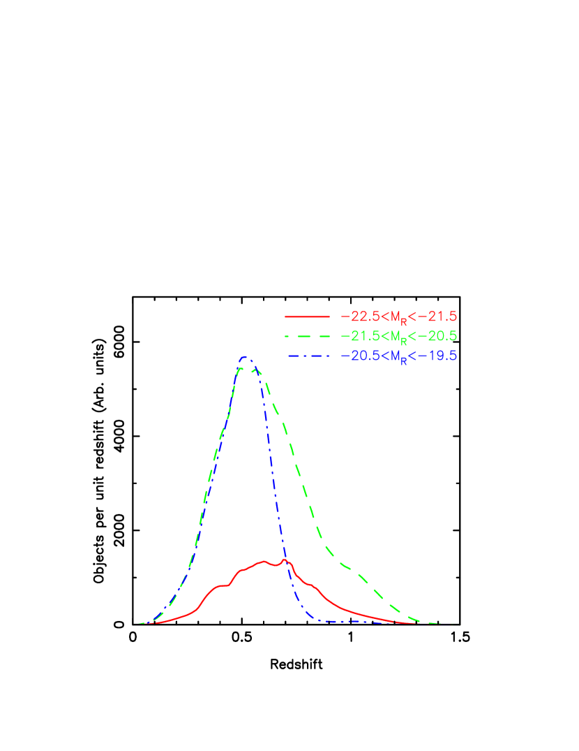
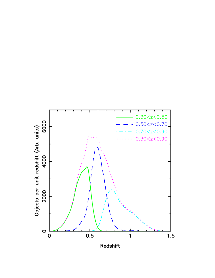
Figure 5: The redshift distributions used to evaluate the spatial correlation function of the $\tau<4.5~{}{\rm Gyr}$ samples as a function of luminosity (left panel) and redshift (right panel). The redshift distributions of adjoining photometric redshift bins have significant overlaps and the resulting estimates of $r_{0}$ for these bins cannot be considered entirely independent. The redshift distribution of the most luminous red galaxies shows evidence of individual structures in redshift space. The redshift distributions of the $\tau<2.0~{}{\rm Gyr}$ subsamples (which are not shown) have comparable shapes but different normalizations.

We estimated the redshift distribution for Limber’s equation by summing the redshift likelihood distributions of the individual galaxies in each subsample. As shown in Figure 4, the redshift distributions of individual galaxies can not be modeled with Gaussians and estimates derived from the photometric redshift code $\chi^{2}$ as a function of redshift must be used instead. Model redshift distributions for several subsamples selected by luminosity and photometric redshift are shown in Figure 5.

6 The clustering of red galaxies

6.1 The angular and spatial correlation functions

The angular correlation function was determined for red galaxies in a series of photometric redshift bins between $z=0.30$ and $z=0.90$, and absolute magnitude bins between $M_{R}-5{\rm log}h=-22.5$ and $M_{R}-5{\rm log}h=-19.5$. All bins are volume limited samples containing galaxies brighter than $R=23.25$. A power-law of the form $\omega(\theta)=\omega(1^{\prime})(\theta/1^{\prime})^{1-\gamma}$ was fitted to the $\theta<0.25^{\circ}$ data with $\gamma$ fixed to $1.87$, the value for $z<0.15$ early-type galaxies (Norberg et al., 2002; Zehavi et al., 2002). We use $\omega(1^{\prime})$ rather than $\omega(1^{\circ})$ for the power-law fits as it depends less on the assumed value of $\gamma$. The amplitude of the two-point angular correlation functions for these subsamples are summarized in Tables 2 and 3. Angular correlation functions for $-21.5<M_{R}-5{\rm log}h<20.5$, $\tau<4.5~{}{\rm Gyr}$ galaxies are also plotted in Figure 6.

A summary of the spatial clustering (parameterized by $r_{0}$) as a function of spectral type, absolute magnitude, and redshift is presented in Tables 2 and 3. The estimates of $r_{0}$ in the narrow redshift bins are consistent with the values in the widest redshift bins. While this is expected, it is not always the case as the largest redshift bin contains object pairs which are not present in the smallest bin. The width of the redshift distribution for the smallest bin strongly depends on the uncertainties of the photometric redshifts as these uncertainties are comparable to the bin width. In contrast, the shape of the redshift distribution of the largest bin depends mostly on the bin width as the uncertainties of the photometric redshifts are smaller than the width of the bin. If the uncertainties are systematically underestimated, Limber’s equation will overestimate the number of close object pairs in the narrowest bin and underestimate the value of $r_{0}$. If the uncertainties in the redshift distribution were not included, $r_{0}$ would vary between $3.9\pm 0.4h^{-1}{\rm Mpc}$ and $5.5\pm 0.4h^{-1}{\rm Mpc}$ for the narrowest and widest redshift bins for $-21.0<M_{R}-5{\rm log}h<-20.0$, $\tau<4.5~{}{\rm Gyr}$ galaxies. The measured evolution of $r_{0}$ should be independent of the width of the redshift bins and confirming this is an extremely useful internal consistency check which should always be applied to correlation functions using photometric redshifts.

6.2 Clustering as a function of absolute magnitude

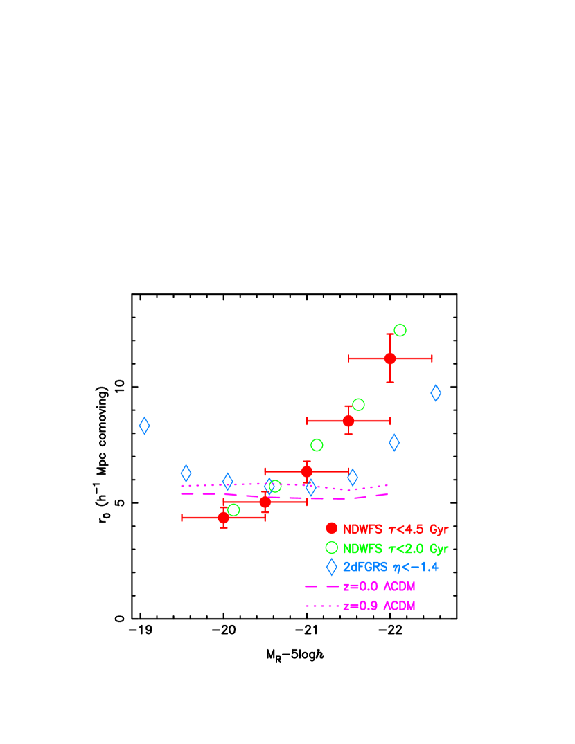
Figure 7: The spatial clustering of red galaxies as a function of absolute magnitude. For clarity, only the uncertainties for the $\tau<4.5~{}{\rm Gyr}$ data are shown and the $\tau<2.0~{}{\rm Gyr}$ data has been shifted slightly to the right. While datapoints brighter than $M_{R}-5{\rm log}h=-20.5$ include galaxies over the entire $0.30<z<0.90$ photometric redshift range, fainter bins have a truncated redshift range. The $z<0.15$ 2dFGRS data points, which have uncertainties of $\sim 0.5h^{-1}{\rm Mpc}$, are over-plotted using the assumption that $B_{J}-R=1.25$ for red galaxies. The clustering of red galaxies is a strong function of luminosity and a weaker function of spectral type. A $\Lambda$CDM simulation of the clustering $B-R>1.24$ galaxies (Benson et al., 2001, A. Benson 2002, private communication) reproduces the clustering of $L^{*}$ galaxies but the $141^{3}h^{-3}{\rm Mpc^{3}}$ simulation volume is insufficient to measure the clustering of luminous galaxies.

Figure 7 and Table 2 present estimates of the spatial clustering of red galaxies as a function of evolution corrected absolute magnitude. Absolute magnitude bins containing galaxies brighter than $M_{R}-5{\rm log}h=-20.5$ include the entire $0.30<z<0.90$ photometric redshift range while fainter bins have truncated redshift ranges which are listed in Table 2. While redder galaxies are more strongly clustered than bluer galaxies, the striking correlation is between $r_{0}$ and absolute magnitude. While there is a mild correlation with luminosity at $M_{R}-5{\rm log}h\sim-20.0$, the value of $r_{0}$ rapidly increases from $r_{0}=6.3h^{-1}{\rm Mpc}$ at $M_{R}-5{\rm log}h=-21$ to $r_{0}=11.2h^{-1}{\rm Mpc}$ at $M_{R}-5{\rm log}h=-22$. Similar behavior is seen for at $z<0.15$ in the SSRS2 and 2dFGRS (Willmer, da Costa, & Pellegrini, 1998; Norberg et al., 2002), and, with lower significance, in CNOC2 at $z<0.4$ (Shepherd et al., 2001). Hogg et al. (2003) observe similar trends in the SDSS at $0.05<z<0.22$ by measuring density of galaxy neighbors within $8h^{-1}{\rm Mpc}$ spheres as a function of galaxy color and luminosity. Wilson (2003) measures $r_{0}=4.02\pm 0.22h^{-1}{\rm Mpc}$ for $0.2<z<1.0$, $M_{B}<-18.61$ red galaxies, but her model redshift distribution does not include the uncertainties of her $V-I$ photometric redshifts, so her value of $r_{0}$ is a lower limit. A summary of previous measurements of red galaxy correlation functions is provided in Table 4.

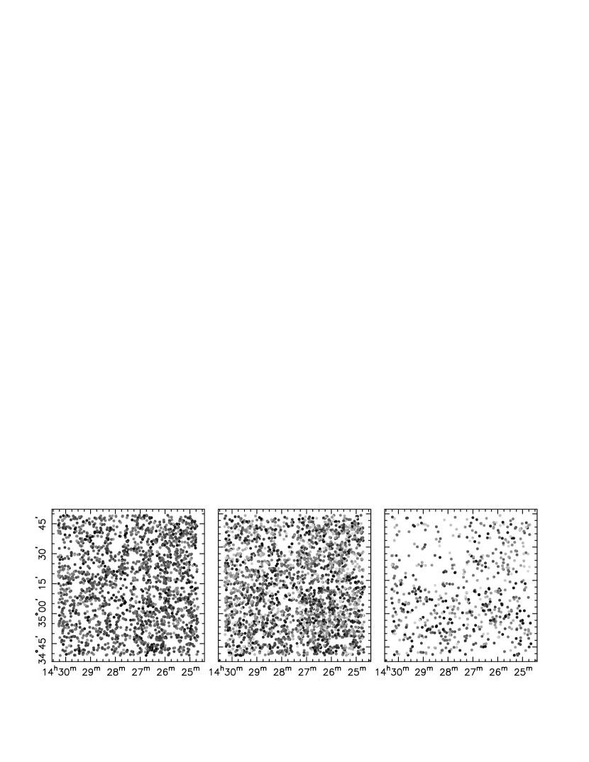
Figure 8: The distribution of red galaxies on the plane of the sky for several absolute magnitude bins. The bins are (from left to right) $-20.5<M_{R}-5{\rm log}h<-19.5$, $-21.5<M_{R}-5{\rm log}h<-20.5$ and $-22.5<M_{R}-5{\rm log}h<-21.5$. The greyscale of the dots is related to the photometric redshift, with dark dots at low redshift and light dots at high redshift. Rectangular voids in the galaxy distribution are the boundaries between the NDWFS subfields and regions surrounding bright stars. The distribution of luminous galaxies clearly shows evidence for structures comparable to the area of the subfields, suggesting that surveys of this size are susceptible to cosmic variance.

While the $r_{0}$ values of $M_{R}-5{\rm log}h>-21.5$ galaxies from the NDWFS and 2dFGRS show only marginal differences, the $r_{0}$ values of luminous galaxies in the NDWFS are higher than those of the 2dFGRS with $\approx 2\sigma$ significance. Clustering evolution would be expected to produce decreasing $r_{0}$ values with increasing redshift rather than the opposite trend seen in Figure 7. However, as luminous galaxies are more strongly clustered than $L^{*}$ galaxies, estimates of their clustering are also more susceptible to cosmic variance. The distribution of galaxies on the plane of the sky, which is plotted in Figure 8, clearly shows that luminous galaxies are in structures comparable in size to the field-of-view. While it is plausible that selection effects could produce the observed structures, stars selected with the same selection criteria do not show similar large-scale structure. In addition, in Figure 5, the model redshift distribution of the most luminous red galaxies shows evidence of individual structures. We therefore assume that the $2\sigma$ difference between the clustering of luminous galaxies in the NDWFS and 2dFGRS is due cosmic variance. Even if cosmic variance were not an issue, it is difficult to measure clustering evolution with galaxies in the absolute magnitude range where $r_{0}$ is strongly correlated with luminosity as small luminosity errors can translate into large errors in $r_{0}$. It is therefore preferable to measure clustering evolution with $M_{R}-5{\rm log}h>-21.5$ galaxies, as we have done in §6.3.

As the correlation between $r_{0}$ and spectral type is relatively weak in the NDWFS and 2dFGRS, our measurements of the evolution of clustering are not sensitive to small errors in the estimates of the spectral types. The strong correlation between $r_{0}$ and absolute magnitude for luminous galaxies is a prediction of recent large volume $\Lambda$CDM simulations (e.g., Benson et al., 2001). As shown in Figure 7, a $141^{3}h^{-3}{\rm Mpc^{3}}$ $\Lambda$CDM simulation with galaxy selection criteria similar to the $\tau<4.5~{}{\rm Gyr}$ sample (Benson et al., 2001, A. Benson 2002, private communication) is a good approximation of the clustering of $M_{R}\sim-21$ red galaxies.

6.3 Evolution of the spatial correlation function

The evolution of spatial clustering galaxies was studied with $-21.5<M_{R}-5{\rm log}h<-20.5$ red galaxies. Luminous galaxies were excluded as their spatial clustering is strongly correlated with absolute magnitude and small redshift or spectral evolution errors could produce large changes in the measured spatial clustering. The faint limit was chosen to allow the same range of absolute magnitudes to be studied over a broad redshift range.

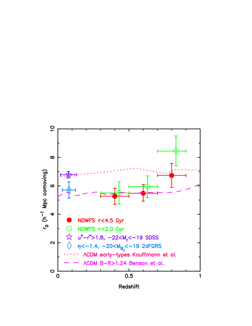
Figure 9: The spatial correlation function parameter $r_{0}$ as a function of redshift for the NDWFS, 2dFGRS, and SDSS red galaxy samples. For clarity, the $\tau<2.0~{}{\rm Gyr}$ data points have been shifted slightly to the right. The horizontal bars indicate the photometric (NDWFS) and spectroscopic (2dFGRS, SDSS) redshift ranges. The clustering of $\tau<4.5~{}{\rm Gyr}$ galaxies (which were selected to allow direct comparison with the 2dFGRS) is well approximated by $\Lambda$CDM simulations of the clustering of early-type and $B-R>1.24$ galaxies (Kauffmann et al., 1999; Benson et al., 2001, A. Benson 2002, private communication). From the plot, it is clear the value of $r_{0}$ (in comoving coordinates) undergoes little or no evolution over the redshift range observed.

As shown in Figure 9 and Table 3, no significant evolution of $r_{0}$ (comoving) occurs over the redshift range studied. Two models of the clustering of red galaxies, derived from the GIF $\Lambda$CDM simulations (Jenkins et al., 1998), are plotted in Figure 9 and provide good approximations to the measured clustering from the NDWFS, SDSS and 2dFGRS. The Kauffmann et al. (1999) model predicts the clustering of early-type galaxies with stellar masses of $>3\times 10^{10}M_{\sun}$ while the Benson (2002, private communication) simulation models the clustering of $B-R>1.24$, $-20.5<M_{R}-5{\rm log}h<-21.5$ galaxies. If the evolution of the underlying dark matter distribution at $z<1$ is well described by the linear or quasi-linear growth of density perturbations, the bias of red galaxies must be rapidly evolving with redshift.

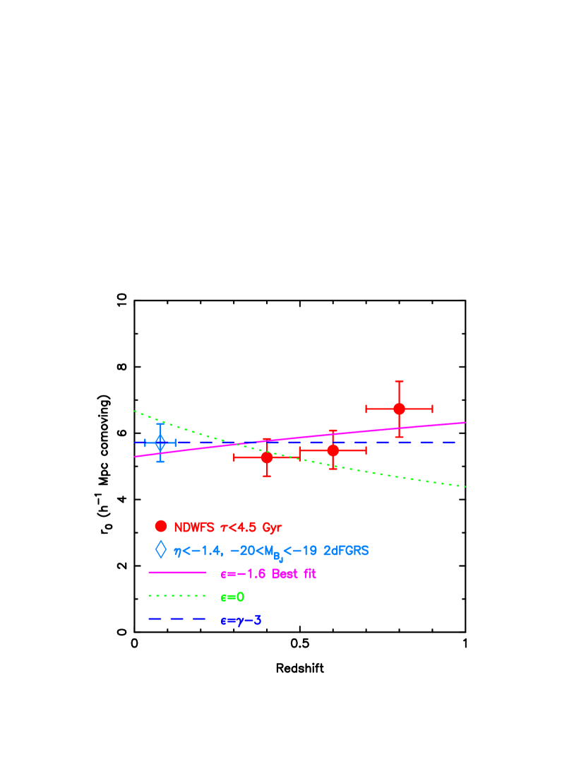
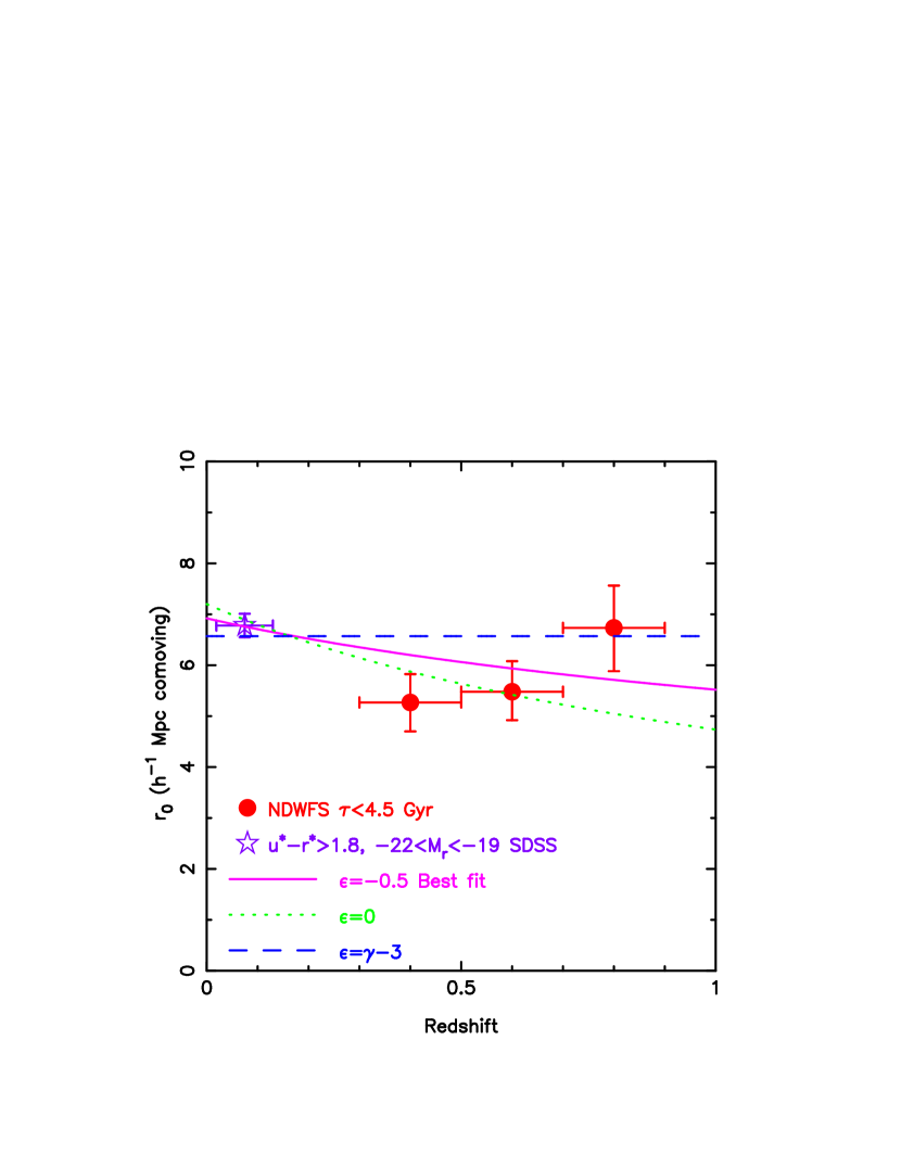
Figure 10: The evolution of $r_{0}$ (comoving). The NDWFS data are shown with the comparable low redshift data from the 2dFGRS (left panel) and SDSS (right panel). Models with clustering fixed in physical coordinates ($\epsilon=0$) are rejected with $2.5\sigma$ confidence by the NDWFS and 2dFGRS while models with little or no evolution ($\epsilon\simeq\gamma-3$) provide acceptable fits to the observed clustering.

The evolution of $r_{0}$ was empirically measured by estimating the clustering evolution parameter $\epsilon$ (from Equation 12). The $0.30<z<0.50$ and $0.70<z<0.90$ bins were assumed to be independent estimates of $r_{0}$ at the median redshifts of their model redshift distributions. The 2dFGRS and SDSS clustering estimates were also included to provide additional constraints on $\epsilon$. The selection criteria for the NDWFS $\tau<4.5~{}{\rm Gyr}$ sample allow direct comparison with the 2dFGRS early-type sample of Norberg et al. (2002). The present-day colors of the NDWFS $\tau<4.5~{}{\rm Gyr}$ sample are only $\simeq 0.15$ magnitudes redder in $B_{W}-R$ than the SDSS $u^{*}-r^{*}>1.8$ sample of Zehavi et al. (2002). The best-fit estimates of $\epsilon$ are summarized in Table 5 and plotted in Figure 10. Models with $\epsilon=0$ are rejected with $>2.5\sigma$ confidence when constraints from the 2dFGRS are included with the NDWFS data. The evolution of $r_{0}$ is consistent with clustering fixed in comoving coordinates ($\epsilon=\gamma-3$) at $z<0.90$.

7 Discussion

The clustering of red galaxies undergoes little or no evolution from $z\sim 0.9$ to the present-day. At $z>0.9$, the only published clustering study using comparable template selection criteria is that of Firth et al. (2002) which used galaxies fitted with the evolving E and Sbc templates of the HYPERZ photometric redshift code (Bolzonella, Miralles & Pelló, 2000). Their estimate of $r_{0}=7.0\pm 1.9h^{-1}{\rm Mpc}$, with $\gamma$ assumed to be $1.8$, is consistent with $r_{0}$ remaining fixed in comoving coordinates to $z\approx 1.5$. However, to differentiate between currently plausible $\Lambda$CDM models larger survey areas, on the order of the complete NDWFS ($\approx 18\Box^{\circ}$), will be required.

Further constraints on the clustering of $1<z<2$ galaxies are available from samples of QSOs (Croom et al., 2001) and $R-K>5$ extremely red objects (EROs; Daddi et al., 2001; Firth et al., 2002; Roche et al., 2002). The QSO spatial correlation function, measured in redshift space ($s_{0}$ replacing $r_{0}$), marginally increases from $s_{0}=5.28\pm^{0.72}_{0.89}h^{-1}{\rm Mpc}$ with $\gamma=1.72\pm^{0.23}_{0.22}$ at $z<0.95$ to $s_{0}=6.93\pm^{1.32}_{1.64}h^{-1}{\rm Mpc}$ with $\gamma=1.64\pm^{0.29}_{0.27}$ at $2.10<z<2.90$ (Croom et al., 2001). However, as pointed out by Croom et al. (2001), interpretation of QSO clustering relies on poorly constrained models of QSOs lifetimes and host populations as a function of redshift.

EROs are easier to relate to low redshift populations than QSOs as the majority appear to be the progenitors of early-type galaxies with the remainder being dusty starbursts (Dey et al., 1999; Liu et al., 2000; Moriondo et al., 2000). EROs could therefore extend the redshift range of early-type spatial correlation function evolution estimates to $z\approx 1.5$. With the exception of $H<20.5$ EROs in the Las Campanas Infrared Survey (Firth et al., 2002), all EROs clustering studies measure $r_{0}\geq 10h^{-1}{\rm Mpc}$ (Daddi et al., 2001; Firth et al., 2002; Roche et al., 2002). This is comparable to the clustering of the most luminous red and early-type galaxies at $z<1$.

If $K>19$ EROs correspond to $\lesssim L^{*}$ galaxies (Daddi et al., 2001; Roche et al., 2002), the ERO clustering results are difficult to reconcile with $z<1$ studies and $\Lambda$CDM theory. The clustering of red $L^{*}$ galaxies in the NDWFS can be increased to $r_{0}\sim 9h^{-1}{\rm Mpc}$ only by increasing the photometric redshift $1\sigma$ uncertainties to $\sim 40\%$ of the photometric redshifts or increasing the stellar contamination to $\sim 40\%$. These scenarios are inconsistent with the redshift comparisons in Figure 1 and the lack of a stellar locus in Figure 2. The discrepancy between the ERO $r_{0}$ values and $z<1$ studies could be due to errors in the ERO model redshift distributions used to deproject the angular correlation function. Firth et al. (2002), who measure $r_{0}=7.7\pm 2.4h^{-1}{\rm Mpc}$ for $H<20.5$ EROs, have few $z\gtrsim 1.5$ objects while the Daddi et al. (2001) and Roche et al. (2002) models have a significant fraction of EROs at $z\approx 2$. Improved constraints on ERO clustering should be provided with model redshift distributions constrained with photometric redshifts which have been verified with spectroscopic samples. The clustering of EROs, as measured from the NDWFS, will be described in a future paper (Brown et al., in preparation) using a $B_{W}RIK$ dataset.

8 Summary

We have used the NOAO Deep Wide-Field Survey to measure the clustering of $0.30\lesssim z\lesssim 0.90$ red galaxies. The wide-field and $B_{W}RI$ bands allow large galaxy samples to be selected as a function of spectral type and absolute magnitude using photometric redshifts. PEGASE2 spectral evolution models with exponentially decreasing star formation rates have been used to select an evolutionary sequence of related galaxies as a function of redshift. The red sample, with present-day rest-frame colors of $B_{W}-R>1.44$, was chosen to allow direct comparison with the low redshift early-type sample from the 2dFGRS. The clustering of red galaxies is strongly correlated with luminosity, with $r_{0}$ increasing from $4.4\pm 0.4h^{-1}{\rm Mpc}$ at $M_{R}-5{\rm log}h\approx-20.0$ to $11.2\pm 1.0h^{-1}{\rm Mpc}$ at $M_{R}-5{\rm log}h\approx-22.0$. Clustering evolution measurements with samples where the distribution of spectral types and luminosities are a function of redshift will be dominated by selection effects. The strength of $r_{0}$ (comoving) as a function of absolute magnitude in our sample is comparable to estimates at $z<0.15$ from the 2dFGRS, with differences at high luminosity being attributable to structures of sizes comparable to the field-of-view. No significant evolution of $r_{0}$ was detected in comparisons of the NDWFS with the 2dFGRS and SDSS. For $0.30<z<0.90$, $-21.5<M_{R}-5{\rm log}h<-20.5$, $B_{W}-R>1.44$ galaxies, the largest sample studied, the value of $r_{0}$ is $6.3\pm 0.5h^{-1}{\rm Mpc}$ with $\gamma$ fixed at $1.87$. The strong clustering and lack of detectable evolution appears consistent with recent $\Lambda$CDM models where the bias undergoes rapid evolution and $r_{0}$ undergoes little evolution at $z<2$.

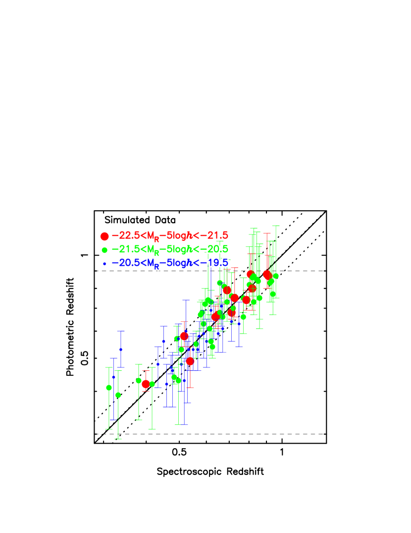
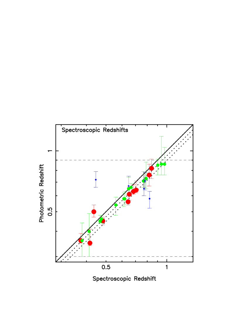
Figure 1: A comparison of the photometric and spectroscopic redshifts of $-22.5<M_{R}-5{\rm log}h<-19.5$ red galaxies ($\tau<4.5~{}{\rm Gyr}$) with photometric redshifts in the range $0.30<z<0.90$. Dashed horizontal lines mark the upper and lower limits of the photometric redshift range. Dotted diagonal lines show the median offset and $\pm 1\sigma$ uncertainty of the photometric redshifts. Simulated galaxies, generated using the $\tau$-models with photometric noise added, are shown in the lefthand panel. On the right are real galaxies with spectroscopic redshifts from the NED database and unpublished spectra. The real galaxies show a $5\%$ systematic offset between the photometric and spectroscopic redshifts. With the inclusion of 0.05 magnitudes of intrinsic scatter, the real data have $1\sigma$ uncertainty estimates which are consistent with the measured scatter between the photometric and spectroscopic redshifts.

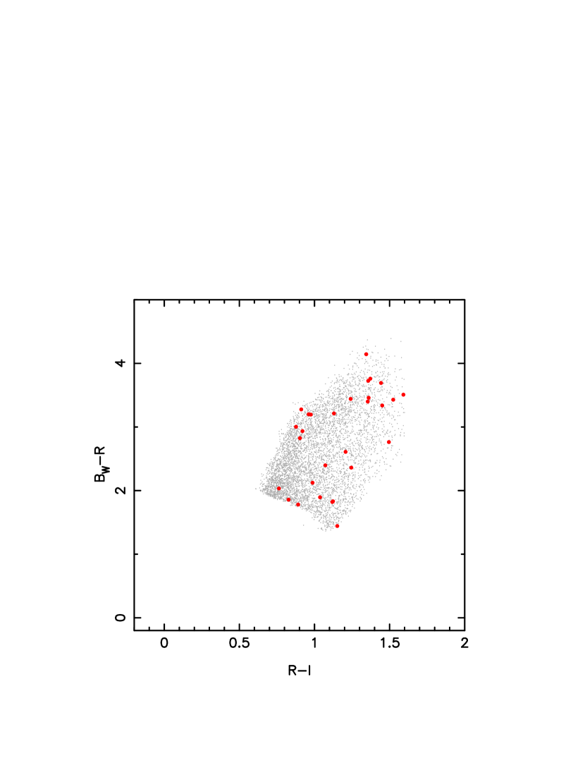
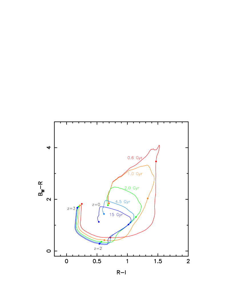
Figure 2: The Vega colors of the $\tau<4.5~{}{\rm Gyr}$, $0.30<z<0.90$ NDWFS Boötes galaxy sample (left panel) and the $\tau$-models (right panel). Bold points in the left hand panel show the colors of galaxies with spectroscopic redshifts (including Cetus and Lockman Hole galaxies) which were used to test the accuracy of the photometric redshifts. Bold points on the model tracks mark the predicted colors of $z=0$, 1, 2 and 3 galaxies for each of the models. For clarity, only five of the $\tau$-model tracks are plotted. The $\tau$-models occupy the same region of color space as the NDWFS red galaxies. Single burst models (not shown) have different colors as a function of redshift. A more detailed description of the colors of NDWFS galaxies and the accuracy of galaxy stellar evolution models will be provided by Dey et al. (in preparation).

Figure 4: The redshift likelihood distribution produced by the photometric redshift code. ${\rm NDWFS~{}J142518.9+353545}$, which has a spectroscopic redshift of 0.705, has a photometric redshift of 0.63 (shown by the arrow) and a spectral type of $\tau=0.64~{}{\rm Gyr}$. Unlike Brunner et al. (2000) and Brown, Boyle & Webster (2001), we can not adequately model the redshift likelihood distribution with a Gaussian.

Figure 6: The angular correlation functions of $\tau<4.5~{}{\rm Gyr}$, $-21.5<M_{R}-5{\rm log}h<-20.5$ galaxies selected from the NDWFS. The first three panels show the angular correlation functions for the narrowest photometric redshift bins while the last panel shows the angular correlation function for the $0.30<z<0.90$ bin. On small angular scales shot noise dominates the uncertainties while on larger scales the contribution of clustering to the covariance dominates. Power-law fits to the data are shown along with $\pm 1\sigma$ errors (dotted lines). For reference, $0.1^{\circ}$ corresponds to a transverse comoving distance of $3h^{-1}{\rm Mpc}$ at $z\approx 0.7$.

Table 1: The four subfields of the first NDWFS public data release.

Subfield name	R.A.	Decl.	Delivered FWHM (′′)			Integration time(hours)			50% completeness limit
	(J2000.0)	(J2000.0)	$B_{W}$	$R$	$I$	$B_{W}$	$R$	$I$	$B_{W}$	$R$	$I$
NDWFS J1426+3531	14 26 00.8	+35 31 32	1.2	1.6	1.3	2.1	1.7	3.0	26.8	24.8	24.7
NDWFS J1426+3456	14 26 01.4	+34 56 32	1.3	1.2	1.0	2.3	1.2	2.1	26.5	25.3	24.9
NDWFS J1428+3531	14 28 52.8	+35 31 39	1.5	1.3	0.7	2.3	1.7	2.2	26.4	25.0	25.6
NDWFS J1428+3456	14 28 52.2	+34 56 39	1.6	1.3	1.3	2.3	1.7	2.6	26.2	25.0	23.6

Table 2: The correlation function of red galaxies in the NDWFS as a function of absolute magnitude.

Selection	Photo. $z$ range	Absolute magnitude	Apparent magnitude	Galaxies	Contamination	$\omega(1^{\prime})$	Median $z$	$r_{0}(h^{-1}{\rm Mpc})$
$\tau<4.5~{}{\rm Gyr}$	0.30-0.90	$-22.50<M_{R}<-21.50$	$18.18\leq R\leq 22.43$	660	0.009	$0.41\pm 0.07$	0.64	$11.2\pm 1.0$
$\tau<4.5~{}{\rm Gyr}$	0.30-0.90	$-22.00<M_{R}<-21.00$	$18.30\leq R\leq 23.01$	1677	0.005	$0.24\pm 0.03$	0.61	$8.5\pm 0.6$
$\tau<4.5~{}{\rm Gyr}$	0.30-0.90	$-21.50<M_{R}<-20.50$	$18.76\leq R\leq 23.25$	2651	0.023	$0.14\pm 0.02$	0.60	$6.3\pm 0.5$
$\tau<4.5~{}{\rm Gyr}$	0.30-0.75	$-21.00<M_{R}<-20.00$	$19.17\leq R\leq 23.17$	2429	0.009	$0.12\pm 0.02$	0.55	$5.0\pm 0.4$
$\tau<4.5~{}{\rm Gyr}$	0.30-0.65	$-20.50<M_{R}<-19.50$	$19.72\leq R\leq 23.08$	1756	0.025	$0.12\pm 0.02$	0.51	$4.4\pm 0.4$
$\tau<2.0~{}{\rm Gyr}$	0.30-0.90	$-22.50<M_{R}<-21.50$	$18.18\leq R\leq 22.43$	488	0.011	$0.52\pm 0.10$	0.66	$12.4\pm 1.2$
$\tau<2.0~{}{\rm Gyr}$	0.30-0.90	$-22.00<M_{R}<-21.00$	$18.30\leq R\leq 23.01$	1122	0.006	$0.29\pm 0.05$	0.64	$9.2\pm 0.8$
$\tau<2.0~{}{\rm Gyr}$	0.30-0.90	$-21.50<M_{R}<-20.50$	$18.76\leq R\leq 23.25$	1592	0.037	$0.20\pm 0.03$	0.62	$7.5\pm 0.6$
$\tau<2.0~{}{\rm Gyr}$	0.30-0.75	$-21.00<M_{R}<-20.00$	$19.25\leq R\leq 23.17$	1337	0.016	$0.16\pm 0.04$	0.57	$5.7\pm 0.7$
$\tau<2.0~{}{\rm Gyr}$	0.30-0.65	$-20.50<M_{R}<-19.50$	$19.87\leq R\leq 23.08$	929	0.043	$0.14\pm 0.04$	0.53	$4.7\pm 0.7$

Table 3: The correlation function of red galaxies in the NDWFS as a function of photometric redshift.

Selection	Photo. $z$ range	Absolute magnitude	Apparent magnitude	Galaxies	Contamination	$\omega(1^{\prime})$	Median $z$	$r_{0}(h^{-1}{\rm Mpc})$
$\tau<4.5~{}{\rm Gyr}$	0.30-0.50	$-21.50<M_{R}<-20.50$	$18.76\leq R\leq 21.25$	853	0.003	$0.25\pm 0.05$	0.42	$5.3\pm 0.6$
$\tau<4.5~{}{\rm Gyr}$	0.50-0.70	$-21.50<M_{R}<-20.50$	$20.05\leq R\leq 22.50$	1023	0.002	$0.24\pm 0.05$	0.60	$5.5\pm 0.6$
$\tau<4.5~{}{\rm Gyr}$	0.70-0.90	$-21.50<M_{R}<-20.50$	$20.99\leq R\leq 23.25$	775	0.071	$0.20\pm 0.05$	0.85	$6.7\pm 0.8$
$\tau<4.5~{}{\rm Gyr}$	0.30-0.70	$-21.50<M_{R}<-20.50$	$18.76\leq R\leq 22.50$	1876	0.003	$0.19\pm 0.03$	0.52	$5.9\pm 0.5$
$\tau<4.5~{}{\rm Gyr}$	0.50-0.90	$-21.50<M_{R}<-20.50$	$20.05\leq R\leq 23.25$	1798	0.032	$0.17\pm 0.03$	0.69	$6.3\pm 0.5$
$\tau<4.5~{}{\rm Gyr}$	0.30-0.90	$-21.50<M_{R}<-20.50$	$18.76\leq R\leq 23.25$	2651	0.023	$0.14\pm 0.02$	0.60	$6.3\pm 0.5$
$\tau<2.0~{}{\rm Gyr}$	0.30-0.50	$-21.50<M_{R}<-20.50$	$18.76\leq R\leq 21.25$	435	0.005	$0.31\pm 0.08$	0.44	$5.5\pm 0.8$
$\tau<2.0~{}{\rm Gyr}$	0.50-0.70	$-21.50<M_{R}<-20.50$	$20.12\leq R\leq 22.50$	665	0.004	$0.29\pm 0.07$	0.61	$5.9\pm 0.8$
$\tau<2.0~{}{\rm Gyr}$	0.70-0.90	$-21.50<M_{R}<-20.50$	$21.20\leq R\leq 23.25$	492	0.111	$0.31\pm 0.07$	0.85	$8.4\pm 1.0$
$\tau<2.0~{}{\rm Gyr}$	0.30-0.70	$-21.50<M_{R}<-20.50$	$18.76\leq R\leq 22.50$	1100	0.004	$0.20\pm 0.04$	0.55	$5.8\pm 0.7$
$\tau<2.0~{}{\rm Gyr}$	0.50-0.90	$-21.50<M_{R}<-20.50$	$20.12\leq R\leq 23.25$	1157	0.050	$0.22\pm 0.04$	0.69	$7.1\pm 0.7$
$\tau<2.0~{}{\rm Gyr}$	0.30-0.90	$-21.50<M_{R}<-20.50$	$18.76\leq R\leq 23.25$	1592	0.037	$0.20\pm 0.03$	0.62	$7.5\pm 0.6$

Table 4: A summary of several studies of early-type and red galaxy correlation functions.

Survey	Redshift Range	Galaxies	Magnitude Range	Selection	$r_{0}(h^{-1}{\rm Mpc~{}comoving})$	$\gamma$
NDWFS	$0.30<z<0.90$	2651	$-21.5<M_{R}<-20.5$	$\tau<4.5~{}{\rm Gyr}$	$6.3\pm 0.5$	$1.87$
NDWFS	$0.30<z<0.90$	1592	$-21.5<M_{R}<-20.5$	$\tau<2.0~{}{\rm Gyr}$	$7.5\pm 0.6$	$1.87$
Perseus-Pisces	$z\leq 0.04$	278	$M_{Z_{W}}<-19.5$	Morphology	$8.35\pm 0.75$	$2.05^{+0.10}_{-0.08}$
SSRS2	$z\leq 0.020$	395	$M_{B}<-19.4$	Morphology	$5.10\pm 0.38$	$1.91\pm 0.26$
SSRS2	$z\leq 0.027$	418	$M_{B}<-20.0$	Morphology	$5.27\pm 0.46$	$1.86\pm 0.29$
SSRS2	$z\leq 0.033$	372	$M_{B}<-20.5$	Morphology	$5.73\pm 0.56$	$2.30\pm 0.46$
SSRS2	$z\leq 0.040$	272	$M_{B}<-20.9$	Morphology	$8.60\pm 1.44$	$2.45\pm 0.71$
APM	$z\lesssim 0.1$	336	$-22<M_{B_{J}}<-15$	Morphology	$5.9\pm 0.7$	$1.85\pm 0.13$
2dFGRS	$0.016\leq z\leq 0.071$	1909	$-18.5<M_{B_{J}}<-17.5$	Red SED ($\eta<-1.4$)	$8.33\pm 1.82$	$1.87\pm 0.23$
2dFGRS	$0.020\leq z\leq 0.086$	3717	$-19.0<M_{B_{J}}<-18.0$	Red SED ($\eta<-1.4$)	$6.28\pm 1.46$	$1.98\pm 0.11$
2dFGRS	$0.031\leq z\leq 0.125$	10,135	$-20.0<M_{B_{J}}<-19.0$	Red SED ($\eta<-1.4$)	$5.71\pm 0.57$	$1.87\pm 0.09$
2dFGRS	$0.048\leq z\leq 0.150$	6434	$-21.0<M_{B_{J}}<-20.0$	Red SED ($\eta<-1.4$)	$6.10\pm 0.72$	$1.80\pm 0.12$
2dFGRS	$0.072\leq z\leq 0.150$	686	$-22.0<M_{B_{J}}<-21.0$	Red SED ($\eta<-1.4$)	$9.74\pm 1.16$	$1.95\pm 0.37$
SDSS	$0.019\leq z\leq 0.13$	19,603	$14.5<r^{*}<17.6$	Rest-frame $u^{*}-r^{*}>1.8$	$6.78\pm 0.23$	$1.86\pm 0.03$
PDF	$z\lesssim 0.5$	22,359	$B_{J}<22.5$	Redder than CWW Sbc	$6.0\pm 0.3$	1.9
K20	$0.5\lesssim z\lesssim 2.0$	400	$K<19.2$	$R-K>5$	$12\pm 3$	1.8
CNOC2	$0.120<z<0.270$	248	$R_{C}<21.5$, $M_{R}<-20$	Red CWW templates	$5.35\pm 0.20$	$2.05\pm 0.08$
CNOC2	$0.270<z<0.382$	234	$R_{C}<21.5$, $M_{R}<-20$	Red CWW templates	$6.55\pm 1.16$	$2.05\pm 0.08$
CNOC2	$0.382<z<0.510$	238	$R_{C}<21.5$, $M_{R}<-20$	Red CWW templates	$6.99\pm 0.57$	$2.10\pm 0.11$
CNOC2	$0.12<z<0.40$	254	$-20.00<M_{R}<-19.25$	Red CWW templates	$5.82\pm 0.81$	$1.85\pm 0.08$
CNOC2	$0.12<z<0.40$	276	$-20.65<M_{R}<-20.00$	Red CWW templates	$5.40\pm 0.19$	$1.89\pm 0.06$
CNOC2	$0.12<z<0.40$	278	$-22.52<M_{R}<-20.65$	Red CWW templates	$6.71\pm 0.53$	$2.14\pm 0.02$
UH8K	$0.20<z<0.90$	3382	$M_{B}\lesssim-18.61$	Redder than CWW Sbc	$4.02\pm 0.22$	1.8
LCIRS	$0.3\lesssim z\lesssim 0.8$	272	$H<20.5$	Evolving E & Sbc	$7.0\pm 1.6$	1.8
LCIRS	$0.8\lesssim z\lesssim 1.5$	355	$H<20.5$	Evolving E & Sbc	$7.0\pm 1.9$	1.8
LCIRS	$0.7\lesssim z\lesssim 1.5$	337	$H<20.0$	$R-H>4$	$11.1\pm 2.0$	1.8
LCIRS	$0.7\lesssim z\lesssim 1.5$	312	$H<20.5$	$R-H>4$	$7.7\pm 2.4$	1.8
ELAIS N2	$0.5\lesssim z\lesssim 2.0$	166	$K<21.0$	$R-K>5$	10-13	1.8

Table 5: Constraints on $\epsilon$ (as defined in Equation 12) provided by the NDWFS, SDSS, and 2dFGRS.

NDWFS Sample	$z<0.2$ Sample	$r_{0}(0)(h^{-1}{\rm Mpc~{}comoving})$	$\epsilon$
$\tau<2.0~{}{\rm Gyr}$	none	$3.1\pm_{1.0}^{1.3}$	$-4.2\pm_{1.3}^{1.3}$
$\tau<4.5~{}{\rm Gyr}$	none	$3.8\pm_{1.0}^{1.3}$	$-2.9\pm_{1.1}^{1.2}$
$\tau<4.5~{}{\rm Gyr}$	SDSS $u^{*}-r^{*}>1.8$, $-22.0<M_{r^{*}}<-19.0$	$6.9\pm_{0.3}^{0.3}$	$-0.5\pm_{0.4}^{0.5}$
$\tau<4.5~{}{\rm Gyr}$	2dFGRS $\eta<-1.4$, $-20.0<M_{B_{J}}<-19.0$	$5.3\pm_{0.6}^{0.7}$	$-1.6\pm_{0.6}^{0.6}$

References

- Benson et al. (2001) Benson, A. J., Frenk, C. S., Baugh, C. M., Cole, S., & Lacey, C. G., 2001, MNRAS, 327, 1041
- Benítez (2000) Benítez, N. 2000, ApJ, 536, 571
- Bertin & Arnouts (1996) Bertin, E., & Arnouts, S. 1996, A&AS, 117, 393
- Bolzonella, Miralles & Pelló (2000) Bolzonella, M., Miralles, J.-M., & Pelló, R., 2000, A&A, 363, 476
- Brown, Boyle & Webster (2001) Brown, M. J. I., Boyle, B. J., & Webster, R. L., 2001, AJ, 122, 26
- Brunner et al. (2000) Brunner, R. J., Szalay, A. S., & Connolly, A. J., 2000, ApJ, 541, 527
- Bruzual & Charlot (1993) Bruzual, A. G., & Charlot, S. 1993, ApJ, 405, 538
- Castelli & Kurucz (1994) Castelli, F. & Kurucz, R. L. 1994, A&A, 281, 817
- Cole & Kaiser (1989) Cole, S. & Kaiser, N. 1989, MNRAS, 237, 1127
- Coleman, Wu & Weedman (1980) Coleman, G. D., Wu, C.-C., & Weedman, D. W., 1980, ApJS, 43, 393
- Connolly et al. (2002) Connolly, A. J. et al. 2002, ApJ, 579, 42
- Croom et al. (2001) Croom, S. M., Shanks, T., Boyle, B. J., Smith, R. J., Miller, L., Loaring, N. S., & Hoyle, F., 2001, MNRAS, 325, 483
- Daddi et al. (2001) Daddi, E., Broadhurst, T., Zamorani, G., Cimatti, A., Rttgering, H., & Renzini, A., 2001, A&A, 376, 825
- Davis & Geller (1976) Davis, M. & Geller, M. J., 1976, ApJ, 208, 13
- Dey et al. (1999) Dey, A., Graham, J. R., Ivison, R. J., Smail, I., Wright, G. S., & Liu, M. C. 1999, ApJ, 519, 610
- Eisenstein & Zaldarriaga (2001) Eisenstein, D. J. & Zaldarriaga, M. 2001, ApJ, 546, 2
- Efstathiou et al. (1991) Efstathiou, G., Bernstein, G., Tyson, J. A., Katz, N., & Guhathakurta, P., 1991, ApJ, 380, L47
- Falco et al. (1999) Falco, E. E., et al., 1999, ApJ, 523, 617
- Fioc & Rocca-Volmerange (1997) Fioc, M. & Rocca-Volmerange, B. 1997, A&A, 326, 950
- Firth et al. (2002) Firth, A. E., et al., 2002, MNRAS, 332, 617
- Fukugita, Shimasaku, & Ichikawa (1995) Fukugita, M., Shimasaku, K., & Ichikawa, T. 1995, PASP, 107, 945
- Giavalisco & Dickinson (2001) Giavalisco, M., & Dickinson, M., 2001, ApJ, 550, 177
- Groth & Peebles (1977) Groth, E. J., & Peebles, P. J. E., 1977, ApJ, 217, 385
- Guzzo et al. (1997) Guzzo, L., Strauss, M. A., Fisher, K. B., Giovanelli, R., & Haynes, M. P., 1997, ApJ, 489, 37
- Hayes (1985) Hayes, D. S. 1985, IAU Symp. 111: Calibration of Fundamental Stellar Quantities, 111, 225
- Hogg, Cohen & Blandford (2000) Hogg, D. W., Cohen, J. G., & Blandford, R., 2000, ApJ, 545, 32
- Hogg et al. (2003) Hogg, D. W. et al. 2003, ApJ, 585, L5
- Im et al. (2002) Im, M. et al., 2002, ApJ, 571, 136
- Jannuzi & Dey (1999) Jannuzi, B. T., & Dey, A., 1999, in ASP Conf. Ser. 191, Photometric Redshifts and High Redshift Galaxies, ed. R. J. Weymann, L. J. Storrie-Lombardi, M. Sawicki, & R. J. Brunner (San Francisco: ASP), 111
- Jenkins et al. (1998) Jenkins, A., Frenk, C. S., White, S. D. M., Colberg, J. M., Cole, S., Evrard, A. E., & Yoshida, N., 2001, MNRAS, 321, 372
- Jørgensen et al. (1999) Jørgensen, I., Franx, M., Hjorth, J., & van Dokkum, P. G. 1999, MNRAS, 308, 833
- Kauffmann et al. (1999) Kauffmann, G., Colberg, J. M., Diaferio, A., & White, S. D. ., 1999, MNRAS, 307, 529
- Kauffmann et al. (2003) Kauffmann, G. et al. 2003, MNRAS, 341, 33
- Kodama, Bell & Bower (1999) Kodama, T., Bell, E. F., & Bower, R. G., 1999, MNRAS, 302, 152
- Kron (1980) Kron, R. G., 1980, ApJS, 43, 305
- Kurucz (1979) Kurucz, R. L. 1979, ApJS, 40, 1
- Landy & Szalay (1993) Landy, S. D., & Szalay, A. S. 1993, ApJ, 412, 64
- Limber (1954) Limber, N. D., ApJ, 119, 655
- Liu, Charlot & Graham (2000) Liu, M. C., Charlot, S., & Graham, J. R., 2000, ApJ, 542, 644
- Liu et al. (2000) Liu, M. C., Dey, A., Graham, J. R., Bundy, K. A., Steidel, C. C., Adelberger, K., & Dickinson, M. E., 2000, AJ, 119, 2556
- Loveday et al. (1995) Loveday, J., Maddox, S. J., Efstathiou, G., & Peterson, B. A., 1995, MNRAS, 442, 457
- Maddox, Efstathiou, & Sutherland (1996) Maddox, S. J., Efstathiou, G., & Sutherland, W. J. 1996, MNRAS, 283, 1227
- Madgwick et al. (2002) Madgwick, D. S., et al. 2002, MNRAS, 332, 827
- Moriondo et al. (2000) Moriondo, G., Cimatti, A., Daddi, E., 2000, A&A, 364, 26
- Norberg et al. (2001) Norberg, P., et al. 2001, MNRAS, 328, 64
- Norberg et al. (2002) Norberg, P., et al. 2002, MNRAS, 332, 827
- Peacock (1997) Peacock, J. A., 1997 MNRAS, 284, 885
- Roche et al. (2002) Roche, N. D., Almaini, O., Dunlop, J., Ivison, R. J., & Willott, C. J. 2002, MNRAS, 337, 1282
- Santiago, Gilmore, & Elson (1996) Santiago, B. X., Gilmore, G., & Elson, R. A. W. 1996, MNRAS, 281, 871
- Schade et al. (1999) Schade, D. et al., 1999, ApJ, 525, 31
- Schlegel, Finkbeiner & Davis (1998) Schlegel, D. J., Finkbeiner, D. P. & Davis, M., 1998, ApJ, 500, 525
- Scranton et al. (2002) Scranton, R., et al. 2002, ApJ, 579, 48
- Shepherd et al. (2001) Shepherd, C. W., Carlberg, R. G., Yee, H. K. C., Morris, S. L., Lin, H., Sawicki, M., Hall, P. B., & Patton, D. R., 2001, ApJ, 560, 72
- Somerville et al. (2001) Somerville, R. S., Lemson, G., Sigad, Y., Dekel, A., Kauffmann, G., & White, S. D. M., 2001, MNRAS, 320, 289
- Teplitz et al. (2001) Teplitz, H. I., Hill, R. S., Malumuth, E. M., Collins, N. R., Gardner, J. P., Palunas, P., & Woodgate, B. E., ApJ, 548, 127
- Willmer, da Costa, & Pellegrini (1998) Willmer, C. N. A., da Costa, L. N., & Pellegrini, P. S. 1998, AJ, 115, 869
- Wilson (2003) Wilson, G. 2003, ApJ, 585, 191
- Zehavi et al. (2002) Zehavi, I., et al. 2002, ApJ, 571, 172