Observations of Rotationally Resolved C₃
in Translucent Sight Lines

Abstract

The rotationally resolved spectrum of the $A^{1}\Pi_{u}\leftarrow X^{1}\Sigma^{+}_{g}$ 000-000 transition of C₃, centered at 4051.6 Å, has been observed along 10 translucent lines of sight. To interpret these spectra, a new method for the determination of column densities and analysis of excitation profiles involving the simulation and fitting of observed spectra has been developed. The populations of lower rotational levels ($J$$\leq$14) in C₃ are best fit by thermal distributions that are consistent with the kinetic temperatures determined from the excitation profile of C₂. Just as in the case of C₂, higher rotational levels ($J$$>$14) of C₃ show increased nonthermal population distributions in clouds which have been determined to have total gas densities below $\sim$500 cm^-3.

1. Introduction

The existence of carbon chain molecules in diffuse interstellar clouds raises questions about the chemistry that occurs in these clouds as well as the fate of large carbonaceous molecules produced throughout the life-cycles of stars. Carbon chain molecules have been suggested as the source of the confounding diffuse interstellar bands (Douglas, 1977), although efforts to identify a specific molecular carrier have so far failed. C${}_{7}^{-}$ and l-C₃H${}_{2}^{-}$ have been the most recently rejected (McCall et al., 2001, 2002b) in a long list of candidates (Herbig, 1995). The smallest carbon chain molecule, C₂, has been used as a powerful probe of the temperature and density in diffuse clouds (van Dishoeck & Black, 1989) and, until very recently, diffuse cloud chemistry was understood only in terms of atoms and diatomics.

After repeated efforts (Clegg & Lambert, 1982; Snow et al., 1988; Haffner & Meyer, 1995), the first clear detections of C₃ in three diffuse clouds were reported by Maier et al. (2001). Since this first observational study of C₃ in the diffuse interstellar medium, a detailed model has been developed to understand its excitation (Roueff et al., 2002) and a low resolution survey has detected it in 15 translucent sight lines (Oka et al., 2003). Along with infrared measurements of H${}_{3}^{+}$ (McCall et al., 1998, 2002a; Geballe et al., 1999), which can directly probe the interstellar cosmic ray ionization rate (McCall et al., 2003b), the detections of C₃ demonstrate that the chemistry of diffuse clouds may be significantly richer than expected.

The “$\lambda$4050 group” of C₃ was first observed in emission in comet Tebutt (Huggins, 1881), and has since been observed in the photospheres of many cool stars (Jørgensen, 1994), in a few protoplanetary nebulae (Hrivnak & Kwok, 1999), and toward many other comets (see, for example, recent work by Rousselot et al. (2001)). The $\lambda$4050 group was first observed in the laboratory by C. W. Raffety (1916) in emission from the flame of a Mecker burner. Douglas (1951) identified the carrier of the group as C₃, and a detailed assignment as $A^{1}\Pi_{u}\leftarrow X^{1}\Sigma^{+}_{g}$ was made by Gausset et al. (1965). At longer wavelengths, C₃ has also been observed in the material around the asymptotic giant branch star IRC +10216 using both the asymmetric vibrational stretching mode at 4.9$\mu$m (Hinkle et al., 1988) and the anomalously low frequency bending mode at 157$\mu$m (Cernicharo et al., 2000).

As a linear carbon chain, like C₂, C₃ has no permanent dipole moment and thus lacks the ability to cool efficiently via rotational transitions. High rotational levels of C₃, once produced during chemical formation or following UV pumping, can only relax slowly by collisional de-excitation and have significant lifetimes under interstellar conditions. Maier et al. (2001) reported that the low $J$ levels ($J$$<$14) in their spectra of C₃ toward $\zeta$ Oph were fit by a Boltzmann distribution at $T_{l}$=60 K, whereas $J$$>$14 were fit by a Boltzmann distribution at $T_{h}$=230 K.

Table 1Data For Program Stars

Star	Name	Type	V	E(B-V)	D (pc)	S/N	Date (UT)
HD 114150	$\epsilon$ Cas	B3 III	3.38	0.05	136	2400	2002 Dec 15
HD 200410	$\cdots$	A0 Ia	5.79	0.72	440	1000	2002 Dec 14
HD 213890	$\cdots$	A0 Iae	4.54	0.57	940	1300	2002 Dec 14
HD 214830	$\cdots$	B3 III	7.06	0.56	440	1000	2002 Dec 15
HD 229510	40 Per	B0.5 V	4.97	0.27	283	1700	2002 Dec 15
HD 231800	$o$ Per	B1 III	3.83	0.31	280	1850	2002 Dec 14
HD 243980	$\zeta$ Per	B1 Ib	2.85	0.31	301	2200	2002 Dec 15
HD 245340	X Per	O9.5pe	6.10	0.59	590	1200	2002 Dec 15
HD 249120	$\xi$ Per	O7e	4.04	0.33	470	2600	2002 Dec 14
HD 340780	AE Aur	O9.5 Ve	5.96	0.52	620	1200	2002 Dec 14
HD 351490	23 Ori	B1 V	5.00	0.11	450	2100	2002 Dec 15
HD 363710	$\chi$ Aur	B5I ab	4.76	0.43	880	2000	2002 Dec 15
HD 370220	$\theta^{1}$ Ori C	O6	5.13	0.34	450	2000	2002 Dec 15
HD 370610	$\cdots$	B1 V	6.83	0.52	580	1300	2002 Dec 15
HD 411170	$\chi^{2}$ Ori	B2 Iae	4.63	0.45	1000	2100	2002 Dec 15
HD 420870	3 Gem	B.25 Ibe	5.75	0.36	1200	1600	2002 Dec 14
HD 433840	9 Gem	B3 Ib	6.25	0.58	1100	1600	2002 Dec 14
HD 533670	$\cdots$	B0 IVe	6.96	0.74	780	1300	2002 Dec 15
HD 625420	$\cdots$	B5 V	8.04	0.35	246	700	2002 Dec 14
HD 169454	$\cdots$	B1.5 Ia	6.61	1.12	930	450	2002 Jul 14
HD 204827	$\cdots$	B0 V	7.94	1.11	600	650	2002 Dec 14, 2002 Jul 13
HD 206267	$\cdots$	O6 f	5.62	0.53	1000	1200	2002 Jul 12, 2002 Jul 13
HD 207198	$\cdots$	O9 IIe	5.95	0.62	1000	700	2002 Jul 12, 2002 Jul 13
HD 210839	$\lambda$ Cep	O6 If	5.04	0.57	505	700	2002 Jul 13

Depending on the intensity of the UV radiation field, the rates of collisional (de-)excitation and UV pumping, and the photochemical lifetime of C₃, Roueff et al. (2002) suggest that the high rotational levels of C₃ may retain information about the temperature at which C₃ was formed as well as the temperature and density of the cloud. Roueff et al. (2002) applied their sophisticated C₃ excitation model to all three of the detections by Maier et al. (2001) – $\zeta$ Oph, $\zeta$ Per, and 20 Aql – along with their own observations of HD 210121, but none of the observations determined the population of C₃ in $J>14$ well enough to constrain the full excitation model. Galazutdinov et al. (2002) have since provided spectra of C₃ toward $\chi$ Oph and HD 152236, without analysis of the excitation.

With the guidance of the low resolution survey results of Oka et al. (2003) we have measured the spectra of 24 reddened stars at high resolution in order to study the excitation profile of C₃ in a large sample of diffuse clouds. Here we present the rotationally resolved spectra of C₃ at high signal to noise (S/N) in 10 of these translucent sight lines. We present a new spectral fitting method for determining the populations in each $J$ level and examine the relationship between the rotational excitation of C₃ and C₂.

2. Observations

Observations were carried out using the Shane 3-m telescope and the Hamilton Echelle Spectrograph (Vogt, 1987) at Lick Observatory on 2002 July 12 through 14 and using the High Resolution Echelle Spectrometer (HIRES) (Vogt et al., 1994) on the 10-m Keck I telescope atop Mauna Kea on 2002 December 14 and 15.

The Hamilton spectrograph operates with an echelle grating and two cross-dispersing prisms, is mounted at coudé focus, and provides nearly complete spectral coverage from 3,500-10,000 Å. The detector used was the Lick3 L4-9-00AR thinned 2048$\times$2048 CCD with 15$\mu$m pixels. The 1.$\arcsec$2 wide and 2.$\arcsec$0 long slit provides a resolving power $R$=$\lambda/\Delta\lambda$$\sim$60,000, where the resolution $\Delta\lambda$ refers to the full width at half maximum (FWHM) of the instrument profile, $\sim$0.1 Å at 6,000 Å, which spans two pixels on the detector. The reduced data have a dispersion $d$=0.0336 Å pixel^-1 at 4050 Å.

The HIRES instrument is also a cross-dispersed echelle spectrograph, and features a backside-illuminated Tek 2048x2048 CCD detector functioning over the 3,500-10,000 Å range and capturing a spectral span of 1200-2500 Å per exposure. To minimize total readout time for our relatively bright targets, high gain mode and dual-amp readout were used. For these observations spectra in the 3985-6420 Å range were recorded with each exposure, with small gaps in the spectral coverage starting at $\sim$5000 Å and increasing to $\sim$30 Å at 6315 Å, due to echelle orders falling off the edge of the CCD. A slit size of 0.$\arcsec$574 $\times$ 14$\arcsec$ was used to achieve a resolving power of $R$$\sim$67,000. The detector position was constant throughout each night and moved only slightly between the two nights of observations. The reduced data have a dispersion $d$=0.0287 Å pixel^-1 at 4050 Å.

The data were reduced using standard procedures in the echelle package in NOAO’s Image Reduction and Analysis Facility (IRAF). As many as 120 flat field images were taken before and 180 after the observations to ensure that the S/N of the reduced spectra was photon-counting limited. Calibration and target images were bias corrected and combined, before target images were flat fielded and echelle apertures extracted. Wavelength calibration was performed with standard routines using spectra of a ThAr lamp, and one-dimensional spectra of the targets were extracted for further analysis. Generally, the entire aperture blaze was fit with a low order polynomial to normalize the spectra. In cases where the spectral features of interest were observed very close to the center (maximum) of the aperture blaze, only a small spectral region around the features was continuum fit with a low order polynomial. The program stars and their properties, along with the S/N achieved at 4049 Å, are shown in Table 1. Figure 1 presents the C₃ spectra observed along the 10 lines of sight with detectable C₃ absorption.

Table 2Molecular Data for the $A^{1}\Pi_{u}\leftarrow X^{1}\Sigma^{+}_{g}$ transition of C₃

Wavelength (Å)	Line	$f_{J^{\prime},J^{\prime\prime}}$ ($\times 10^{3}$)
4049.770	R(24)	4.24
4049.784	R(26)	4.23
4049.784	R(22)	4.26
4049.810	R(20)	4.30
4049.810	R(28)	4.21
4049.861	R(18)	4.33
4049.861	R(30)	4.20
4049.963	R(16)	4.36
4050.081	R(14)	4.42
4050.206	R(12)	4.48
4050.337	R(10)	4.57
4050.495	R(8)	4.70
4050.670	R(6)	4.92
4050.866	R(4)	5.34
4051.069	R(2)	6.40
4051.250	R(0)	16.00
(4051.309)
4051.461	Q(2)	8.00
4051.519	Q(4)	8.00
4051.590	Q(6)	8.00
4051.681	Q(8)	8.00
4051.741	P(2)	1.60
4051.793	Q(10)	8.00
4051.929	Q(12)	8.00
4052.062	P(4)	2.66
4052.089	Q(14)	8.00
4052.271	Q(16)	8.00
4052.424	P(6)	3.08
4052.473	Q(18)	8.00
4052.698	Q(20)	8.00
4052.792	P(8)	3.29
4052.940	Q(22)	8.00
4053.180	P(10)	3.43
4053.208	Q(24)	8.00
4053.490	Q(26)	8.00
4053.591	P(12)	3.52
4053.794	Q(28)	8.00
4054.020	P(14)	3.58
4054.112	Q(30)	8.00
4054.458	P(16)	3.64
4054.908	P(18)	3.67
4055.373	P(20)	3.70
4055.877	P(22)	3.73
4056.410	P(24)	3.75
4056.961	P(26)	3.77
4057.531	P(28)	3.78
4058.121	P(30)	3.80

3. Spectrum of C₃

Unlike molecules which can radiate away excess energy, the distribution of population among rotational levels for molecules in the ISM without a permanent dipole moment, such as C₃, is a delicate balance between collisional and radiative processes. This has been studied in detail for the homonuclear diatomics H₂ (Black & Dalgarno (1977), and references therein) and C₂ (van Dishoeck & Black, 1982), and more recently a similar method of analysis has been used to examine C₃ (Roueff et al., 2002). In general, these models show that the populations of lower rotational levels ($J$$\lesssim$14 for C₃) are controlled mostly by the kinetic temperature of the gas along the line of sight, whereas the populations in higher rotational levels are determined by the competition between radiative pumping and collisional de-excitation. The net result can be a non-thermal enhancement of high $J$ populations in low density environments as observed by Maier et al. (2001) toward $\zeta$ Oph.

In order to determine the total column density of C₃ and measure the population distribution among rotational levels, we have used two models to fit 40 rovibronic transitions between 4049–4055 Å. A thermal excitation model incorporating either one or two temperatures was used, as well as a model that fit the population in each rotational level to the observed spectra. These two methods provided a means to extract information from overlapping or unresolved transitions in the C₃ $Q$-branch and $R$-branch bandhead.

Laboratory measurements (Gausset et al., 1965) of transition wavelengths were used in both models, with the exception of a shifted $R(0)$ line that was used in the rotational level population model (see Section 3.4).

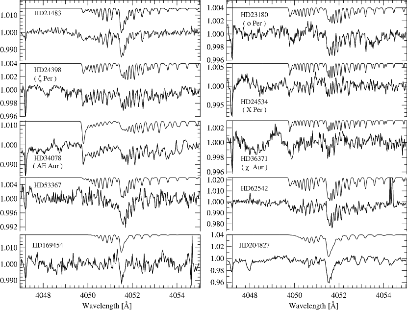
Figure 1.— Spectra of translucent sight lines toward which C₃ was detected, along with thermal excitation model fits. Note how the $Q$-branch at 4051.6 Å is very well fit, while the $R$ bandhead at 4049.8 Å is sometimes underestimated. Spectra are all shifted to rest wavelengths and the K i line at 4047.2 Å is marked by a vertical line. Broad stellar lines have been removed from the spectra of $\zeta$ Per, HD 21483, AE Aur, HD 36371, and HD 53367 using Gaussian line profiles.

Table 3Best Fit Parameters for Thermal Excitation Model of the Observed Spectra

Star	$N$(C3)	$N_{l}$(C3)	$N_{h}$(C3)	$T_{l}$	$T_{h}$	FWHM
						(km s-1)
HD 214830	4.60 $\pm$ 0.28	2.60	2.00	28.3 $\pm$ 1.3	150 $\pm$ 13	5.6 $\pm$ 0.1
HD 231800	1.27 $\pm$ 0.13	$\cdots$	$\cdots$	127.3 $\pm$ 3.9	$\cdots$	5.2 $\pm$ 0.2
HD 243980	1.30 $\pm$ 0.35	$\cdots$	$\cdots$	132 $\pm$ 10.3	$\cdots$	5.1 $\pm$ 0.4
HD 245340	1.77 $\pm$ 0.19	0.49	1.28	40 $\pm$ 6.1	250 $\pm$ 41	3.7 $\pm$ 1.0
HD 340780	6.21 $\pm$ 0.68	$\cdots$	$\cdots$	301.4 $\pm$ 15.4	$\cdots$	7.2 $\pm$ 0.3
HD 363710	0.75 $\pm$ 0.06	0.13	0.62	20.1 $\pm$ 2	250 $\pm$ 52	3.1 $\pm$ 1.2
HD 533670	2.08 $\pm$ 0.26	$\cdots$	$\cdots$	60.8 $\pm$ 1.5	$\cdots$	5.6 $\pm$ 0.1
HD 625420	10.37 $\pm$ 0.53	7.35	3.01	75.5 $\pm$ 7.2	200 $\pm$ 76	5.6 $\pm$ 0.1
HD 169454	2.24 $\pm$ 0.66	$\cdots$	$\cdots$	23.4 $\pm$ 1.4	$\cdots$	6.5 $\pm$ 0.4
HD 204827	11.13 $\pm$ 0.87	$\cdots$	$\cdots$	40.6 $\pm$ 0.8	$\cdots$	8.5 $\pm$ 0.2

3.1. Thermal Excitation Model

In this model the relative population of each rotational level ($J$$\leq$30) is determined using a thermal distribution at temperature, $T$. The fraction of total molecules in a particular $J$ level is given by

$$F_{J}(T)=\frac{2J+1}{q_{r}}exp\left(\frac{-hcB_{0}}{kT}J(J+1)\right)$$ (1)

where $q_{r}$ is the rotational partition function given by

$$q_{r}=\sum_{J\>even}^{\infty}(2J+1)e^{-hcB_{0}J(J+1)/kT}$$

For C₃ the ground state rotational constant $B_{0}$=0.43057 cm^-1 (Schmuttenmaer et al., 1990). The two parameters $T$ and $N$(C₃), along with the $f$-values shown in Table 2, then determine the equivalent width, $W_{J^{\prime},J^{\prime\prime}}$, of each transition using the standard relationship

$$W_{J^{\prime},J^{\prime\prime}}=8.853\times 10^{-21}\lambda^{2}N_{J}f_{J^{\prime},J^{\prime\prime}}\;\mathrm{\AA}$$ (2)

where $f_{J^{\prime},J^{\prime\prime}}$, the oscillator strength for a given transition $J^{\prime}\leftarrow J^{\prime\prime}$ at wavelength $\lambda$ in Å, is given by the product of the electronic oscillator strength $f_{ul}$, the Franck-Condon factor, and the Hönl-London factor. The units for $N_{J}$ and $W_{J}$ are cm^-2 and Å, respectively. Here we use $f$=0.016, consistent with Maier et al. (2001) and Oka et al. (2003), for the product $f$ of the electronic oscillator strength and Franck-Condon factor, whereas Roueff et al. (2002) and Galazutdinov et al. (2002) use $f$=0.0146. Future determinations of the oscillator strength and Franck-Condon factor will scale the derived column densities accordingly. The Hönl-London factors for this band ($\Lambda=1\leftarrow 0$) are $(J+2)/2(2J+1)$, 1/2, and $(J-1)/2(2J+1)$ for the $R$-, $Q$-, and $P$-branch transitions, respectively. Table 2 shows the adopted wavelengths, assignments and $f_{J^{\prime},J^{\prime\prime}}$ for each transition.

Beginning with an approximate estimate of the C₃ excitation temperature ($T$$\sim$45 K), column density ($N$(C₃)$\sim$10¹² cm^-2), and line width (FWHM=5.2 km s^-1) a simulated spectrum was produced. Standard curve-fitting routines were then used to minimize the difference between the observed and simulated spectra, by varying these three parameters ($T$, $N$(C₃), and FWHM). If a second temperature component was observed, in the form of a pronounced $R$-branch bandhead that was not reproduced with the single temperature simulation, then a spectrum incorporating two temperatures $T_{l}$ and $T_{h}$, and column densities $N_{l}$(C₃) and $N_{h}$(C₃) was used.

The initial estimate for the line width was larger than the instrument resolution ($\sim$4.5 km s^-1) and characteristic of the line widths in the observed spectra (Table 3). Broad lines are observed because translucent sight lines typically sample multiple diffuse clouds, which can have velocity separations comparable to, or larger than, our instrumental line width (Welty & Hobbs, 2001). The velocity distribution of the clouds, convolved with the instrumental line width, produces observed features that in some cases (e.g. HD 204827) are rather wide. Since we are observing through multiple clouds, the temperatures derived from our model represent an integrated average over all the clouds along the line of sight. In the opposite extreme, the best fit line widths for X Per and $\chi$ Aur are slightly below the instrument profile due to the relatively large level of noise in those spectra.

Figure 1 shows the observed spectra and best fit thermal excitation model for 10 detections, with model results summarized in Table 3. Measurement uncertainties are discussed in Section 3.3.

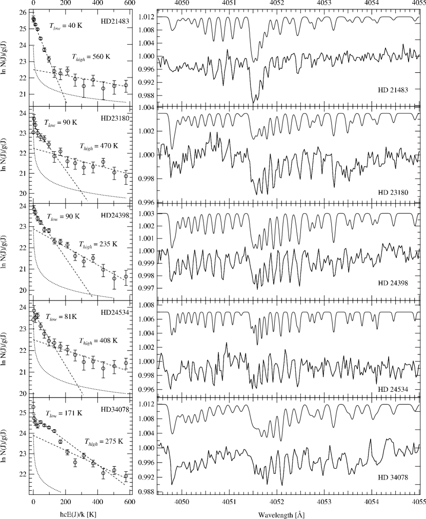
Figure 2.— Spectra of C₃ detections with rotational excitation model fit (offset for clarity) and the Boltzmann plot (left) derived from fit to individual rotational levels. The dotted curve depicts the 1$\sigma$ detection limit as a function of $J$. Points without error bars indicate upper limits. Dashed lines indicate fits to datapoints for $J$$\leq$14, and $J$$>$14, where the slope is inversely proportional to kinetic temperature. Note that the spectra are on different intensity scales and the very large columns of C₃ toward HD 62542 and HD 204827.

Fig. 2.— (continued)

3.2. Rotational Level Population Model

The most common method for determining the population of a particular rotational level $J$ is to measure the equivalent width $W$ of an unblended absorption feature. If multiple transitions ($\Delta J=0,\pm 1$) from the same lower $J$ state are observed, then each transition probes the same population and multiple measurements of the same quantity may be made.

In the case of our C₃ spectra, the low $J$ transitions ($J$$\lesssim$12) in the $R$-branch are well resolved, but the stronger $Q$-branch lines starting from the same $J$ levels pile atop one another. Similarly, transitions from higher $J$ levels that are well resolved in the $Q$-branch (e.g. $Q$(16) and $Q$(22)) are blended into a single feature in the $R$-branch bandhead. In order to extract information from all of the observed transitions, a model was used which varies the population in each $J$ level as a free parameter, produces a simulated spectrum, and then minimizes the difference between the observed and simulated spectrum.

The initial population values for the model were determined from the best fit thermal distribution. A curve fitting routine was then used to vary each $N_{J}$ and minimize the residuals. After fitting the population in each $J$ level, a Boltzmann plot was generated for each source, and kinetic temperatures which best fit $J$$\leq$14 and $J$$>$14 were determined. Figure 2 shows the observed and modeled spectra, with Boltzmann plots derived from the fit. The detection limits for each $J$ are shown as dotted lines in the Boltzmann plots. Results from the model are listed in Table 4 with uncertainties discussed below.

Table 4Rotational Level Populations Determined by Fitting the Observed Spectra

	$N_{J}$($\times 10^{11}$ cm-2)
$J$	HD 21483	HD 23180	HD 24398	HD 24534	HD 34078	HD 36371	HD 53367	HD 62542	HD 169454	HD 204827
0	1.22	0.09	0.34	0.14	0.88	0.15	0.94	2.64	0.49	1.83
2	5.79	0.92	1.01	1.04	2.55	0.27	2.83	6.46	2.13	15.42
4	7.67	1.21	1.54	1.35	3.65	0.42	3.04	10.04	4.66	22.54
6	8.34	1.18	1.69	2.14	4.51	0.42	3.93	12.96	4.73	24.27
8	6.19	1.26	1.84	1.72	7.06	0.21	3.17	15.15	2.27	19.44
10	3.87	1.43	1.61	1.49	7.53	0.29	2.34	11.59	$<$ 0.96	11.68
12	2.61	1.29	1.84	1.28	8.03	0.18	2.17	11.04	$<$ 0.96	6.53
14	1.43	0.82	1.30	1.36	7.85	$<$ 0.15	0.57	9.22	$<$ 0.96	4.24
16	1.42	1.19	1.44	1.31	5.30	0.17	0.67	6.94	$<$ 0.96	3.48
18	1.90	0.82	1.39	1.26	3.57	0.49	$<$ 0.31	5.54	$<$ 0.96	$<$ 0.76
20	1.26	0.82	0.91	1.10	2.38	0.32	0.51	4.36	$<$ 0.96	$<$ 0.76
22	0.90	0.73	0.78	0.87	3.65	0.26	$<$ 0.31	3.73	$<$ 0.96	$<$ 0.76
24	1.43	0.82	0.99	0.97	2.74	0.19	$<$ 0.31	2.74	$<$ 0.96	$<$ 0.76
26	0.91	1.13	0.62	0.76	1.83	$<$ 0.15	$<$ 0.31	1.19	$<$ 0.96	$<$ 0.76
28	1.14	0.72	0.44	0.91	2.28	$<$ 0.15	$<$ 0.31	0.73	$<$ 0.96	$<$ 0.76
30	1.28	0.64	0.52	1.12	1.83	0.44	0.42	0.64	$<$ 0.96	$<$ 1.15
$\delta N_{J}$	0.40	0.21	0.17	0.27	0.38	0.15	0.31	0.57	0.96	0.76

3.3. Uncertainties and Detection Limits

Uncertainties in the measurement of column densities for individual rotational levels are dependent on the uncertainty in the measurement of the equivalent width $W$. The 1$\sigma$ uncertainty in $W$ is given by

$$\delta W_{1\sigma}=(wd)^{1/2}\sigma$$ (3)

where $w$ is the FWHM of the observed transition (in Å), $d$ is the dispersion of the instrument (in Å pixel^-1), and $\sigma$ is the standard deviation of the normalized continuum–that is, (S/N)^-1. The $\delta W$ for each transition is converted to an uncertainty in population, $\delta N_{J}$ using Equation 2. For a given $J$ the transition with the largest oscillator strength will give the smallest uncertainty in $N_{J}$. In all cases except the $R(0)$ transition, the $Q$-branch has the largest oscillator strength for a given $J$ (see Table 2) and this is the $f$-value we use for our uncertainty estimate.

The detection limits for the total column of C₃ are dependent on the excitation of C₃. A larger total population of C₃ may go undetected if it is distributed among many rotational levels than if the population is all confined to a few low $J$ rotational levels. For our upper limits listed in Table 4.1 we assume that molecules are all distributed evenly among $J$=0 – 20. Although the choice of 11 levels among which the distribution is evenly spread is not based on any underlying physics, a comparison with the spectrum of $\zeta$ Per shows that for the purposes of estimating our detection limit, such an approach is not unreasonable.

3.4. The $R(0)$ Transition

During the initial analysis of the Boltzmann plots it became evident that $R(0)$ was uniformly underpopulated relative to what was expected from a thermal distribution that fit $J$=2 – 10. A close inspection of the spectra revealed that the observed $R(0)$ transition was significantly shifted toward the blue from the laboratory assignment of Gausset et al. (1965). This was particularly apparent in the spectrum of HD 62542, and can be noted by comparing the thermal excitation model (which uses the Gausset et al. (1965) assignment of $R(0)$) with our observations in Figure 1. Analysis of the higher resolution spectra of $\zeta$ Oph (Maier et al., 2001) and HD 152236 (Galazutdinov et al., 2002) shows similar indications of a spectral shift, however, neither dataset is of sufficient S/N to conclude that there is a significant difference between the observed spectrum and the laboratory assignment. Motivated by this discrepancy, a group including two of us (MÁ and BJM) revisited the laboratory spectrum of the 4051 Å band of C₃ with higher resolution than our observations (McCall et al., 2003a). Indeed, we found the $R(0)$ transition to be blue-shifted from the assignment of Gausset et al. (1965) and consistent with our astronomical spectra. Since $R(0)$ and $P(2)$ share the same upper state, our measurement of the $R(0)$ transition implies that the calculated position of the $P(2)$ line (Table 2) will shift to the blue and overlap $Q(8)$. This is confirmed by laboratory measurements (McCall et al., 2003a).

4. Results and Analysis

4.1. Column Density Comparisons

Table 5 Observed Properties of C₃ and C₂

Star	Name	$N$(C3)	$T_{low}$(C3)	$T_{high}$(C3)	$N$(C2)	$T$(C2)	$n_{coll}$(C2)	$N$(C2)/$N$(C3)
		($\times 10^{12}$ cm-2)	(K)	(K)	($\times 10^{14}$ cm-2)	(K)	(cm-3)
HD 21483		4.74 $\pm$ 0.28	40	560	1.10 $\pm$ 0.30	13 $\pm$ 5	190 $\pm$ 20	23.2 $\pm$ 6.5
		2.2 $\pm$ 0.5			0.93
HD 23180	$o$ Per	1.51$\pm$ 0.13	90	470	0.32 $\pm$ 0.12	60 $\pm$ 20	200 $\pm$ 50	21.2 $\pm$ 8.2
		$<$1.55			0.22 $\pm$ 0.03
HD 24398	$\zeta$ Per	1.83 $\pm$ 0.35	90	235	0.31 $\pm$ 0.08	80 $\pm$ 15	460 $\pm$ 150	17.0 $\pm$ 5.8
		1.0			0.19 $\pm$ 0.03
HD 24534	X Per	1.88 $\pm$ 0.19	81	408	0.76 $\pm$ 0.20	44 $\pm$ 5	225 $\pm$ 20	40.4 $\pm$ 11.6
		$\leq$1.5			0.53
HD 34078	AE Aur	6.56 $\pm$ 0.68	171	275	1.00 $\pm$ 0.09	120 $\pm$ 10	$>$500	15.2 $\pm$ 2.3
		2.2 $\pm$ 0.5			0.58
HD 36371	$\chi$ Aur	0.43 $\pm$ 0.06	38	554	0.29 $\pm$ 0.11	$\cdots$	$\cdots$	68.1 $\pm$ 27.9
		$<$1.29
HD 53367		2.21 $\pm$ 0.26	40	366	0.61 $\pm$ 0.16	$\cdots$	$\cdots$	27.6 $\pm$ 8.1
		$<$2.2
HD 62542		10.49 $\pm$ 0.53	75	137	0.8 $\pm$ 0.2	36 $\pm$ 15	510 $\pm$ 50	7.6 $\pm$ 1.9
HD 148184	$\chi$ Oph	2.50 $\pm$ 0.43			0.43 $\pm$ 0.05			17.2 $\pm$ 3.6
HD 149757	$\zeta$ Oph	1.6			0.25 $\pm$ 0.07			16.7 $\pm$ 5.5
		1.50 $\pm$ 0.29			0.24 $\pm$ 0.03
HD 152236		1.8 $\pm$ 0.29	66	$\cdots$	0.16 $\pm$ 0.06	36 $\pm$ 10	300 $\pm$ 100	13.3 $\pm$ 2.8
HD 169454		2.5 $\pm$ 0.66	42	$\cdots$	1.60 $\pm$ 0.29	50 $\pm$ 10	$>$500	64.0 $\pm$ 21.8
		4.3 $\pm$ 0.5			0.70 $\pm$ 0.14
HD 179406	20 Aql	2.0			0.82 $\pm$ 0.15
		1.3 $\pm$ 0.7			0.52
HD 204827		11.51 $\pm$ 0.87	43	$\cdots$	4.40 $\pm$ 0.29	49 $\pm$ 5	630 $\pm$ 200	38.3 $\pm$ 4.1
		10.4 $\pm$ 0.5
HD 210121		3.79			1.00 $\pm$ 0.13
		1.9 $\pm$ 0.5			0.65 $\pm$ 0.15

References. — (f) Oka et al. (2003); (g) Maier et al. (2001); (h) Roueff et al. (2002); (i) Galazutdinov et al. (2002); (j) van Dishoeck & Black (1986); (k) Federman et al. (1994); (l) Federman & Lambert (1988); (m) Gredel et al. (1992); (n) Gredel et al. (1993).

Note. — Non-detections of C₃ in this work (with the upper limit $N$(C₃) in 10¹¹ cm^-2 in parentheses) are: HD 11415 (1.8), HD 20041 (4.2), HD 21398 (3.3), HD 22951 (2.5), HD 24912 (1.6), HD 35149 (2.0), HD 37022 (2.1), HD 37061 (3.3), HD 41117 (1.8), HD 42087 (2.1), HD 43384 (2.6), HD 206267 (3.5), HD 207198 (6.1), HD 210839 (6.1). Oka et al. (2003) measure C₃ (with $N$(C₃) in 10¹² cm^-2 in parentheses) toward: HD 26571 (2.1$\pm$0.6), HD 27778 (1.2$\pm$0.3), HD 29647 (4.6$\pm$1.3), HD 172028 (3.6$\pm$0.6), HD 203938 ($\leq$1.3), HD 206267 (2.7$\pm$0.4).

Table 4.1 summarizes our measurements of $N$(C₃) along with previous work. In their determination of C₃ column densities from an extensive, low resolution survey, Oka et al. (2003) measured the equivalent width of the unresolved $Q$-branch and assumed that it contained half the total intensity of the C₃ band. While this is a good approximation for a thermal distribution at $T$$<$50 K, we note that this assumption underestimates the total column density when there is significant population in higher $J$ levels. Comparisons of $N$(C₃) for HD 204827 and HD 169454 show either agreement within error, or a slight overestimate by Oka et al. (2003). Notably, these are the two clouds for which we measure only a low temperature component in the excitation profile. On the other hand, AE Aur and HD 21483, which show pronounced $R$-branch bandheads (Figure 2), are underestimated by Oka et al. (2003) due to a significant population of C₃ in high rotational levels.

Our determination of $N$(C₃) for $\zeta$ Per is larger than the measurements of Maier et al. (2001) due to our higher S/N, which allows us to measure the populations in higher $J$ levels. The column density determination for $\zeta$ Oph by Roueff et al. (2002), using the data from Maier et al. (2001), is consistent with our measurements and highlights the utility of their model for determining $N$(C₃).

4.2. Correlations

The correlation between C₂ and C₃ pointed out by Oka et al. (2003) may be tested more rigorously with the precise determinations of the C₃ column density presented here. The $N$(C₂) measurements of Thorburn et al. (2003) are plotted against our measurements of $N$(C₃) in Figure 3.

The most notable outlier is HD 62542, which has an extremely high column density of C₃, yet an average to low column of C₂. The intriguing line of sight toward this star seems to be a highly unorthodox cloud; not only does it seem to be “missing” C₂, it has an extreme UV extinction curve (Cardelli & Savage, 1988), an unusually low column of CH⁺ (Cardelli et al., 1990), and it lacks the diffuse bands (DIBs) characteristic of reddened sightlines (Snow et al., 2002). Following the analysis of Cardelli et al. (1990), Snow et al. (2002) have interpreted the lack of DIBs toward this star by suggesting the sight line is dominated by a dense cloud stripped of its diffuse outer layers. Considering the weak DIBs and the seemingly low column of C₂, it is noteworthy that a correlation between C₂ and some DIBs, such as $\lambda$4963 and $\lambda$5769, has recently been identified (Thorburn et al., 2003). However, the “C₂ DIBs” are in general much weaker than the classical DIBs, such as $\lambda$6284 and $\lambda$5797, which have been reported to be unusually weak toward HD 62542 (Snow et al., 2002). Nonetheless, one might speculate that the processes which stripped the cloud of its strong DIBs may also have destroyed some of its C₂. On the other hand, it is unclear how C₃ would survive a process that destroys C₂, so one could suggest instead that the conditions in this cloud may favor carbon chain formation. Due to the peculiarity of the line of sight toward this star, we have excluded it from the correlation analysis.

Fitting all of our targets except HD 62542 shows a correlation between C₂ and C₃ similar to that observed by Oka et al. (2003). The correlation coefficient for this work is 0.898, whereas Oka et al. (2003) report 0.932. HD 169454 appears about 2$\sigma$ above the trendline in Figure 3, but the value of $N$(C₂) reported by Thorburn et al. (2003) is significantly larger than the values reported by van Dishoeck & Black (1989) and Gredel & Münch (1986), which are more consistent with the correlation measured here. AE Aur falls significantly below the trendline; perhaps the same processes that could have destroyed the DIBs and C₂ in HD 62542 have occurred, to a lesser extent, in AE Aur (Snow et al., 2002). Another consideration is the variability with time of the molecular species toward AE Aur, where $N$(CH) has increased by 20% over the last 10 years (Rollinde et al., 2003). However, there were only 2 years between the observations of C₂ and C₃ reported here, while either $N$(C₂) is a factor of $\sim$2 below or $N$(C₃) is a factor of $\sim$2 too large relative to the general trend observed for the other sight lines. The possible enhancement of $N$(C₃) is significantly larger than expected from the time variability of $N$(CH) alone.

Since HD 204827 has such a large column of C₃ relative to the rest of the sample, much of the correlation seems to rest on this datapoint. With the high sensitivity measurements of $N$(C₃) presented in this work, the correlation between C₂ and C₃ toward stars with relatively low column densities ($N$(C₃)$<$4$\times 10^{12}$cm^-2) may be tested. Excluding sources with $N$(C₃)$>$4$\times 10^{12}$cm^-2 (i.e. HD 204827, HD 62542, AE Aur, and HD 21483) and HD 169454 for reasons discussed above, we find a correlation coefficient of 0.841, supporting the correlation determined for the entire sample.

The observed correlation between C₂ and C₃ is strikingly similar to the correlation between C₂H and C₃H₂ measured by Lucas & Liszt (2000). In many cases the ratio of $N$(C₂)/$N$(C₃) listed in Table 4.1 falls within the mean abundance ratio $\left<\right.\mathrm{C}_{2}\mathrm{H}/o$-C${}_{3}\mathrm{H}_{2}\left.\right>$ = 27.7$\pm$8 measured by Lucas & Liszt (2000). It is unclear if this is coincidence or if there is some underlying chemistry which links these species and their relative abundances.

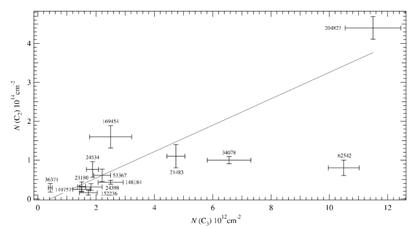
Figure 3.— Comparison of the column densities of C₃ and C₂. $N$(C₃) determined in this work is plotted against $N$(C₂) determinations of Thorburn et al. (2003) along with best fit (dotted) line. Error bars are 1$\sigma$.

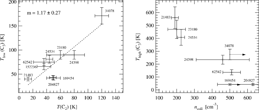
Figure 4.— Comparison of the excitation of C₃ and C₂. The excitation temperatures determined from the observed populations in low ($J$$\leq$14) levels of C₃ are compared to the kinetic temperatures determined from the observed excitation of C₂ and full excitation model of van Dishoeck & Black (1986) (left), showing good agreement. The excitation temperature determined from the high ($J$$>$14) levels of $C_{3}$ is compared to the densities derived from the C₂ excitation model (right). As expected, T_high(C₃) increases with decreasing density.

4.3. The Excitation of C₂

The excitation profile of C₃ was compared to the physical conditions determined by the well-understood rotational excitation of C₂. Table 4.3 summarizes previous observations in the literature of rotationally resolved C₂ toward the stars where we detected C₃. To the existing measurements we have added our C₂ spectrum of HD 204827 measured at Lick and the spectrum of X Per measured at Apache Point Observatory (Thorburn 2003, private communication).

Table 6 Observations of Interstellar C₂ Toward Various Stars

			$W_{\lambda}$ (mÅ)
$\lambda$ (Å)	Line	$f_{J^{\prime},J^{\prime\prime}}$	HD 21483	HD 23180	HD 24398	HD 24534	HD 34078	HD 62542	HD 149757	HD 152236	HD 169454	HD 204827
8757.69	R(0)	1.000	9.3 $\pm$ 1.2	1.3 $\pm$ 0.6	0.57 $\pm$ 0.17	1.2 $\pm$ 0.2	$\cdots$	4.4 $\pm$ 2	0.7 $\pm$ 0.3	0.7 $\pm$ 0.5	5.6 $\pm$ 1	12.8 $\pm$ 5.5
8753.95	R(2)	0.400	5.1 $\pm$ 1.6	1.4 $\pm$ 0.6	1.06 $\pm$ 0.17	1.9 $\pm$ 0.5	4.2 $\pm$ 1	9 $\pm$ 1	1.6 $\pm$ 0.3	1 $\pm$ 0.5	6 $\pm$ 0.5	18.3 $\pm$ 2.3
8761.19	Q(2)	0.500	11.5 $\pm$ 1.3	1.5 $\pm$ 0.6	1.19 $\pm$ 0.17	2.8 $\pm$ 0.2	3.2 $\pm$ 0.7	10 $\pm$ 1	1.2 $\pm$ 0.3	1.2 $\pm$ 0.5	6.6 $\pm$ 0.8	23.3 $\pm$ 1.8
8766.03	P(2)	0.100	5.6 $\pm$ 1.2	$\cdots$	$\cdots$	0.5 $\pm$ 0.2	$\cdots$	1 $\pm$ 0.5	$\cdots$	$\cdots$	1.3 $\pm$ 0.3	1.4 $\pm$ 3
8751.68	R(4)	0.333	$\cdots$	$\cdots$	0.82 $\pm$ 0.17	$\cdots$	3.4 $\pm$ 0.9	4.8 $\pm$ 1.2	$\cdots$	$\cdots$	$\cdots$	$\cdots$
8763.75	Q(4)	0.500	7 $\pm$ 1.3	1.7 $\pm$ 0.6	1.49 $\pm$ 0.17	2.9 $\pm$ 0.4	5.3 $\pm$ 0.6	7.1 $\pm$ 2	1.5 $\pm$ 0.3	0.9 $\pm$ 0.5	7.9 $\pm$ 0.7	15.7 $\pm$ 2.3
8773.43	P(4)	0.167	$\cdots$	$\cdots$	$\cdots$	$\cdots$	$\cdots$	2.6 $\pm$ 0.6	$\cdots$	$\cdots$	1.7 $\pm$ 0.8	$\cdots$
8750.85	R(6)	0.308	$\cdots$	1.7 $\pm$ 0.6	1.01 $\pm$ 0.17	3.2 $\pm$ 0.4	$\cdots$	2.8 $\pm$ 1	1.7 $\pm$ 0.3	$\cdots$	$\cdots$	7.2 $\pm$ 2.6
8767.76	Q(6)	0.500	8.1 $\pm$ 1.6	1.8 $\pm$ 0.6	$\cdots$	2 $\pm$ 0.1	4.6 $\pm$ 0.7	1.9 $\pm$ 0.9	1.4 $\pm$ 0.3	1 $\pm$ 0.5	3.9 $\pm$ 0.5	14.3 $\pm$ 1.1
8782.31	P(6)	0.192	$\cdots$	$\cdots$	$\cdots$	0.1 $\pm$ 0.3	$\cdots$	$\cdots$	$\cdots$	$\cdots$	$\cdots$	7.3 $\pm$ 1.7
8751.49	R(8)	0.294	$\cdots$	$\cdots$	0.37 $\pm$ 0.17	$\cdots$	$\cdots$	$\cdots$	$\cdots$	0.4 $\pm$ 0.4	$\cdots$	$\cdots$
8773.22	Q(8)	0.500	$\cdots$	0.8 $\pm$ 0.6	$\cdots$	$\cdots$	$\cdots$	3.2 $\pm$ 0.9	1.9 $\pm$ 0.3	$\cdots$	1.5 $\pm$ 0.5	$\cdots$
8792.65	P(8)	0.206	$\cdots$	$\cdots$	$\cdots$	3 $\pm$ 0.2	$\cdots$	$\cdots$	$\cdots$	$\cdots$	$\cdots$	$\cdots$
8753.58	R(10)	0.286	$\cdots$	$\cdots$	$\cdots$	0.7 $\pm$ 0.1	$\cdots$	$\cdots$	0.4 $\pm$ 0.3	$\cdots$	$\cdots$	$\cdots$
8780.14	Q(10)	0.500	$\cdots$	$\cdots$	$\cdots$	$\cdots$	$\cdots$	$\cdots$	$\cdots$	$\cdots$	1 $\pm$ 0.8	2.2 $\pm$ 0.8
	J		$N_{J}$ ($\times 10^{14}$)
	0		1.4 $\pm$ 0.2	0.19 $\pm$ 0.09	0.08 $\pm$ 0.03	0.17 $\pm$ 0.03	$\cdots$	0.6 $\pm$ 0.3	0.1 $\pm$ 0.04	0.1 $\pm$ 0.07	0.8 $\pm$ 0.2	1.89 $\pm$ 0.81
	2		3.1 $\pm$ 0.3	0.47 $\pm$ 0.14	0.37 $\pm$ 0.04	0.8 $\pm$ 0.06	1.1 $\pm$ 0.2	2.9 $\pm$ 0.2	0.45 $\pm$ 0.07	0.36 $\pm$ 0.11	2.1 $\pm$ 0.1	6.77 $\pm$ 0.4
	4		2.1 $\pm$ 0.4	0.5 $\pm$ 0.18	0.42 $\pm$ 0.04	0.86 $\pm$ 0.1	1.6 $\pm$ 0.2	2.2 $\pm$ 0.3	0.44 $\pm$ 0.09	0.26 $\pm$ 0.15	2.3 $\pm$ 0.2	4.61 $\pm$ 0.7
	6		2.4 $\pm$ 0.5	0.61 $\pm$ 0.15	0.48 $\pm$ 0.08	0.61 $\pm$ 0.04	1.4 $\pm$ 0.2	0.7 $\pm$ 0.2	0.52 $\pm$ 0.08	0.29 $\pm$ 0.15	1.2 $\pm$ 0.2	4.24 $\pm$ 0.3
	8		$\cdots$	0.24 $\pm$ 0.18	0.19 $\pm$ 0.09	2.14 $\pm$ 0.13	$\cdots$	0.9 $\pm$ 0.3	0.56 $\pm$ 0.09	0.1 $\pm$ 0.1	0.4 $\pm$ 0.2	$\cdots$
	10		$\cdots$	$\cdots$	$\cdots$	0.35 $\pm$ 0.08	$\cdots$	$\cdots$	0.21 $\pm$ 0.15	$\cdots$	0.3 $\pm$ 0.2	0.64 $\pm$ 0.2
	$n_{coll}$		190 $\pm$ 20	200 $\pm$ 50	460 $\pm$ 150	225 $\pm$ 20	$>$500	510 $\pm$ 50	115 $\pm$ 20	300 $\pm$ 100	$>$500	630 $\pm$ 200
	$T$		13 $\pm$ 5	60 $\pm$ 20	80 $\pm$ 15	44 $\pm$ 5	120 $\pm$ 10	36 $\pm$ 15	43 $\pm$ 20	36 $\pm$ 10	50 $\pm$ 10	49 $\pm$ 5

References. — (a) Federman et al. (1994); (b) Hobbs (1981); (c) Chaffee et al. (1980); (d) Private communication, Thorburn (2003); (e) Gredel et al. (1993); (f) Hobbs & Campbell (1982); (g) van Dishoeck & Black (1989); (h) This work.

All measured equivalent widths were converted to populations using the standard relationship in Equation 2. For multiple measurements of the same $J$ level, weighted averages were used for the population. The rotational populations were then simulated using the full C₂ excitation model of van Dishoeck & Black (1982), probing the density-temperature parameter space that determines the excitation of C₂ while minimizing the difference between the model and observed values. In this way a kinetic temperature $T$(C₂) and a derived density of collision partners, $n_{coll}$, was determined for all targets.

As detailed by van Dishoeck & Black (1982), the derived density $n_{coll}$ is dependent on the collision cross-section $\sigma_{0}$ of C₂ with H₂ or H and a scaling factor $I$ for the standard radiation field, which we assume to be 2$\times 10^{-16}$ cm² and 1, respectively. Changes in these values will scale $n_{coll}$ accordingly.

Figure 4 (left) shows a comparison of the temperature $T_{low}$(C₃) determined by fitting the low ($J$$\leq$14) rotational levels of C₃, with the kinetic temperature $T$(C₂) determined from the full excitation model of C₂. While not unexpected, there is an excellent relationship between the kinetic temperature and the low $J$ level population of C₃. One would expect the temperature measured by fitting the higher ($J$$>$14) rotational levels of C₃ to be inversely related to density, since as the density increases, collisional de-excitation is more efficient at reducing the high rotational level populations. This is indeed observed in the comparison of $T_{high}$(C₃) versus $n_{coll}$ and is shown in Figure 4 (right).

It is interesting to note that the C₃ columns measured toward HD 204827 and HD 169454, which are the two targets that have only low temperature components (Figure 2) due to their high densities ($n_{coll}$$>$500 cm^-3), are also the targets which deviate most from the trend in the relationship between $T_{low}$(C₃) and $T$(C₂). In these high density targets the kinetic temperature derived from C₂ and the temperature that best fits the excitation of C₃ are the same, whereas the low density ($n_{coll}$$<$500 cm^-3) sources all show a somewhat increased excitation temperature of C₃. This is because at high densities the excitation profiles of both C₂ and C₃ are predominantly determined by the kinetic temperature, whereas at low densities the low $J$ populations, along with the high-lying levels, have a contribution from radiative pumping.

5. Summary

We have observed rotationally resolved spectra of C₃ in 10 translucent sight lines. Using a new method of analysis to accurately retrieve the individual rotational level populations, comparisons have been made with the excitation of C₂, showing excellent agreement in the measurement of kinetic temperature. Trends with density are also consistent with the excitation expected for a non-polar linear molecule.

With these measurements we have shown that the correlation between $N$(C₂) and $N$(C₃), as pointed out by Oka et al. (2003), is maintained for sight lines with a range of $N$(C₃) from 4.3$\times 10^{11}$cm^-2 to 1.2$\times 10^{13}$cm^-2. The star HD 62542 does not fall on the correlation trendline between $N$(C₂) and $N$(C₃) and is shown to have either a very large column of C₃ or depletion in C₂, concomitant with the known weakness of diffuse band features in its spectrum. Similar processes may be occurring to a lesser extent in AE Aur.

Our measurements provide a new challenge for the full C₃ excitation model presented by Roueff et al. (2002), which has been heretofore limited by the quality of observational data.

References

- Black & Dalgarno (1977) Black, J. H., & Dalgarno, A. 1977, ApJS, 34, 405
- Cardelli et al. (1990) Cardelli, J. A., Edgar, R. J., Savage, B. D., & Suntzeff, N. B. 1990, ApJ, 362, 551
- Cardelli & Savage (1988) Cardelli, J. A., & Savage, B. D. 1988, ApJ, 325, 864
- Cernicharo et al. (2000) Cernicharo, J., Goicoechea, J. R., & Caux, E. 2000, ApJ, 534, L199
- Chaffee et al. (1980) Chaffee, F. H., Lutz, B. L., Black, J. H., van den Bout, P. A., & Snell, R. L. 1980, ApJ, 236, 474
- Clegg & Lambert (1982) Clegg, R. E. S., & Lambert, D. L. 1982, MNRAS, 201, 723
- Douglas (1951) Douglas, A. E. 1951, ApJ, 114, 466
- Douglas (1977) —. 1977, Nature, 269, 130
- Federman & Lambert (1988) Federman, S. R., & Lambert, D. L. 1988, ApJ, 328, 777
- Federman et al. (1994) Federman, S. R., Strom, C. J., Lambert, D. L., Cardelli, J. A., Smith, V. V., & Joseph, C. L. 1994, ApJ, 424, 772
- Galazutdinov et al. (2002) Galazutdinov, G., Pětlewski, A., Musaev, F., Moutou, C., Curto, G. L., & Krelowski, J. 2002, A&A, 395, 969
- Gausset et al. (1965) Gausset, L., Herzberg, G., Lagerqvist, A., & Rosen, B. 1965, ApJ, 142, 45
- Geballe et al. (1999) Geballe, T. R., McCall, B. J., Hinkle, K. H., & Oka, T. 1999, ApJ, 510, 251
- Gredel & Münch (1986) Gredel, R., & Münch, G. 1986, A&A, 154, 336
- Gredel et al. (1993) Gredel, R., van Dishoeck, E. F., & Black, J. H. 1993, A&A, 269, 477
- Gredel et al. (1992) Gredel, R., van Dishoeck, E. F., de Vries, C. P., & Black, J. H. 1992, A&A, 257, 245
- Haffner & Meyer (1995) Haffner, L. M., & Meyer, D. M. 1995, ApJ, 453, 450
- Herbig (1995) Herbig, G. H. 1995, ARA&A, 33, 19
- Hinkle et al. (1988) Hinkle, K. W., Keady, J. J., & Bernath, P. F. 1988, Science, 241, 1319
- Hobbs (1981) Hobbs, L. M. 1981, ApJ, 243, 485
- Hobbs & Campbell (1982) Hobbs, L. M., & Campbell, B. 1982, ApJ, 254, 108
- Hrivnak & Kwok (1999) Hrivnak, B. J., & Kwok, S. 1999, ApJ, 513, 869
- Huggins (1881) Huggins, W. 1881, R. Soc. Lond. Proc. Ser. I, 33, 1
- Jørgensen (1994) Jørgensen, U. G. 1994, in IAU Colloq. 146: Molecules in the Stellar Environment, ed. Jørgensen, U. G. pp.29-48, Springer-Verlag, Berlin
- Lucas & Liszt (2000) Lucas, R., & Liszt, H. S. 2000, A&A, 358, 1069
- Maier et al. (2001) Maier, J. P., Lakin, N. M., Walker, G. A. H., & Bohlender, D. A. 2001, ApJ, 553, 267
- McCall et al. (2003a) McCall, B. J., Casaes, R. N., Ádámkovics, M., & Saykally, R. J. 2003a, Chem. Phys. Lett., in press.
- McCall et al. (1998) McCall, B. J., Geballe, T. R., Hinkle, K. H., & Oka, T. 1998, Science, 279, 1910
- McCall et al. (2002a) McCall, B. J., Hinkle, K. H., Geballe, T. R., Moriarty-Schieven, G. H., Evans, N. J., II, Kawaguchi, K., Takano, S., Smith, V. V., & Oka, T. 2002a, ApJ, 567, 391
- McCall et al. (2003b) McCall, B. J., Huneycutt, A. J., Saykally, R. J., Geballe, T. R., Djuric, N., Dunn, G. H., Semaniak, J., Novotny, O., Al-Khalili, A., Ehlerding, A., Hellberg, F., Kalhori, S., Neau, A., Thomas, R., Osterdahl, F., & Larsson, M. 2003b, Nature, 422, 500
- McCall et al. (2002b) McCall, B. J., Oka, T., Thorburn, J., Hobbs, L. M., & York, D. G. 2002b, ApJ, 567, L145
- McCall et al. (2001) McCall, B. J., Thorburn, J., Hobbs, L. M., Oka, T., & York, D. G. 2001, ApJ, 559, L49
- Oka et al. (2003) Oka, T., Thorburn, J. A., McCall, B. J., Friedman, S. D., Hobbs, L. M., Sonnentrucker, P., Welty, D. E., & York, D. G. 2003, ApJ, 582, 823
- Raffety (1916) Raffety, C. W. 1916, Phil. Mag., 32, 546
- Rollinde et al. (2003) Rollinde, E., Boissé, P., Federman, S. R., & Pan, K. 2003, A&A, 401, 215
- Roueff et al. (2002) Roueff, E., Felenbok, P., Black, J. H., & Gry, C. 2002, A&A, 384, 629
- Rousselot et al. (2001) Rousselot, P., Arpigny, C., Rauer, H., Cochran, A. L., Gredel, R., Cochran, W. D., Manfroid, J., & Fitzsimmons, A. 2001, A&A, 368, 689
- Schmuttenmaer et al. (1990) Schmuttenmaer, C. A., Cohen, R. C., Pugliano, N., Heath, J. R., Cooksy, A. L., Busarow, K. L., & Saykally, R. J. 1990, Science, 249, 897
- Snow et al. (1988) Snow, T. P., Seab, C. G., & Joseph, C. L. 1988, ApJ, 335, 185
- Snow et al. (2002) Snow, T. P., Welty, D. E., Thorburn, J., Hobbs, L. M., McCall, B. J., Sonnentrucker, P., & York, D. G. 2002, ApJ, 573, 670
- Thorburn et al. (2003) Thorburn, J. A., Hobbs, L. M., McCall, B. J., Oka, T., Welty, D. E., Friedman, S. D., Snow, T. P., Sonnentrucker, P., & York, D. G. 2003, ApJ, 584, 339
- van Dishoeck & Black (1982) van Dishoeck, E. F., & Black, J. H. 1982, ApJ, 258, 533
- van Dishoeck & Black (1986) —. 1986, ApJS, 62, 109
- van Dishoeck & Black (1989) —. 1989, ApJ, 340, 273
- Vogt (1987) Vogt, S. S. 1987, PASP, 99, 1214
- Vogt et al. (1994) Vogt et al. 1994, Proc. Soc. Photo-Opt. Instr. Eng., 2198, p.362
- Welty & Hobbs (2001) Welty, D. E., & Hobbs, L. M. 2001, ApJS, 133, 345