On the Presence of Thermal SZ Induced Signal in the First Year WMAP Temperature Maps

Abstract

Using available optical and X-ray catalogues of clusters and superclusters of galaxies, we build templates of tSZ emission as they should be detected by the WMAP experiment. We compute the cross-correlation of our templates with WMAP temperature maps, and interpret our results separately for clusters and for superclusters of galaxies. For clusters of galaxies, we claim 2-5 $\sigma$ detections in our templates built from BCS (Ebeling et al., 1998, 2000), NORAS (Böhringer et al., 2000) and de Grandi et al. (1999) catalogues. In these templates, the typical cluster temperature decrements in WMAP maps are around 15-35 $\mu$K in the RJ range (no beam deconvolution applied). Several tests probing the possible influence of foregrounds in our analyses demonstrate that our results are robust against galactic contamination. On supercluster scales, we detect a diffuse component in the V & W WMAP bands which cannot be generated by superclusters in our catalogues (Einasto et al., 1994, 1997), and which is not present in the clean map of Tegmark, de Oliveira-Costa & Hamilton (2003). Using this clean map, our analyses yield, for Einasto’s supercluster catalogues, the following upper limit for the comptonization parameter associated to supercluster scales: $y_{SC}<2.18\times 10^{-8}$ at the 95% confidence limit.

1 Introduction

The WMAP experiment is currently observing the microwave sky at five different frequency channels with different angular resolution (Bennett et al., 2003a). The low frequency bands, K, Ka & Q, measuring at 23, 33 & 41GHz respectively, are expected to be particularly sensitive to the free-free and synchrotron emission in the Milky Way. Although their angular resolution is not as good as in the high frequency channels, their measurements of the foreground contamination are critical in order to achieve an optimal subtraction of non-cosmological signal in the overall analysis. This analysis has yielded the identification of two main components in the sky signal: a cosmological component, which constrains crucial cosmological parameters such as $\Omega_{\Lambda}$, $\Omega_{m}$, $n$, $\tau_{reion}$ with unprecedented accuracy (Bennett et al., 2003b), and a foreground-induced component, whose impact in the high frequency channels (V (61GHz) & W(94GHz)) is modelled by means of the low frequency measurements. These channels have been located in a frequency range where the contribution from foregrounds is expected to be minimal (Bennett et al., 2003c), and their high angular resolution (up to $0.21\degr$) enables the study the sub-horizon structure of the Last Scattering Surface.

However, it is also expected that the presence of Large Scale Structure intersecting the geodesics of the CMB photons leave a signature in the form of secondary temperature anisotropies. Among these temperature fluctuations, the most important (in terms of amplitude) are those caused by the Integrated Sachs-Wolfe effect, (ISW), due to the variation of the gravitational potential, and the thermal Sunyaev-Zel’dovich (hereafter tSZ, Sunyaev & Zeldovich (1980)), due to the distortion of the black body spectrum of CMB photons after interacting with a hot electron plasma. The search of tSZ-induced signal in CMB data sets by comparing them with surveys of Large Scale Structure has been performed for COBE data (Ganga, Cheng, Meyer, & Page, 1993; Boughn & Jahoda, 1993; Banday et al., 1996; Kneissl et al., 1997), and Tenerife data (Rubiño-Martín, Atrio-Barandela, & Hernández-Monteagudo, 2000). They all failed to measure any significant correlation, and hence could only set upper limits to the comptonization parameter $y$.

In this context, three recent analyses have been carried out on WMAP data. This first one has been carried out by the WMAP team: a cross-correlation of the W-band with the XBACs catalog of 242 Abell-type clusters (Ebeling et al., 1996) has prompted a detection at 2.5$\sigma$ level. However, a direct cross-correlation of WMAP data with ROSAT (Diego, Silk & Sliwa, 2003) has given negative results. In this analysis, the difference map between V and W bands was compared to the ROSAT map by the study of the power spectrum of the product map and the cross-power spectrum of both maps. Apart from an apparently spurious coincidence in the product map, there is no trace for any significant correlation. More recently, Boughn & Crittenden (2003) have reported a positive cross-correlation at the 2–3 sigma level between the WMAP data and the X-ray HEAO-1 and radio NRAO VLA sky surveys. Their study focuses on extra-galactic objects as tracers of the Large Scale Structure, and the positive sign of their correlation would point to the ISW effect as the responsible for this excess. A similar result was reported by Fosalba & Gaztañaga (2003) after cross-correlating the V band of WMAP with a template built from the APM galaxy survey. They find a positive cross correlation with a significance of $\sim 2\sigma$.

In this work, we extend the study of possible correlation of WMAP data with Large Scale Structure (LSS) to cluster and supercluster scales. By using cluster surveys present in the literature, we construct template maps of LSS, and cross correlate them with the temperature maps of WMAP. Although the angular resolution and the sensitivity of WMAP are not ideal for the typical tSZ amplitudes and angular profiles of clusters of galaxies, we expect that if a large enough number of them are indeed contributing to the map their final imprint should be statistically measurable. On the other hand, angular sizes of superclusters of galaxies are resolved by the V & W bands of WMAP, so they should allow to set constraints in the density and/or temperature of the diffuse gas thought to be present in those structures.

In Section 2 we outline the details of the statistical methods used in our analyses. Section 3 describes the WMAP data, whereas in Section 4 we explain how our tSZ templates of clusters and supercluster of galaxies were synthesised. Finally, in Section 5 we show our results, which we discuss in Section 6.

2 Statistical Method

In this section we describe the statistical tools used to search for signature of Large Scale Structure in WMAP CMB maps in the form of tSZ effect. All our statistics will be defined in the real space, and will be restricted to those regions where we expect a high contribution from SZ sources. By doing this, we are trying to minimise the effects related to the limited angular resolution and sensitivity of WMAP in terms of typical SZ amplitudes. A Fourier analysis in a selected and non-continuous sample of pixels cannot always be defined in a simple way and will be discarded here. Core radii of clusters of galaxies usually subtend an angle of $\simeq 1^{\prime}-3^{\prime}$ in the sky, which is considerably smaller than the FWHM of the highest resolution channel (94GHz) of WMAP, ($\sim 12.6$ arcmins). For this reason, from the five bands of WMAP, we shall only use this channel when searching for cluster induced signal in the WMAP data, as we expect that other channels will dilute the SZ signal to a much greater extent. The high resolution map of Tegmark, de Oliveira-Costa & Hamilton (2003), which combines all bands but preserves the angular resolution of the 94GHz channel, will also be considered. However, for superclusters of galaxies, the situation differs considerably, provided the fact that these sources can have a size of a few degrees on the sky, enabling the use of lower frequency channels of WMAP.

The two statistical methods used in this paper will search for similarities present in both our templates and the WMAP CMB maps. The first method (method i) consists of a pixel-to-pixel comparison of CMB maps to the templates. Given the CMB and noise amplitudes in those pixels, we estimate what is the fraction of signal present in CMB maps which is correlated to the structure of our catalogues. In the second method, (method ii) we computed the cross-correlation function between our templates and the WMAP map(s), and compared it to the auto-correlation function computed in our synthesised maps.

We shall assume that the WMAP data can be modelled as the following sum of components:

$$\mbox{\bf{T}}=\mbox{\bf{T}}_{cmb}+\alpha\mbox{\bf{M}}+\sum_{i}c_{i}\mbox{\bf{F}}^{i}+\mbox{\bf{N}},$$ (1)

where $\mbox{\bf{T}}_{cmb}$ denotes the CMB, N the noise, and M is the SZ induced signal modelled by our templates, which enters into the map with an average amplitude given by $\alpha$. $c_{i}\mbox{\bf{F}}^{i}$ denotes the ith foreground component. This last term will introduce a bias in our statistics, and its impact in our results must be considered. There might be as well some offset due to the inaccurate setting of the zero level in the WMAP maps. From figure (7) in Bennett et al. (2003c) one would expect a typical error of a few ($\sim 3-5$) microkelvin. The impact of such offsets will be addressed when quoting our results.

Method i):
We shall minimise the statistic $\chi^{2}$ given by

$$\chi^{2}=(\mbox{\bf{T}}-\alpha\mbox{\bf{M}}){\cal C}^{-1}(\mbox{\bf{T}}-\alpha\mbox{\bf{M}})^{T}$$ (2)

in terms of $\alpha$. By doing this, our estimate of $\alpha$ will be equal to:

$$E[\alpha]=\frac{\mbox{\bf{T}}{\cal C}^{-1}\mbox{\bf{M}}^{T}}{\mbox{\bf{M}}{\cal C}^{-1}\mbox{\bf{M}}^{T}}$$ (3)

In both equations 2 and 3, ${\cal C}$ denotes the correlation function of the SZ-free temperature map, i.e.:

$${\cal C}=<(\mbox{\bf{T}}-\alpha\mbox{\bf{M}})^{T}(\mbox{\bf{T}}-\alpha\mbox{\bf{M}})>$$ (4)

In our analyses, we considered only CMB and noise when computing ${\cal C}$. The cosmological signal was modelled by using the CMB power spectrum measured by the WMAP team (Bennett et al., 2003a), whereas the noise component was introduced using the amplitudes at each pixel according to the scanning strategy of the WMAP mission. The formal error for the estimated $\alpha$ is given by:

$$\sigma_{\alpha}=\sqrt{\frac{1}{\mbox{\bf{M}}{\cal C}^{-1}\mbox{\bf{M}}^{T}}}$$ (5)

However, in these equations we have neglected the bias term introduced by the presence of any possible foreground component, (i.e. synchrotron, free-free, dust or point sources). Our basic assumption will be that foregrounds and tSZ sources will introduce temperature fluctuations of opposite sign, positive and negative respectively, in the WMAP CMB scans. We remark at this point that all WMAP channels are in the Rayleigh-Jeans (RJ) frequency range, for which the tSZ distortions of the CMB planckian spectrum introduce negative temperature fluctuations. Therefore, because of the presence of foreground residuals in WMAP maps, the measured $\alpha$ will be shifted to positive values, and we will only be able to establish lower limits to the presence of SZ-induced signal in WMAP scans, so our approach can be regarded as conservative.

Method ii):
We shall define the $\chi^{2}$ statistic in terms of the cross-correlation and auto-correlation functions computed from the WMAP CMB map(s) and our templates. In this case, we write $\chi^{2}$ in the form:

$$\chi^{2}=\sum_{ij}\left[C_{TM}(\theta_{i})-\alpha C_{MM}(\theta_{i})\right]$$

$$\phantom{xxxxxxxxxxxxxxxxxxx}{\mbox{\bf$\pi$}}^{-1}_{ij}\left[C_{TM}(\theta_{j})-\alpha C_{MM}(\theta_{j})\right]$$ (6)

In this equation, $C_{TM}$ and $C_{MM}$ denote the cross and auto correlation function of our template maps with the WMAP scans, respectively. $\pi$ is the covariance matrix, defined as:

$${\mbox{\bf$\pi$}}_{ij}=$$

$$\langle\;\left(C_{TM}(\theta_{i})-\langle C_{TM}(\theta_{i})\;\rangle\;\right)\;\left(C_{TM}(\theta_{j})-\langle C_{TM}(\theta_{j})\;\rangle\;\right)\;\rangle.$$ (7)

The angle brackets denote ensemble averages after computing the cross-correlation between our templates and 100 Monte-Carlo realizations of the microwave sky accounting for the CMB signal and instrumental noise. The value of $\alpha$ which minimises $\chi^{2}$ and its formal error are given by the following equations:

$$E[\alpha]=\frac{\sum_{ij}C_{TM}(\theta_{i}){\mbox{\bf$\pi$}}^{-1}_{ij}C_{MM}(\theta_{j})}{\sum_{ij}C_{MM}(\theta_{i}){\mbox{\bf$\pi$}}^{-1}_{ij}C_{MM}(\theta_{j})}$$ (8)

$$\sigma_{\alpha}=\left[\sum_{ij}C_{MM}(\theta_{i}){\mbox{\bf$\pi$}}^{-1}_{ij}C_{MM}(\theta_{j})\right]^{-\frac{1}{2}}$$ (9)

This method assumes that all components which are not correlated to the template M average to zero when computing the cross-correlation. Foregrounds do not average to zero, and so they are supposed to bias the estimation of $\alpha$ towards positive values. Therefore, the impact of foregrounds in this analysis is quite similar to that in the previous method. We must also note that any mismatch in the zero level of the map would yield spurious correlation, so it is convenient to make alternative tests, such as repeating analyses after rotating the templates, to check whether any measured cross correlation is actually associated to our templates or not.

We expect method ii to be particularly sensitive to the spatial structure of superclusters of galaxies. Indeed, under WMAP’s 94 GHz beam, almost all clusters can be regarded as point-like, so we should expect $C_{MM}(\theta)=0$ for $\theta>\theta_{FWHM}$. However, superclusters of galaxies can subtend up to 40 degrees in the sky, and for them it might be possible to trace their typical angular extent by the study of $C_{TM}(\theta)$. For these reasons, we shall use method i for the search of tSZ signal in cluster scales, whereas method ii will be applied on supercluster templates. Due to the typical size of superclusters (few degrees), one can include in the analysis different bands of WMAP, as we show in the following section. Nevertheless, it is worth to remark that, in terms of the frequency dependence of the tSZ effect, the signal should drop around a 14% from channel V to channel W.

3 The WMAP data

We have mentioned that, due to angular resolution requirements, initially we considered only the W band for our analyses with templates of clusters of galaxies. Nevertheless, for the sake of comparison, we included the map provided by Tegmark, de Oliveira-Costa & Hamilton (2003), here denoted as T03. This map weights the five bands of WMAP according to their sensitivity at every angular scale. The result is a map with as much angular resolution as the W band and smaller presence of both noise and foreground contaminants. However, the properties of its noise component are complex. In our analyses, we characterised it in a optimistic and/or in a conservative way: either we assumed that the excess power of the map ($\sigma_{excess}\simeq 66\mu$K) was due to gaussian white noise, or we simply assigned WMAP’s 94GHz band noise pattern to T03.

In order to assess the impact of foregrounds on our results, we performed our analyses using two different foreground masks: the Kp0 mask and the Kp2 mask, both provided by the WMAP team. These masks remove from the analysis those pixels showing temperature fluctuations that trespass a given threshold computed from the histogram of the K-band data. The digit in the name of the mask is proportional to the threshold, so Kp0 is twice as conservative/strict as Kp2. In these analyses, the HEALPix resolution parameter was $N_{side}=$512.

The relatively large typical size of superclusters allowed us to test the consistency of our results by including the V band in our analyses. Furthermore, clean maps (in the sense of foreground-free) provided by the WMAP team (here denoted as ilc for internal linear combination map) and by Tegmark, de Oliveira-Costa & Hamilton (2003) were also considered. The ilc map has a typical angular resolution of one degree, whereas T03 has as much angular resolution as the W map. However, at low angular resolution, both maps are very similar, so we only retained T03 in our analyses. For our purposes of studying superclusters, the resolution of one degree suffices, so those temperature maps and all supercluster templates where pixelized under a coarser resolution, of a pixel size of $\sim 56^{\prime}$. This angular degradation allowed us to speed the computation of the cross-correlation between the WMAP temperature maps and our supercluster templates, and also made feasible to estimate the covariance matrices of equation (7) under a reasonable amount of time. We expect that the linear combination of different bands used to build the T03 map does not remove the tSZ component of our maps, but leaves it in roughly the same amplitude level. Our results will justify this hypothesis.

4 Templates

One crucial step in our procedure will be constructing the templates from existing surveys of clusters and superclusters of galaxies, both in the optical and in the X-range band. We shall build only tSZ templates, that is, in units of decrements of thermodynamic temperature. When cross-correlating with WMAP temperature maps, a positive correlation would point to a detection of tSZ effect. In any case, what matters is the spatial structure of our templates and not their overall normalisation. The conversion into thermodynamic temperature decrements from X-ray based catalogues will be performed by using existing relations between flux and/or luminosity in the X-ray band and antenna temperature decrements. For the optical catalogues, further assumptions will be necessary.

In the case of galaxy clusters, there is a fairly large sample of catalogues available, both in the X-range and in the optical. In the northern sky, our analyses will first focus on two X-ray based catalogues of clusters of galaxies, i.e., the Northern ROSAT All Sky Galaxy (NORAS) Cluster Survey (Böhringer et al., 2000) and the ROSAT Brightest Cluster Sample (BCS, Ebeling et al. (1998, 2000)). The source of these two catalogues is the published data of the ROSAT All Sky Survey (RASS, Trümper (1993), Vogues et al. (1999)). The NORAS cluster survey contains 495 sources with extended X-ray emission, of which 378 are unambiguously identified as clusters of galaxies. Due to the modest completeness of this catalogue, (count-rate limit of 0.06 counts/s), we extend our analysis to the BCS catalogue, which is flux limited and shows a completeness of around 90%. This catalogue is built on two different cluster samples: the first sample (Ebeling et al., 1998) listed 201 clusters of galaxies, whereas the extended sample (Ebeling et al., 2000) provided 99 new objects. The criteria used in their construction are not purely X-ray based. Both catalogues (NORAS and BCS) give luminosities in the 0.1–2.4 keV energy band for every cluster, which will be converted into brightness temperature fluctuations, as it will be shown.

In the southern hemisphere, de Grandi et al. (1999) extracted from the RASS data a flux limited sample of 130 clusters of galaxies, with an estimated completeness of around 90 %. Redshifts and fluxes in the 0.5 – 2 keV energy band are given for every object.

Analysing ROSAT Position Sensitive Proportional Counter pointings, Vikhlinin et al. (1998) compiled a catalogue of 203 serendipitously detected galaxy clusters. This catalogue, hereafter denoted by V98, covers both hemispheres, and therefore complements all catalogues listed above. V98 provides redshifts and fluxes of members in the energy range of 0.5 – 2 keV. A conversion into luminosities will be necessary in order to estimate the antenna temperature fluctuations induced by these clusters. All catalogues listed so far rely on ROSAT data, and hence are all conditioned by the observation strategy of this experiment.

For the sake of comparison, we shall include in the analysis two more catalogues of galaxy clusters. These remaining two catalogues were built on the basis of existing optical galaxy cluster surveys, namely APM (Dalton et al., 1997) and ACO (Abell, Corwin & Olowin, 1989). These catalogues provide an homogeneous sample of galaxy clusters in both hemispheres, and have been processed after applying selection criteria well different from those used in X-ray data analysis. However, unlike in the previous cases, these catalogues are not directly sensitive to the hot gas causing SZ distortions, and assumptions will have to be made when relating optical properties of the sources (i.e. richness) with antenna temperature decrements. Given the angular resolution of the W band, we note that we can safely ignore issues related to the gas distribution within cluster scales.

With respect to superclusters, we shall recur to the catalogues provided by Einasto et al. (1994, 1997). The use of these templates will be essential when testing the hypothesis of the presence of diffuse hot gas distributed in megaparsec scales.

Table 1: SZ cluster sample used to calibrate the template maps

Cluster Name	z	$\Delta T_{SZ}^{RJ}\;{}^{(a)}$	$L_{X}^{(0.1-2.4keV)}\;{}^{(b)}$
		(mK)	($10^{44}~{}h_{50}^{-2}~{}erg~{}s^{-1}$)
A1656(COMA)	0.0232	$-0.55\pm 0.10$	7.26
A2256	0.0601	$-0.44\pm 0.09$	7.11
A2142	0.0899	$-0.90\pm 0.14$	20.74
A478	0.09	$-0.92\pm 0.15$	13.19
A1413	0.143	$-0.96\pm 0.11$	13.28
A2204	0.152	$-0.96\pm 0.28$	21.25
A2218	0.171	$-0.75\pm 0.20$	9.30
A665	0.182	$-0.91\pm 0.09$	16.33
A773	0.197	$-0.89\pm 0.10$	13.08
A1835	0.252	$-1.34\pm 0.15$	38.53
Z3146	0.291	$-0.86\pm 0.14$	26.47

(a) Central decrement, from the compilation of Cooray (1999).
(b) X ray luminosities from the BCS catalogue.

The last step in our template construction procedure was assigning temperature decrements to the sources in our catalogues. For the case of galaxy clusters in X-ray based catalogues, it was done in the same way than Cooray (1999), by relating $\Delta T_{tSZ}$ with $L_{X}$ from a sample of clusters with measured RJ antenna temperature decrements Following his discussion, we would expect this relation to have the form $\Delta T_{tSZ}=aL_{x}^{b}$. A $\chi^{2}$ minimisation was used to derive the best-fit pair $(a,b)$, using luminosities in the 0.1-2.4 keV ROSAT band from the BCS catalogue

$$\Delta T_{tSZ}^{RJ}=-(0.24\pm 0.06)\Bigg{(}\frac{L_{X}^{(0.1-2.4keV)}}{10^{44}~{}h_{50}^{-2}~{}erg~{}s^{-1}}\Bigg{)}^{0.47\pm 0.09}\;mK$$ (10)

The values used for this fit are summarised in table (1). A similar fit can be obtained from the luminosities quoted in the NORAS catalogue ($a=0.21\pm 0.05$, $b=0.53\pm 0.09$). Clusters extracted from the RASS-PSC catalogue had fluxes in the same energy range than NORAS and BCS (0.1 – 2.4 keV), so a conversion into flux and $\Delta T_{tSZ}$ was straightforward. For V98 and the southern catalogue of de Grandi et al. (1999), a previous scaling of fluxes from the 0.5 – 2 keV energy band into the 0.1 – 2.4 keV band was first required (we obtained an average conversion factor of $F_{x}(0.5-2keV)/F_{x}(0.1-2.4keV)\approx 0.65$). For optically selected clusters (ACO and APM catalogues), we have assumed that the observed SZ decrement is proportional to some power $n$ of the cluster richness $R$. Following (Bennett et al., 1993), we have probed here their values $n=1,2,3$. In addition, we have used the cluster sample described in table (1) to calibrate a relation with the form $L_{X}=A(R+1)^{n^{\prime}}$, obtaining

$$L_{X}^{(0.1-2.4keV)}=(1.6\pm 0.3)(R+1)^{1.4\pm 0.2}\;10^{44}~{}h_{50}^{-2}~{}erg~{}s^{-1}$$ (11)

We finally related $L_{X}$ with $\Delta T_{tSZ}$ by using the scalings given above. This template will be labelled as ACO calibrated.

We conducted two different approaches when modelling the templates of superclusters of galaxies. We first introduced an uniform distribution of hot gas centred on the optical center of the supercluster and with radius the angular size of the supercluster, as it is provided by the catalogues. This template will be referred to as Sph-SC for Spherical Superclusters, and will probe the presence of hot gas in SC scales. However, some correlation present between these structures and the WMAP CMB maps might be diluted due to the huge angular size ($\theta_{SC}\sim 40\degr$) of some members. For this reason, our second approach consisted in filling with hot gas a circle of radius one degree around every cluster member in each supercluster. In some occasions, these circles overlap along a given direction in those superclusters where member clusters align forming a filamentary structure. We shall label this template as r1dg-SC. We assumed that the spheres of hot gas in both Sph-SC and r1dg-SC templates had the same density and temperature in every case, and so we assigned identical tSZ decrements to all of them.

There were two types of sources in our templates, according to their angular size. Point-like sources refer to all those clusters which are not resolved by the W channel of WMAP . Extended sources refer to COMA, VIRGO and superclusters. In all cases, the templates have been convolved with a realistic approximation of the average WMAP 94GHz beam. In this initial stage, the pixelization of all templates was such that the typical pixel size was around $7^{\prime}$, ($N_{side}=512$ under HEALPix pixelization). In the case of superclusters, the templates were degraded down to $N_{side}=64$, which corresponds to a pixel size of $\sim 54^{\prime}$. Therefore, for superclusters, templates do not contain $3,145,728$ pixels, but just $49,152$ pixels.

5 Results

5.1 Cluster templates

In the present section we search for correlations between our cluster templates and WMAP CMB scans. After building the cluster templates, they were convolved with the symmetrised window functions corresponding to each of the four differencing assemblies (hereafter DA’s) present in the W-band. These convolved templates were weighted according to the noise pattern of each DA, yielding a final template which was produced in exactly the same way as the averaged CMB map corresponding to the W-band of WMAP. In order to investigate which clusters contributed to the CMB maps, we applied three different amplitude masks, so only pixels brighter than some threshold would be used when searching for correlation. In practice, it consisted in computing the histograms of pixel amplitudes for each template. These histograms typically showed a symmetric distribution around zero amplitude (due to the numerical noise introduced by the convolution) plus a bright tail, formed by cluster pixels. By increasing/lowering the threshold amplitude we merely change the number of pixels in the tail considered in the analyses. For the three masks of increasing amplitude, hereafter labelled as $\nu_{1}$, $\nu_{2}$ & $\nu_{3}$, we selected a sample of 2000, 500 and 50 pixels, respectively.

We used four different CMB maps in this section. One of them was the W band of WMAP. This channel contains a white noise of an average amplitude of 175$\mu$K, which makes it significantly more noisy than the map provided by Tegmark, de Oliveira-Costa & Hamilton (2003). For comparison, we included this map (T03) in our analyses as well. Furthermore, in order to check for systematic effects in our approach, we repeated the analyses after rotating both maps 5 degrees around the axis orthogonal to the Galactic plane, i.e., $\delta l=5\degr$. The rotated maps will be labelled as R-W and R-T03 for W and T03, respectively. By comparing results from W and T03 to R-W and R-T03, we can i) check how our error bars compare with the case of lack of correlation, and ii), check that any detected correlation vanishes in the rotated map, so that we can assign such correlation to sources of angular size $<5\degr$. As mentioned earlier, we try to track the impact of foregrounds by performing our analyses in both Kp0 and Kp2 masks.

All results are shown in table (2), for the Kp0 mask. In this table we define $\beta$ as $\beta\equiv\alpha\langle\mbox{\bf{M}}\rangle$, where M denotes the template. That is, $\beta$ is given in temperature units ($\mu K$), and contains the sign of the cross-correlation, i.e., negative for tSZ. From this table, one can deduce that three catalogues are giving some significant tSZ induced signal, namely BCS, NORAS and de Grandi. For all of them, the statistical significance of the detection is higher under the column T03. This is partially associated to the fact that in this case, we are taking the optimistic values of the noise level for the T03 map. The pessimistic approach would consist in quoting the values of $\beta$ under the T03 column but with the error bars given in the W column. We must remark, however, that the error bars quoted in the optimistic case are not far from (but rather well within) the null (i.e., free of tSZ emission) values of $\beta$ quoted under the R-T03 column. With respect to optical catalogues, we can appreciate that the APM catalogue at $n=2,3$ in T03 gives values for $\beta$ which are consistently increasing with increasing $\nu$, surpassing the threshold of 2$\sigma$ in $n=3$, $\nu_{1}$. This trend might be clarified with the second year WMAP data release, for which noise amplitude is expected to be a factor of $\sqrt{2}$ lower. In all cases where we claim detection, $\Delta T_{tSZ}$ increases with the threshold, although its statistical significance diminishes as a consequence of the smaller amount of pixels. The only slight increase of tSZ amplitude with the threshold assures that the correlation is raised not exclusively by the very brightest clusters, but by most of the clusters considered in each catalogue. Otherwise, the signal would be much more diluted with decreasing $\nu$. Note that these amplitudes give the average contribution of the tSZ effect to WMAP maps, and have to be corrected for the beam and pixel smearing in order to give the actual cluster decrements. These analyses were repeated with zero-mean CMB maps, yielding similar results. The presence of possible offsets in the CMB maps therefore has negligible impact on our conclusions.

xxxxxxxxxxxxxxxxx $\beta\pm\sigma_{\beta}$, ($\mu$K), [Kp0]
Template Catalogue		W	R-W	T03	R-T03
	$\nu_{1}$	20.34 $\pm$ 6.83	18.57 $\pm$ 6.84	-1.32 $\pm$ 4.75	5.21 $\pm$ 4.82
ACO ($L_{X}=L_{X}(R+1)$)	$\nu_{2}$	17.21 $\pm$ 11.26	13.23 $\pm$ 11.32	-2.40 $\pm$ 7.60	2.72 $\pm$ 7.64
	$\nu_{3}$	32.35 $\pm$ 28.69	12.46 $\pm$ 28.54	24.36 $\pm$ 18.10	-1.49 $\pm$ 18.27
	$\nu_{1}$	13.44 $\pm$ 6.65	13.89 $\pm$ 6.64	0.54 $\pm$ 3.78	-0.35 $\pm$ 3.84
ACO (n=1)	$\nu_{2}$	16.22 $\pm$ 10.80	11.31 $\pm$ 10.85	-3.41 $\pm$ 7.03	-0.08 $\pm$ 7.14
	$\nu_{3}$	20.69 $\pm$ 28.13	-23.49 $\pm$ 27.96	5.36 $\pm$ 17.29	-35.93 $\pm$ 17.56
	$\nu_{1}$	6.93 $\pm$ 6.02	9.83 $\pm$ 6.05	-0.54 $\pm$ 3.13	-2.72 $\pm$ 3.22
ACO (n=2)	$\nu_{2}$	2.76 $\pm$ 10.91	4.72 $\pm$ 11.07	-6.81 $\pm$ 6.27	-3.99 $\pm$ 6.54
	$\nu_{3}$	16.47 $\pm$ 28.41	-29.00 $\pm$ 28.50	5.19 $\pm$ 17.36	-30.98 $\pm$ 18.00
	$\nu_{1}$	-0.07 $\pm$ 4.79	4.36 $\pm$ 4.91	-2.40 $\pm$ 2.26	-2.26 $\pm$ 2.41
ACO (n=3)	$\nu_{2}$	0.66 $\pm$ 10.23	2.34 $\pm$ 10.44	-3.81 $\pm$ 5.53	-3.33 $\pm$ 5.91
	$\nu_{3}$	-24.07 $\pm$ 30.24	-34.18 $\pm$ 30.92	-22.77 $\pm$ 17.74	-10.30 $\pm$ 19.30
	$\nu_{1}$	-3.37 $\pm$ 8.94	-2.22 $\pm$ 8.93	-5.67 $\pm$ 4.16	-3.89 $\pm$ 4.15
APM (n=1)	$\nu_{2}$	-2.19 $\pm$ 15.96	6.15 $\pm$ 15.95	-7.57 $\pm$ 10.40	-11.41 $\pm$ 10.42
	$\nu_{3}$	3.77 $\pm$ 31.99	29.28 $\pm$ 32.05	-3.05 $\pm$ 21.92	2.82 $\pm$ 22.09
	$\nu_{1}$	-5.58 $\pm$ 5.74	1.57 $\pm$ 5.76	-3.24 $\pm$ 2.55	-3.69 $\pm$ 2.58
APM (n=2)	$\nu_{2}$	-10.63 $\pm$ 12.45	9.96 $\pm$ 12.45	-9.62 $\pm$ 6.27	-9.10 $\pm$ 6.30
	$\nu_{3}$	-0.54 $\pm$ 31.73	36.01 $\pm$ 31.78	-13.10 $\pm$ 19.49	-3.33 $\pm$ 19.95
	$\nu_{1}$	-4.16 $\pm$ 3.39	-0.01 $\pm$ 3.43	-3.52 $\pm$ 1.48	-1.50 $\pm$ 1.52
APM (n=3)	$\nu_{2}$	-6.62 $\pm$ 9.07	5.25 $\pm$ 9.17	-5.93 $\pm$ 4.10	-7.19 $\pm$ 4.22
	$\nu_{3}$	-20.71 $\pm$ 30.95	30.18 $\pm$ 31.09	-17.91 $\pm$ 18.20	-8.31 $\pm$ 18.84
	$\nu_{1}$	-3.75 $\pm$ 3.05	-0.32 $\pm$ 2.98	-7.24 $\pm$ 1.32	-0.14 $\pm$ 1.29
de Grandi	$\nu_{2}$	2.10 $\pm$ 10.45	2.75 $\pm$ 10.27	-21.49 $\pm$ 5.19	5.31 $\pm$ 5.01
	$\nu_{3}$	6.37 $\pm$ 28.68	-27.48 $\pm$ 28.47	-48.58 $\pm$ 17.72	25.55 $\pm$ 17.41
	$\nu_{1}$	-18.10 $\pm$ 5.30	6.61 $\pm$ 5.37	-8.44 $\pm$ 2.50	-2.76 $\pm$ 2.57
BCS	$\nu_{2}$	-29.87 $\pm$ 11.40	16.66 $\pm$ 11.62	-19.00 $\pm$ 6.63	-8.25 $\pm$ 6.81
	$\nu_{3}$	-64.06 $\pm$ 31.78	19.59 $\pm$ 31.96	-39.30 $\pm$ 18.43	-12.30 $\pm$ 18.62
	$\nu_{1}$	-10.95 $\pm$ 5.47	8.12 $\pm$ 5.44	-10.47 $\pm$ 2.64	4.12 $\pm$ 2.69
NORAS	$\nu_{2}$	-15.04 $\pm$ 11.06	18.17 $\pm$ 10.97	-17.89 $\pm$ 6.50	3.79 $\pm$ 6.60
	$\nu_{3}$	-29.65 $\pm$ 29.16	42.09 $\pm$ 28.51	-49.54 $\pm$ 17.30	1.50 $\pm$ 17.37
	$\nu_{1}$	5.52 $\pm$ 4.31	2.98 $\pm$ 3.92	0.24 $\pm$ 1.89	-0.06 $\pm$ 1.73
V98	$\nu_{2}$	12.94 $\pm$ 12.20	11.11 $\pm$ 11.22	-0.56 $\pm$ 6.68	1.18 $\pm$ 6.11
	$\nu_{3}$	17.87 $\pm$ 33.01	26.42 $\pm$ 29.55	-1.32 $\pm$ 19.89	-5.13 $\pm$ 17.75
	$\nu_{1}$	0.50 $\pm$ 2.44	1.12 $\pm$ 2.37	0.34 $\pm$ 1.07	0.19 $\pm$ 1.05
Vogues	$\nu_{2}$	14.91 $\pm$ 8.78	11.10 $\pm$ 8.61	3.47 $\pm$ 4.07	0.86 $\pm$ 4.05
	$\nu_{3}$	45.18 $\pm$ 31.03	37.81 $\pm$ 30.22	10.09 $\pm$ 18.51	1.57 $\pm$ 18.23

Table 2: This table shows the results of method i on cluster templates for the mask Kp0 for the real beam. $\beta$ is defined from $\alpha$ as $\beta\equiv\alpha\langle\mbox{\bf{M}}\rangle$, it is given in $\mu K$ and contains the sign of the cross-correlation, (i.e., $\beta<0$ in the presence of tSZ induced signal). Similar results are found for mask Kp2. Each template has been cross-correlated to the W band of WMAP, to the combined map of WMAP produced by Tegmark, de Oliveira-Costa & Hamilton (2003), T03, and to both maps rotated by $5\degr$ in galactic longitude, R-W & R-T03, (see columns). For each template, we show in different rows results for different thresholds applied on the templates. More severe threshold (more luminous clusters) give higher amplitudes for the mean $\Delta T_{tSZ}$ in those catalogues where a significant detection is reported, namely, BCS, NORAS and de Grandi, although the latter shows significant detection only in the T03 map. Note that the optimistic estimates error bars for T03 are not too far from the null detections listed in the R-T03 column.

5.2 Supercluster templates

We next describe the results obtained after applying our method ii on the V, W & T03 maps. We restricted our analyses of correlation functions to a maximum angle of $\theta_{max}=80\degr$, as this is roughly twice the largest size of the sources in our catalogues. In figure (1) we show the cross correlation functions for Kp0 and r1dg-SC. Shaded regions are given by the Monte Carlo simulations and show the uncertainty region around $\langle TM\rangle$ associated to instrumental noise and cosmic variance. For the T03 case, we used the optimistic approach to characterise the noise field. From the similarity of all shaded areas in our three bands, we conclude that instrumental noise cannot be of importance at the angular scales probed by our supercluster template. We can see that for the V & W bands, the r1dg-SC template gives a positive correlation with the CMB scans. Both bands give roughly the same amplitude for the cross-correlation, and are also very close to those obtained under the Kp2 mask. However, if the template is rotated 45 degrees in the direction of galactic longitude, the cross-correlation does not drop, but remains in roughly similar levels. Testing the possibility of a simple offset in the zero-level between the V & W bands and T03, this analysis was repeated after subtracting the mean of the Supercluster templates. In this case, the cross correlation function was compatible with zero for all angles. Moreover, this result is also obtained after applying our method ii on the T03 map: the cross-correlation function is not significantly different from zero in the $\theta$ range of $[0\degr,80\degr]$ We know that the T03 map is supposed to be cleaned from foreground signal to a much greater extent than the V & W bands. And we have also seen in our analysis of clusters that the tSZ signal was not removed when combining the different frequencies to build the T03 map, at least in the cluster scales. For the large scales (low multipoles) we have also checked from figure (6) of Tegmark, de Oliveira-Costa & Hamilton (2003) that the tSZ signal is preserved. Therefore, we associate the correlation present in the V & W bands to either an offset or a diffuse foreground component present in these bands but mostly absent in the T03 map. Accordingly, we shall try to give physical interpretation to those results obtained from the T03 map exclusively.

In the T03 map, the Sph-SC catalogue gave very similar results to those of r1dg-SC, (see figure (2)). Our statistical analysis (method ii) failed to report any significant detection in any case, but allowed us to limit the comptonization parameter associated to these angular scales to be $y<1.86\times 10^{-8},2.18\times 10^{-8}$ for Sph-SC under the Kp0, Kp2 masks, respectively, at 95% c.l. The r1dg-SC template yielded $y<8.59\times 10^{-9}$ for both masks, and again at 95% c.l. However, one must keep in mind that our modelling of the Supercluster structure has been rather simplistic, and that these limits do not observe the inaccuracies of our model when describing the density and temperature distribution of the diffuse gas.

5.3 Ring analysis

In previous subsections, we have demonstrated that there is evidence of tSZ-induced signal detection using X-ray cluster templates, while we do not have such detection either for optical cluster templates or for supercluster catalogues. In order to check the robustness of these numbers, we have also performed a “ring” analysis, similar to that utilized previously in Bennett et al. (1993) and Banday et al. (1996). We then compute the difference between the temperature in the pixel where we expect to have a cluster, and the mean temperature in a ring of radius between $\theta_{1}$ and $\theta_{2}$. We used here $\theta_{1}=$1.5FWHM, and $\theta_{2}=\sqrt{2}\theta_{1}$. With this analysis, we should reproduce similar amplitudes for the above quoted detections, with the advantage that now we are particularly unsensitive to a possible zero offset of data. The obtained values using the Kp0 mask and the W & T03 maps are shown in table 3. Error bars take into account the temperature correlation of the CMB component among different pixels. From this table, we confirm the detection of BCS, NORAS and de Grandi (this one only in the T03 map) catalogues. The obtained numbers are comparable to those values of $\beta$ using $\nu_{2}$ (which roughly corresponds to use the central pixel of all clusters in each catalogue), and the signal dissappears when analysing the rotated maps (R-W and R-T03). The other catalogues (V98, Vogues, ACO and APM) provide no detection, although we marginally see the aforementioned trend in APM using T03.

In order to perform a similar test to our study on supercluster scales, we have applied a ring analysis in which we substract the mean temperature in annuli of inner/outer radii [$\theta_{1}=$1.5FWHM, $\theta_{2}=1\degr$] from the mean temperature in annuli limited by the inner/outer radii [$\theta_{2}$, $\theta_{3}=\sqrt{2}\theta_{2}$], in all pixels where we have a cluster member of the supercluster. As for our method ii, we find no trace of tSZ emission due to diffuse gas in Einasto et al. (1994, 1997) catalogues, nor in cluster or superclusters scales.

Before ending this subsection, we would like to remark the agreement between methods i and ii and the ring analysis.

Table 3: Results of the ring analysis on cluster templates for the W and T03 maps, using the Kp0 mask. We also include the results derived rotating the maps $5\degr$ (R-W and R-T03). All values are in $\mu K$.

Catalog	W	R-W	T03	R-T03
BCS	$-28.1\pm 11.0$	$-5.6\pm 10.9$	$-15.3\pm 5.0$	$+0.3\pm 4.9$
NORAS	$-16.6\pm 8.6$	$+4.5\pm 8.6$	$-9.9\pm 3.9$	$-0.7\pm 3.9$
Grandi	$-2.4\pm 16.2$	$-1.0\pm 16.0$	$-27.3\pm 7.4$	$+4.5\pm 7.3$
V98	$+4.6\pm 12.6$	$+2.2\pm 12.5$	$-0.9\pm 5.7$	$+4.6\pm 5.7$
Vogues	$-6.3\pm 13.3$	$-7.4\pm 13.3$	$-11.2\pm 6.1$	$-7.7\pm 6.1$
ACO	$+4.3\pm 2.7$	$+5.2\pm 2.7$	$-0.3\pm 1.2$	$+0.3\pm 1.2$
APM	$-5.1\pm 5.6$	$+3.0\pm 5.6$	$-3.5\pm 2.6$	$-0.2\pm 2.6$

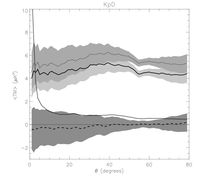
Figure 1: This figure shows the cross correlation function $\langle TM\rangle$ computed from our r1dg-SC template and the V (thick solid line), W (dotted line) and T03 (thick dashed line) CMB maps. Each line is centred in a shaded region limiting the 1-$\sigma$ confidence region computed from Monte Carlo realizations. We associate the high amplitude of the cross correlation for the V & W bands to foregrounds. T03 gives results compatible with zero. The auto correlation function $\langle MM\rangle$ amplified by a factor of 10 is displayed by the thin solid line. Analyses under the Kp2 mask yielded very similar results.

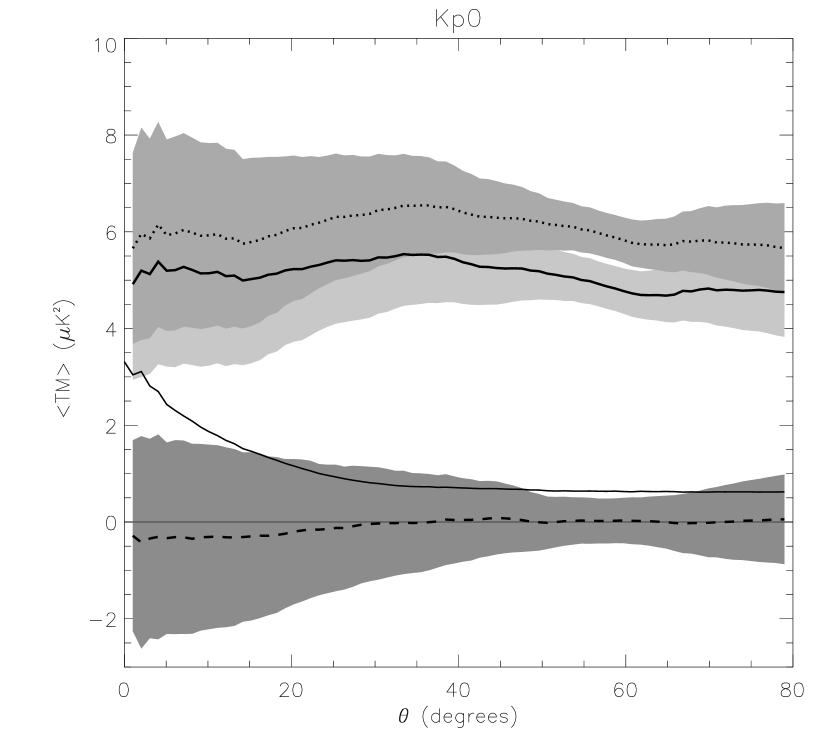
Figure 2: Same as in Fig.(1), but for the Sph-SC template.

6 Discussion and Conclusions

We have used optical (Einasto, APM, ACO) and X-ray based (BCS, NORAS, de Grandi, V98, Vogues) catalogues to locate in the sky tSZ emitting sources as clusters and superclusters of galaxies. Using scaling relations present in the literature, we have assigned microwave fluxes to our sources, and built tSZ catalogues as they would be seen by the W band of WMAP. We have cross correlated these catalogues with WMAP using two different statistical approaches for clusters and superclusters. For the BCS, NORAS and de Grandi cluster catalogues, we claim detections at the 2-5 $\sigma$ level, (except for deGrandi, which gives no detection in the W band). In these cases, we have checked that most of the clusters (and not only the brightest) are contributing to the correlation, with amplitudes of typically 20-30 $\mu$K in the WMAP scans. We fail to detect any statistically significant signal from the (optical) ACO and APM catalogues, (although the latter has chances to give a detection if the noise level decreases after the second year of observations). This may reflect the fact that optical catalogues are not sensitive to the temperature of the IGM in clusters, and might include many clusters that, being present in the optical, contribute with negligible distortions to the tSZ signal, hence diluting the overall cross-correlation. We believe the impact of foregrounds to be of negligible relevance in our results, provided the fact that our method yields very similar results for different masks (Kp0 and Kp2) and different CMB scans, (W band of WMAP and the clean map of Tegmark, de Oliveira-Costa & Hamilton (2003,T03)). Moreover, all these results are recovered when a ring analysis (consisting in studying the temperature fluctuations in annuli centered on cluster pixels) is applied on our catalogues.

With respect to our supercluster templates, we have tested the hypothesis of hot diffuse gas comptonizing the CMB photons in megaparsec scales. We have built two different supercluster templates, depending upon we place the hot gas uniformly in the superclusters or concentrated around the cluster members. By computing the cross correlation function between these templates and the CMB scans, and comparing it with the template auto-correlation function, we have traced the level at which supercluster induced signal is present in the CMB maps. We find that results depend largely on the CMB map we cross-correlate with: the V & W WMAP bands give positive cross-correlation, several $\sigma$-levels above zero. This correlated signal does not vanish when the template is rotated 45 deg in galactic longitude, but drops to zero in the T03 map. The T03 map keeps the same zero temperature level of all bands of WMAP, but combines them in a multipole dependent manner to minimize the presence of foregrounds. Hence, we point to an offset or foregrounds as the most likely responsibles for the different cross-correlation present between our supercluster templates and the W & T03 CMB maps, and we discard the V & W bands from our cross-correlation function analyses. When applying our method ii on T03, we find no significant cross-correlation, and this allows us to place the following constraint on the supercluster induced comptonization parameter $y_{SC}$ associated to the Einasto supercluster catalogues: $y_{SC}<2.18\times 10^{-8}$ at the $2\sigma$ or 95% confidence level. These figures, however, do not account for the uncertainty related to the modelling of the gas distribution. Finally, we conclude noting that any use of the V & W bands in cross-correlation analyses is at best compromised by the presence of a diffuse foreground component, at least at the level of a few microkelvin.

References

- Abell, Corwin & Olowin (1989) Abell, G.O, Corwin, H.G.Jr. & Olowin, R.P. 1989 ApJSS 70, 1
- Banday et al. (1996) Banday, A. J., Gorski, K. M., Bennett, C. L., Hinshaw, G., Kogut, A., & Smoot, G. F. 1996, ApJ 468, L85
- Bennett et al. (2003a) Bennett, C. et al. 2003a ApJ, (accepted)
- Bennett et al. (2003b) Bennett, C. et al. 2003b ApJ, (accepted)
- Bennett et al. (2003c) Bennett, C. et al. 2003c ApJ, (accepted)
- Bennett et al. (1993) Bennett, C. L., Hinshaw, G., Banday, A., Kogut, A., Wright, E. L., Loewenstein, K., & Cheng, E. S. 1993, ApJ 414, L77
- Böhringer et al. (2000) Böhringer, H. et al. 2000 ApJS 129, 435
- Boughn & Crittenden (2003) Boughn, S. P. & Crittenden, R. 2003, astro-ph/0305001
- Boughn & Jahoda (1993) Boughn, S. P. & Jahoda, K. 1993, ApJ 412, L1
- Cooray (1999) Cooray, A. R. 1999, ApJ 524, 504
- Dalton et al. (1997) Dalton, G. B., Maddox, S. J., Sutherland, W. J., & Efstathiou, G. 1997, MNRAS 289, 263
- de Grandi et al. (1999) de Grandi, S. et al. 1999 ApJ 514, 148
- Diego, Silk & Sliwa (2003) Diego, J.M., Silk, J. & Sliwa, W., 2003, astro-ph/0302268
- Ebeling et al. (1996) Ebeling, H., Voges, W., Bohringer, H., Edge, A. C., Huchra, J. P., & Briel, U. G. 1996, MNRAS, 281, 799
- Ebeling et al. (1998) Ebeling, H., Edge, A. C., Bohringer, H., Allen, S. W., Crawford, C. S., Fabian, A. C., Voges, W., & Huchra, J. P. 1998, MNRAS 301, 881
- Ebeling et al. (2000) Ebeling, H., Edge, A. C., Allen, S. W., Crawford, C. S., Fabian, A. C., & Huchra, J. P. 2000, MNRAS 318, 333
- Einasto et al. (1994) Einasto, M., Einasto, J., Tago, E., Dalton, G. B., & Andernach, H. 1994, MNRAS 269, 301
- Einasto et al. (1997) Einasto, M., Tago, E., Jaaniste, J., Einasto, J., & Andernach, H. 1997, A&AS 123, 119
- Fosalba & Gaztañaga (2003) Fosalba, P. & Gaztañaga, E., 2003, astro-ph/0305468
- Ganga, Cheng, Meyer, & Page (1993) Ganga, K., Cheng, E., Meyer, S., & Page, L. 1993, ApJ 410, L57
- Górski, Hivon & Wandelt (1999) Górski, K.M., Hivon, E. & Wandelt, B.D., 1999, Proceedings of the MPA/ESO Cosmology Conference ”Evolution of the Large Scale Structure”, eds. A.J.Banday, R.S.Sheth, and L.Da Costa, PrintPartners Ipskamp, NL, pp.37-42, (also astro-ph/9812350)
- Hogan (1992) Hogan, C.J. 1992 ApJ 398, L77
- Kneissl et al. (1997) Kneissl, R., Egger, R., Hasinger, G., Soltan, A. M., & Truemper, J. 1997, A&A, 320, 685
- Rubiño-Martín, Atrio-Barandela, & Hernández-Monteagudo (2000) Rubiño-Martín, J. A., Atrio-Barandela, F., & Hernández-Monteagudo, C. 2000, ApJ, 538, 53
- Sunyaev & Zeldovich (1980) Sunyaev, R. A. & Zeldovich, I. B. 1980, ARA&A, 18, 537
- Tegmark, de Oliveira-Costa & Hamilton (2003) Tegmark, M., de Oliveira-Costa, A. & Hamilton, A.J.S., 2003, astro-ph/0302496
- Trümper (1993) Trümper, J. 1993, Science 260, 1769
- Vikhlinin et al. (1998) Vikhlinin, A., McNamara, B. R., Forman, W., Jones, C., Quintana, H., & Hornstrup, A. 1998, ApJ 502, 558
- Vogues et al. (1999) Vogues, W. et al. 1999, A&A 349, 389