Strong Gravitational Lensing and Localization of Merging Massive Black Hole Binaries with LISA

Abstract

We study how the angular resolution of LISA for merging massive black-hole binaries would be improved if we observe multiple gravitational wave “images” due to strong gravitational lensing. The correlation between fitting parameters is reduced by the additional information of the second image which significantly reduces the error box on the sky. This improvement would be very helpful for identifying the host galaxy of a binary. The angular resolution expected with multiple detectors is also discussed.

I Introduction

Black holes are a very fascinating prediction of general relativity. Recent observations indicate that massive black holes (MBHs) exist at the centers of many galaxies and their masses have a strong correlation with the properties of their host galaxies Merritt:2001zg . Binary MBHs would be formed by the merger of galaxies that harbor MBHs begelman . The coalescence of such a binary is the most energetic event in the Universe. It finally releases enormous energy (several orders smaller than $c^{5}/G\sim 4\times 10^{59}$erg/sec) over a characteristic time scale $GM/c^{3}\sim 5(M/10^{6}M_{\odot})$sec ($M$: mass of the system). The Laser Interferometer Space Antenna (LISA) can observe gravitational waves from MBH binaries with high signal to noise ratio (SNR) lisa . In the case of equal mass binaries the expected SNR at a given distance is maximum for redshifted masses $\sim 10^{6}M_{\odot}$ and is $\gtrsim 10^{3}$ even at cosmological distances Cutler:1998ta . By fitting the gravitational waves from a MBH binary with templates prepared in advance we can make a stringent test of general relativity and obtain various important data about the black holes (e.g. mass, spin). Therefore gravitational waves from MBH binaries are, by themselves, a very interesting signal for relativistic astrophysics lisa ; Cutler:2002me .

If we can identify their host galaxies, it would also have a significant impact in astrophysics and cosmology. By detailed follow-up observations using electro-magnetic waves at various frequencies we might discover absorbing properties of the galaxies or obtain fundamental clues which will elucidate the evolution of MBHs. In principle, the angular direction of coalescing MBH binaries could be estimated by analyzing data from LISA. Due to annual revolution and rotation of LISA the signal from a MBH binary shows modulation that depends strongly on the ski position of the binary. For equal mass MBH binaries at $z\sim 1$ the angular resolution of LISA would be typically $\sim 10^{-4}$sr for redshifted masses $\sim 10^{6}M_{\odot}$ Cutler:1998ta . The resolution becomes worse for high redshift MBH binaries. The number of bright galaxies is $\sim 10^{4}$ in one square degree ($\sim 3\times 10^{-4}$sr). Therefore the angular resolution of LISA is not sufficient to fully specify the host galaxy of a cosmological MBH binary Cutler:1998ta . Thus an improvement in the angular resolution for a MBH binary would be crucially helpful for selection of candidates for its host galaxy using electro-magnetic telescopes. Possible mechanisms providing such an improvement are worth exploring.

In this context it has been discussed that higher gravitational wave harmonics of Moore:1999zw , precession of the orbital plane in a rapidly spinning system Vecchio:2003tn , or effects caused by LISA’s finite arm-length of Seto:2002uj could become important in some situations. In this paper we show that the angular resolution for a MBH binary could be significantly improved, if we observed multiple “images” of the gravitational waves due to strong gravitational lensing. Our point is not the amplification of the signal but observation of the same source at different epochs. The intrinsic binary parameters such as the chirp mass can be determined very accurately from gravitational waves, so it would not be a hard task to identify two lensed signals from the same merging MBH binary.

If we assume that MBH binaries coalesce shortly after the merger of their host galaxies less than the Hubble time, the hierarchical model of structure formation suggests that the coalescence rate of MBH binaries could be as high as $\sim 100{\rm yr^{-1}}$, and its distribution might be much higher at high redshift than low redshift $z\lesssim 1$ Haehnelt:wt . The probability $\tau$ of strong gravitational lensing also depends strongly on the redshift of the source. At $z\sim 1$ the probability is only $\tau\lesssim 10^{-3}$, but it could reach several percent at $z\sim 5$ Holz:1998uw . Thus we might obtain multiple images (more precisely the chirping gravitational waves) of distant MBH binaries. In this paper it is shown that the additional images caused by lensing with time delay $\Delta T\gtrsim 0.1$yr would greatly decrease the correlations between fitting parameters of the templates, and the angular resolution of a MBH binary could be dramatically improved.

This paper is organized as follows. In Sec II we briefly discuss signal analysis for a single image (IIA) and for multiple images (IIB). Various numerical results are presented in Sec III. We also describe the angular resolution obtained with multiple detectors that are widely separated (IIIC). Our study is summarized in Sec IV.

II Analysis

II.1 Observation of a chirping gravitational wave

The three spacecrafts of LISA maintain a nearly equilateral triangle configuration and move annually around the Sun with the orientation of the triangle changing. As discussed below, the direction of a gravitational wave source can be estimated from the wave signal which is affected by (i) the Doppler effect due to the revolution of the detectors around the Sun and (ii) the amplitude modulation due to the rotation of the triangle and the increase of the wave frequency (chirp signal) lisa ; Cutler:1998ta . For the response of LISA to gravitational waves we follow prince for the time-delay interferometry (TDI) analysis that cancels the laser frequency fluctuations in the data streams Armstrong:uh .

We label three spacecrafts as 1, 2, and 3 and use notation $L_{i}$ ($i=1,2,3$) to denote the length of the arm opposite spacecraft $i$. Information about the binaries is extracted using three data streams $A(t),E(t)$ and $T(t)$ that form an orthogonal basis for the laser-noise canceling combinations. These three data streams are constructed from six (one-way) relative frequency fluctuations $y_{ij}(t)$ ($i,j=1,2,3,i\neq j$) at different times (see prince for explicit expressions of $A,E,T$ in terms of $y_{ij}(t)$). The signal $y_{ij}$ is measured at spacecraft $j$ and transmitted from spacecraft $k(\neq i,\neq j)$ along the arm $L_{i}$.

Our analysis is similar to Cutler:1998ta (see also Vecchio ; Hughes:2001ya ; Holz ). However, as in Seto:2002uj we do not use the long wave approximation which is valid only for incoming gravitational waves larger than the arm-length of LISA $L=5.0\times 10^{6}$km, corresponding to $f=c/2\pi L\sim 0.01$Hz. The study in Seto:2002uj is somewhat incomplete, as the TDI analysis was not included properly. This point is also remedied in this paper. For simplicity we assume that the arm-lengths $L_{i}$ are equal.

First we briefly discuss the gravitational waveform from a MBH binary with a circular orbit. In this paper we only consider the in-spiral waveforms. For larger MBH binaries the contribution of the merger or the ring-down waveforms could be important for SNR Hughes:2001ya . We use the stationary phase approximation and the restricted post-Newtonian approach with 1.5-PN phase Cutler:tc that is given in Fourier space as follows

$$\Psi(f)=2\pi ft_{c}-\phi_{c}-\frac{\pi}{4}+\frac{3}{4}(8\pi Gc^{-3}{\cal M}_{z}f)^{-5/3}[1+\frac{20}{9}\left(\frac{943}{336}+\frac{11\mu_{z}}{4M_{z}}\right)x+(4\beta-16\pi)x^{3/2}],$$ (1)

where $t_{c}$ and $\phi_{c}$ are integration constants, and the former contains information about the coalescence time measured at the Sun not at the detector. The difference between the coalescence times is included in eq.(3). The parameter $\beta$ is the spin-orbit coupling coefficient (we put its true value $\beta=0$), and $\mu_{z}$, $M_{z}$ ${\cal M}_{z}$ are the reduced mass, the total mass and the chirp mass respectively. All of the mass parameters are multiplied by the factor $(1+z)$ ($z$: redshift of the binary) with the suffix $z$. The total mass $M_{z}$ is given by other two masses as $M_{z}={\cal M}_{z}^{5/2}\mu_{z}^{-3/2}$. The post-Newtonian expansion parameter $x=O(v^{2}/c^{2})$ is defined as $x\equiv\left\{G\pi c^{-3}M_{z}f\right\}^{2/3}$.

For simplicity we first consider gravitational waves propagating in a homogeneous background. The effects of lensing will be discussed later. The incoming gravitational wave from a binary is decomposed into plus and cross polarization modes. It is convenient to use the principle axes $({\mbox{\boldmath${p}$}},{\mbox{\boldmath${q}$}})$ defined by the direction ${\mbox{\boldmath${\Omega}$}}_{s}$ and orientation ${\mbox{\boldmath${\Omega}$}}_{l}$ of the binary as ${\mbox{\boldmath${p}$}}={{\mbox{\boldmath${\Omega}$}}_{s}\times{\mbox{\boldmath${\Omega}$}}_{l}}/{|{\mbox{\boldmath${\Omega}$}}_{s}\times{\mbox{\boldmath${\Omega}$}}_{l}|}$ and ${\mbox{\boldmath${q}$}}=-{\mbox{\boldmath${\Omega}$}}_{s}\times{\mbox{\boldmath${p}$}}$. The plus mode has the polarization tensor $e^{+}_{ab}=p_{a}p_{b}-q_{a}q_{b}$ and the cross mode has $e^{\times}_{ab}=p_{a}q_{b}+q_{a}p_{b}$. The relative frequency shift, for example, $y_{31}(t)$, due to these two modes is expressed as

$$y_{31}(t)=\frac{1}{2}(\pi f)^{2/3}\left(\cos 2\psi_{12}A_{+}+i\sin 2\psi_{12}A_{\times}\right)(1-\cos\theta_{12})\left[U(t,1)-U(t-\tau,2)\right],$$ (2)

where $\tau$ is the time $\tau=L/c\sim 17$sec and the function

$$U(t,j)=\exp[-2\pi if(t+{\mbox{\boldmath${x}$}}_{j}\cdot{\mbox{\boldmath${\Omega}$}}_{s}/c)]$$ (3)

describes the phase of the incoming wave at the detector $j$ (with position ${\mbox{\boldmath${x}$}}_{j}$ measured from the Sun) at time $t$. In Eq.(2) we have neglected the very small relative motion of the detectors over the time scale $\tau$ and also the time variation of the frequency over the time scale $1{\rm AU}/c=500$sec. The coefficients $A^{+}$ and $A^{\times}$ are given in terms of an amplitude $A$ as $A^{+}=A(1+\cos^{2}I)$ and $A^{\times}=2A\cos I$ in which $\cos I\equiv{\mbox{\boldmath${\Omega}$}}_{s}\cdot{\mbox{\boldmath${\Omega}$}}_{l}$ is the cosine of the inclination angle. In Eq.(2) $\theta_{jk}$ is the angle between the direction of the binary ${\mbox{\boldmath${\Omega}$}}_{s}$ and the arm ${\mbox{\boldmath${x}$}}_{j}-{\mbox{\boldmath${x}$}}_{k}$, and the principle polarization angle $\psi_{jk}$ is given by $\tan\psi_{jk}=[({\mbox{\boldmath${x}$}}_{j}-{\mbox{\boldmath${x}$}}_{k})\cdot{\mbox{\boldmath${q}$}}]/[({\mbox{\boldmath${x}$}}_{j}-{\mbox{\boldmath${x}$}}_{k})\cdot{\mbox{\boldmath${p}$}}].$ The angles $\theta_{jk}$ and $\psi_{jk}$ change with the motion of the spacecrafts.

The Doppler effects are included in the factor $U(t,j)$. The TDI data streams at time $t$ are constructed from linear combinations of $y_{ij}$ at different times, e.g. $t$, $t-\tau$ or $t-2\tau$. Due to the finite arm-length, the response to gravitational waves shows a complicated behavior that depends strongly on the angular position of the MBH binary. The effect of finite arm-length on the estimation of the source direction could become important around $\sim 10^{5}+10^{5}M_{\odot}$ in the case of equal mass binaries Seto:2002uj . In the long wave limit $f\tau\ll 1$ the above expression (2) is simplified. The analysis by Cutler Cutler:1998ta is essentially in this limit, and the amplitude modulation and phase modulation from Doppler effects can be analyzed separately. As a comparison we also examine the angular resolution of MBH binaries using this method to describe the response of LISA to gravitational waves.

The intrinsic detector noise for a measurement of the fluctuations $y_{ij}$ has two main components that are relevant for the combinations $A,E,T$. They are the proof mass noise and the optical path noise. We use the spectra Armstrong:uh

$$S_{y}^{proof-mass}(f) = 2.5\times 10^{-48}\left(\frac{f}{1\rm Hz}\right)^{-2}{\rm Hz^{-1}},$$ (4)

$$S_{y}^{optical-path}(f) = 1.8\times 10^{-37}\left(\frac{f}{1\rm Hz}\right)^{2}{\rm Hz^{-1}}.$$ (5)

It is a simple task to obtain the noise for the three combinations $A,E,T$. But we note that the detector’s noise below 0.1mHz is somewhat controversial (see e.g. Bender:uv ; Hughes:2001ya ). This frequency region strongly affects our results for larger MBH binaries.

We also include the Galactic binary confusion noise Bender:hs using the following simple approximation

$$S^{Gc}_{h}(f)=\cases{4\times 10^{-37}\left(\frac{f}{1\rm mHz}\right)^{-7/3}{\rm Hz^{-1}}&$(f\leq 10^{-2.7}{\rm Hz})$\cr 0&$(f>10^{-2.7}{\rm Hz})$\cr}$$ (6)

given for one year observation. This confusion noise is about 10 times larger (for $h$) than the detector noise at 1mHz (see figure 5 of prince ). For simplicity we neglect the anisotropies of the Galactic confusion noise in this paper.

We integrate each chirping gravitational wave for 1yr before coalescence up to the cut-off frequency $f_{max}$ when the binary separation becomes $r=6GM_{z}/c^{2}(1+z)$, corresponding to a frequency

$$f_{max}=0.04\left(\frac{M_{z}}{10^{5}M_{\odot}}\right)^{-1}{\rm Hz}.$$ (7)

In contrast the wave frequency $f$ observed at $T$yr before the coalescence time $t_{c}$ is given approximately by

$$f=1.9\times 10^{-4}\left(\frac{{\cal M}_{z}}{0.87\times 10^{5}M_{\odot}}\right)^{-5/8}\left(\frac{T}{1{\rm yr}}\right)^{-3/8}{\rm Hz}.$$ (8)

The signal to noise ratio SNR of a detection is determined by the amplitudes of the modes $A,E$ and $T$ and by the noise spectra $S_{A}(f),S_{E}(f)$ and $S_{T}(f)$ which are constructed from the detector noises (4) (5) and the confusion noise (6). We calculate the signal to noise ratio of the in-spiral waves using thorne ; Finn:1992wt

$${\rm SNR^{2}}=4\sum_{B=A,E,T}\int_{f_{1}}^{f_{min}}\frac{B(f)B^{*}(f)}{S_{B}(f)}df,$$ (9)

where $f_{1}$ is the initial frequency for signal integration. In the present study the number of fitting parameters $\{\alpha_{i}\}$ for each chirping gravitational wave is 10. They are $\{\alpha_{i}\}=\{{\cal M}_{z},\mu_{z},\beta,t_{c},\phi_{c},A,\theta_{s},\phi_{s},\theta_{l},\phi_{l}\}$. Angular variables $(\theta_{s},\phi_{s})$ represent the direction of the binary ${\mbox{\boldmath${\Omega}$}}_{s}$ in a fixed frame around the Sun, and $(\theta_{l},\phi_{l})$ represent its orientation ${\mbox{\boldmath${\Omega}$}}_{l}$. The variance in the parameter estimation errors $\Delta\alpha_{i}$ are evaluated using the Fisher information matrix $\Gamma_{ij}$ as $\left\langle\Delta\alpha_{i}\Delta\alpha_{j}\right\rangle=\Gamma_{ij}^{-1}$ where $\Gamma_{ij}$ is given as Finn:1992wt

$$\Gamma_{ij}=4\sum_{B=A,E,T}\int_{f_{1}}^{f_{min}}\frac{\partial_{i}B(f)\partial_{j}B^{*}(f)}{S_{B}(f)}df.$$ (10)

Following Cutler Cutler:1998ta we use the notation $\Delta\Omega_{s}\equiv 2\pi\sin\theta_{s}\sqrt{\left\langle\Delta\theta_{s}^{2}\right\rangle\left\langle\Delta\phi_{s}^{2}\right\rangle-\left\langle\Delta\theta_{s}\Delta\phi_{s}\right\rangle^{2}}$ for the angular resolution of a binary on the sky.

Our results for the angular resolution $\Delta\Omega_{s}$ change only slightly for masses $\gtrsim 10^{4}M_{\odot}$ when we switch the integration time from 1yr to 10 yr. We put the MBH binaries at $z=3$ in a universe with cosmological parameters $\Omega_{0}=0.3$, $\lambda_{0}=0.7$ (spatially flat universe) and $H_{0}=71$km/sec/Mpc. In this cosmological background the luminosity distance $d_{L}$ becomes $d_{L}=25$Gpc at $z=3$ and $d_{L}=6.5$Gpc at $z=1$.

II.2 Analysis for multiple images by lensing

We discuss parameter fitting of multiple images created by strong gravitational lenses. As we show below the improvement in the angular resolution $\Delta\Omega_{s}$ due to lensed multiple images could be very effective for time delays $\Delta T\gtrsim 0.1$yr. On the other hand a time delay larger than the operation period of LISA (nominally $\sim 3$ yrs, but possibly $\sim$10 yrs) is irrelevant for our analysis. Thus our main targets are multiple images with time delay $0.1{\rm yr}\lesssim\Delta T\lesssim 10$yr. LISA has good sensitivity to gravitational waves with frequency $10^{-4}{\rm Hz}\lesssim f\lesssim 10^{-1}{\rm Hz}$ which is much higher than the inverse of the relevant time delay $(\Delta T)^{-1}\lesssim 3\times 10^{-7}$Hz. We note also that the latter frequency is smaller than $f$ given by eq.(8) for $T=1$yr and ${\cal M}_{z}\lesssim 10^{8}M_{\odot}$. Therefore the geometric optics approximation is valid in our analysis and the structure of phase is not changed by the lensing Nakamura:1997sw ; Takahashi:2003ix . We take the same parameters ${\cal M}_{z},\mu_{z},\phi_{c},\beta$ for the phases eq.(1) of all the multiple images from a source, but the coalescence time $t_{c}$ is, of course, different. In some cases the substructure of the lensing galaxy might complicate the problem Mao:1997ek .

In the case of a homogeneous and isotropic universe the wave amplitude $A$ is given simply in terms of the luminosity distance $d_{L}$ and the chirp mass ${\cal M}_{z}$ by Schutz:gp

$$A_{0}=\frac{2G^{5/3}{\cal M}_{z}^{5/3}}{c^{4}d_{L}}.$$ (11)

The above relation can be used to determine $d_{L}$ from the observed gravitational wave and also to specify the redshift of the binary $z$ by inversion of the $d_{L}$-$z$ relation if the cosmological parameters are known accurately Schutz:gp ; Hughes:2001ya . Note that in general the chirp mass ${\cal M}_{z}$ is determined more accurately than the amplitude $A$ using the time evolution of the gravitational wave phase.

For signals affected by strong lensing we fit different values $A_{i}$ for the amplitude of each image. We cannot apply the above inversion to estimate $z$, but this is not a serious problem for identifying high-z MBH binaries, considering the accumulated effects of weak lensing. At $z\sim 3$ the rms fluctuations of the amplification by weak lensing could become $\sim 0.2$ and hamper the application of the above inversion even for a single image Holz ; Barber:2000pe .

Here we discuss fitting of the angular variables $(\theta_{s},\phi_{s},\theta_{l},\phi_{l})$. First we evaluate the typical image separation for a lensed source. As a model we use the singular isothermal sphere approximation for the density profile of the lensing galaxy. In this model we have the following explicit relation between the image separation angle $\theta$ and the time delay $\Delta T$ lens

$$\Delta T=\frac{\theta^{2}}{2c}\frac{D_{OL}D_{OS}}{D_{LS}}(1+z_{L})y=1.3\left(\frac{\theta}{5^{{}^{\prime\prime}}}\right)^{2}\left(\frac{D_{OL}}{{D_{LS}}}\right)\left(\frac{D_{OS}}{1.4{\rm Gpc}}\right)\left(\frac{1+z_{L}}{2}\right)\left(\frac{y}{0.5}\right){\rm yr},$$ (12)

where $D=d_{L}/(1+z)^{2}$ is the angular diameter distance (e.g. $D_{OL}$: between the observer and the lens), $z_{L}$ is the redshift of the lens, and $y$ is the normalized impact parameter with $y<1$ corresponding to the occurrence of multiple images in the isothermal sphere approximation. The image separation ($\lesssim 5^{{}^{\prime\prime}}$) for the relevant time delay $\Delta T\sim 1$yr is much smaller than the angular resolution of the source direction for cosmological MBH binaries, which will be shown later. This means that we can use the same fitting parameters $(\theta_{s},\phi_{s})$ for the direction of the binary for each image.

The polarization tensor ${\bf e}_{ab}$ of a gravitational wave is parallel transported along a null geodesic gravitation . It is easy to confirm that the directions of the tetrad vectors on a lensed null geodesics change only on the order of the image separation, which is generally much smaller than the resolution of the orientation of a cosmological MBH binary $(\theta_{l},\phi_{l})$. This means that the polarization properties of the multiple images cannot be distinguished observationally and the same fitting parameters $(\theta_{l},\phi_{l})$ can also be used for the orientation of each image.

Let us briefly summarize the number of fitting parameters. For $n$-multiple images from the same source we can take eight common parameters $\{{\cal M}_{z},\mu_{z},\beta,\phi_{c},\theta_{s},\phi_{s},\theta_{l},\phi_{l}\}$, but fit two different ones $\{A_{i},t_{ci}\}$ for each image ($i=1,...,n$). Thus the total number of fitting parameters becomes $8+2n$. In the following analysis we fix the true value of each wave amplitude $A$ (both un-lensed and lensed) by $A=A_{0}$. This would give conservative results for the magnitude of the parameter estimation errors in the case of lensed signals. With our prescription the SNR depends on the total number of images $n$ as $SNR\mbox{\raisebox{-4.30554pt}{$~{}\stackrel{{\scriptstyle\textstyle\propto}}{{\textstyle\sim}}~{}$ }}n^{1/2}$.

III Angular resolutions for MBH binaries

III.1 Basic analysis

We calculate the parameter estimation errors using (i) the TDI method described in Sec II and (ii) the method of Cutler Cutler:1998ta which uses the long-wave approximation. The effective noise curves are somewhat different for these two approaches. In this section various averaged quantities, such as the SNR and the angular resolution $\Delta\Omega$, are evaluated by taking geometrical averages for 100 MBH binaries at $z=3$ with random directions $(\theta_{s},\phi_{s})$ and orientations $(\theta_{l},\phi_{l})$. For simplicity we only study equal mass binaries. The time delay is fixed at $\Delta T=1/3$yr unless otherwise stated.

In Figure 1 the averaged the SNR is presented for redshifted masses $4\times 10^{3}-4\times 10^{8}M_{\odot}$ (true masses $10^{3}-10^{8}M_{\odot}$). Hereafter we mainly use the redshifted mass $m_{z}=m_{1z}=m_{2z}$ to show the mass dependence. When we decrease the mass from $m_{z}\sim 10^{8}M_{\odot}$, the SNR becomes a maximum around $m_{z}\sim 10^{6}M_{\odot}$. This is because the binary confusion noise disappears around $f\sim 10^{-2.7}$Hz in our models and this frequency corresponds to the coalescence frequency $f_{max}$ of a MBH binary with mass $m_{z}\sim 10^{6}M_{\odot}$ as given by eq.(7). The SNR for two lensed images simply increases by a factor of $\sim 1.5\sim\sqrt{2}$ as expected.

In Figure 2 we show the averaged angular resolution as a function of redshifted mass $m_{z}$. For single images the averaged resolution $\Delta\Omega_{1}$ shows weak dependence on the mass for the TDI method, and is nearly constant at $\sim 2\times 10^{-3}$sr for MBH binaries with masses between $m_{z}\sim 10^{5}M_{\odot}$ and $10^{8}M_{\odot}$ at $z=3$. This is a remarkable contrast to Figure 1 for SNR which shows a steep rise around $m_{z}\sim 10^{5}-10^{6}M_{\odot}$. Using the simple method of Cutler we find that the sky positions of a MBH binaries with $m_{z}\gtrsim 10^{5}M_{\odot}$ is mainly estimated from the amplitude modulation due to rotation of the detectors. The Doppler phase modulation has a contribution for $m_{z}\lesssim 10^{5}M_{\odot}$.

When a second image is added by the time delay of lensing, the situation changes drastically. The angular resolution $\Delta\Omega_{2}$ obtained from two images with $m_{z}\sim 4\times 10^{5}M_{\odot}$ is improved by more than two orders of magnitude, compared to a single image $\Delta\Omega_{1}$. The ratio $\Delta\Omega_{1}/\Delta\Omega_{2}$ decreases for both smaller and larger masses. It becomes $\sim 10$ at $m_{z}\sim 10^{4}M_{\odot}$ and $\sim 5$ at $m_{z}\sim 10^{8}M_{\odot}$. This mass dependence is discussed later. We also found that the parameter estimation errors for the intrinsic binary parameters such as the chirp mass would be changed by only a factor of $2$ or so by the second image.

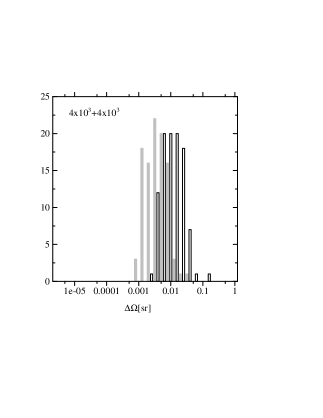
(b)

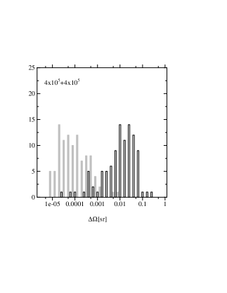
(c)

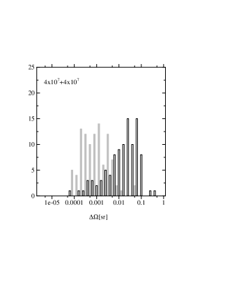
Figure 3: Histograms of the angular resolution $\Delta\Omega_{1}$ (open bars) and $\Delta\Omega_{2}$ (gray bars). The mass $m_{z}$ is fixed at (a) $m_{z}=4\times 10^{3}$, (b) $4\times 10^{5}$ and (c) $4\times 10^{7}$. The results for $\Delta\Omega_{1}$ are displaced by $10^{-0.1}$. The total number of binaries is 100 for each mass. These results were obtained using the TDI method.

In Figure 3 we show histograms of the angular resolutions $\Delta\Omega_{1}$ and $\Delta\Omega_{2}$ in our 100 realizations of MBH binaries with redshifted masses $m_{z}=4\times 10^{3}M_{\odot},4\times 10^{5}M_{\odot}$ and $4\times 10^{7}M_{\odot}$. The impact of lensing is also apparent in these figures.

So far we have fixed the time delay at $\Delta T=1/3$yr. In Figure 4 we present the ratio $\Delta\Omega_{1}/\Delta\Omega_{2}$ as a function of the time delay $\Delta T$. Due to the periodicity in the configuration of LISA, the results obtained for $\Delta T$yr are the same as those for $\Delta T+N$yr with $N$ an integer. As our results are given in the form of a ratio $\Delta\Omega_{1}/\Delta\Omega_{2}$, they do not depend on the distance or redshift to the source as long as we use the redshifted masses. The factor $\Delta\Omega_{1}/\Delta\Omega_{2}$ depends only weakly on the time delay for $\Delta T\gtrsim 0.1$yr.

III.2 Third image

We have also calculated the angular resolution $\Delta\Omega_{3}$ in the case that we could observe a total of three images. We set the two time delays relative to the first image as $\Delta T=1/3$ yr and $\Delta T=2/3$ yr, and fixed the amplitudes of the three images by $A_{0}$ given in eq.(11). The ratios $\Delta\Omega_{1}/\Delta\Omega_{3}$ become $\sim 40$ ($m_{z}=4\times 10^{3}M_{\odot}$), $\sim 800$ ($4\times 10^{5}M_{\odot}$) and $\sim 22$ ($4\times 10^{7}M_{\odot}$). For the first two images analyzed in the previous subsection the ratios $\Delta\Omega_{1}/\Delta\Omega_{2}$ are $\sim 13$ ($4\times 10^{3}M_{\odot}$), $\sim 300$ ($4\times 10^{5}M_{\odot}$) and $\sim 9$ ($4\times 10^{7}M_{\odot}$). Therefore the effect of a third image is not so drastic as that of the second one.

III.3 Multiple detectors

We have shown that the observation of multiple images due to lensing could significantly improve the angular resolution $\Delta\Omega$. But we cannot bet on this passive effect for most merging MBH binaries, considering the probability. In an usual situation we will only detect a single image. Using multiple detectors is one positive method for improving the angular resolution. In this case we can take the same fitting parameters also for the amplitude $A$ and the coalescence time $t_{c}$ (at the Sun). The former is important as the amplitude $A$ and the angular variables will correlate strongly (see eq.(2)). The latter means that we can take advantage of the time delay between the two detectors which is closely related to the direction to the binary.

As a simple extension of our analysis for lensing, we calculate the angular resolution $\Delta\Omega_{II}$ with two detectors that have the same specification as LISA. The two detectors are on the Earth orbit around the Sun as for LISA, but we set the angle between them at $2\pi/3$ corresponding to 1/3yr of orbital time. Thus their distance is fixed at 1AU$\times 2\times\sin(\pi/3)=$1.73AU, and their orientations are always different from each other. For simplicity we assume that the noises in the data streams measured by the two detectors are independent. This would be a valid approximation for the detector noise, but might not be for the binary confusion noise. We evaluate the Fisher matrix using an extension of eq.(2.10) with six data streams; $(A,E,T)$ modes both for the two detectors.

The ratio of angular resolutions for a single LISA $\Delta\Omega_{1}$ and for two LISAs $\Delta\Omega_{II}$ becomes $\Delta\Omega_{1}/\Delta\Omega_{II}\sim 10^{2}$ ($4\times 10^{3}M_{\odot}$), $\sim 6\times 10^{3}$ ($4\times 10^{5}M_{\odot}$) and $\sim 30$ ($4\times 10^{7}M_{\odot}$). Therefore even for binaries at $z=3$ the angular position of a merging MBH binary can be determined with error box $\sim 10^{-6}$sr, namely (several arc-minutes)². This area on the celestial sphere is close to the resolution obtained from Gamma-Ray-Bursts for determining their host galaxies. When another detector (a total of three) is added with positions characterized by 1/3yr and 2/3yr, the ratio $\Delta\Omega_{1}/\Delta\Omega_{III}$ becomes $\sim 400$, $\sim 4\times 10^{4}$ and $\sim 60$ respectively.

III.4 Effective time

As shown above, the angular resolution $\Delta\Omega$ could be improved significantly for $m_{z}=10^{5}\sim 10^{6}M_{\odot}$. Here we analyze this mass dependence. Roughly speaking, the SNR characterizes the magnitude of the Fisher matrix $\Gamma_{ij}$ as we can understand from eqs.(9) and (10). When the correlation (degeneracy) between the fitting parameters is large, the parameter estimation errors such as $\Delta\Omega$ also become large. This correlation depends strongly on the configuration of LISA around the epoch when the SNR accumulates. In this situation some independent information e.g. added by the second image, has an important role in reducing the correlation and improving the angular resolution $\Delta\Omega$. This fact can be anticipated by comparing Figures 1 and 2.

The angular directions of MBH binaries are mainly estimated from the amplitude modulation and the Doppler phase modulation caused by the revolution and rotation of LISA. A long duration observation is crucial for determining them well. Therefore the correlation between parameters including the direction would be related to the effective observational period, and a binary with a shorter observational period would have a larger ratio $\Delta\Omega_{1}/\Delta\Omega_{2}$. Let us define a time $t_{eff}$ by weighting the time before coalescence $t_{c}-t$ by the amplitude of the wave $h(f)$ and the noise curve $S_{h}(f)$ as follows

$$t_{eff}^{2}\equiv\frac{\left(4\int\frac{h(f)h^{*}(f)(t-t_{c})^{2}}{S_{h}(f)}df\right)}{\left(4\int\frac{h(f)h^{*}(f)}{S_{h}(f)}df\right)}.$$ (13)

Here we formally wrote down the above expression (see eq.(9)). The denominator is nothing but the square of the SNR. As the weight factor $|h(f)|/S_{h}(f)^{1/2}$ does not have a very spiky structure, we can regard $t_{eff}$ as an effective observational period of the binaries. For monochromatic sources we have $t_{eff}=1/\sqrt{3}$yr. In figure 5 we show the time $t_{eff}$ (solid curve) and the ratio of the angular resolution $\Delta\Omega_{2}/\Delta\Omega_{1}$ (dashed curve). The overall shapes of the curves are similar as expected.

The mass dependence of $t_{eff}$ can be understood as follows. For larger mass binaries with $m_{z}\gtrsim 10^{5}M_{\odot}$, the SNR (denominator of eq.(13)) comes mainly from the wave emitted close to the final coalescence. But these waves have a small contribution to the numerator. A binary with mass $m_{z}\lesssim 10^{6}M_{\odot}$ has coalescence frequency larger than $10^{-2.7}$Hz, which is critical for the Galactic binary confusion noise. Therefore the effective observational time $t_{eff}$ decrease significantly for $m_{z}\lesssim 10^{6}M_{\odot}$. The smaller mass ($m_{z}\lesssim 10^{4}M_{\odot}$) binaries stay in the sensitive frequency region for a longer time, and the effective time $t_{eff}$ increases.

IV summary

In this paper we have studied how the angular resolution of LISA would be improved if we observe multiple images due to strong gravitational lensing. It is found that the error box on the sky could be typically 100 times smaller for redshifted mass $m_{z}=10^{5}\sim 10^{6}M_{\odot}$. The improvement in the angular resolution depends strongly on the masses of the MBH binaries. This mass dependence can be roughly explained by using an effective observational time for the binary.

We have mainly discussed the effects of lensing on the matched filtering analysis of gravitational waves, but lensing would also be of great advantage in searching for the host galaxy of a MBH binary using electro-magnetic waves. Besides the fact that the target itself is lensed, additional information obtained from the gravitational waves, such as the time delay or the ratio of the amplification factors of the images, could be used to specify the host galaxy.

We have also calculated the angular resolution expected for multiple detectors and found that the resolution could be improved by a factor of $\sim 6\times 10^{3}$ ($m_{z}\sim 4\times 10^{5}M_{\odot}$) compared to that from a single detector. If LISA could detect gravitational waves from MBH binaries, very exciting results might be obtained by launching another detector.

Figure 1: Averaged SNR for equal mass binaries at $z=3$. The thick curves are for the TDI method and the thin ones are for the method of Cutler. The results for the single (double) image are given by the dashed (solid) curves respectively. The horizontal axis represents the redshifted mass $m_{z}$.

Figure 2: Averaged angular resolution. The identification of each curve is the same as in figure 1.

(a)

Figure 4: Averaged ratio $\Delta\Omega_{1}/\Delta\Omega_{2}$ as a function of the time delay $\Delta T$. The three curves represent different masses. These results do not depend on the distance to the binaries. The TDI method was used again.

Figure 5: The effective time $t_{eff}$ (solid curve: left axis) and the ratio $(\Delta\Omega_{1}/\Delta\Omega_{2})^{-1}$ (dotted curve: right axis) as functions of the redshifted mass $m_{z}$. The TDI method was used here again.