Non-spherical evolution of the line-driven wind instability

Abstract

In this paper, we study the structure and stability of line driven winds using numerical hydrodynamic simulations. We calculate the radiation force from an explicit non-local solution of the radiation transfer equation, rather than a Sobolev approximation, without restricting the flow to one-dimensional symmetry. We find that the solutions which result have complex and highly variable structures, including dense condensations which we compare to observed variable absorption features in the spectra of early type stars.

1 Introduction

The winds of hot, luminous, early-type stars are composed of material photoionized by the bright ultraviolet continuum of the star. Lucy & Solomon (1970) proposed that resonance line scattering by metal ions would provide a strong source of driving, to explain the high mass-loss rates and flow velocities observed. While a single resonance line of gas at rest would only be driven by a small part of the stellar spectrum, the many ($\approx 10^{3}$) resonance lines and the variation of the line frequency which results from the Doppler shift multiply the line force until it dominates other driving mechanisms.

Detailed calculations can be made in which an accurate line-list is used and radiative transfer is calculated using a photospheric spectral energy density distribution, but the computational expense required necessitates other approximations and the accuracy of the results depends on the accuracy of the line-list used. Castor, Abbott and Klein [Castor et al. 1975] (hereafter CAK) proposed an alternative approach, where instead of using a detailed table of line opacities, the force is calculated assuming a distribution function of the numbers of lines present as a function of the line opacity, generally specified as a power-law (indeed, the results of more detailed studies are often characterised in terms of an effective power-law parameter). CAK use the large-velocity gradient approximation (Sobolev 1960) to allow the steady-state structures of the winds to be determined by integration of a simple ordinary differential equation.

The Sobolev approximation is more suitable in a steady state model than for a time-dependent simulation, since effects that evolve on a small scale will not be adequently accommodated. This issue was addressed by Owocki, Castor and Rybicki [Owocki et al. 1988] (hereafter OCR) where the Sobolev approximation is replaced by an explicit calculation of the optical depth. In this paper, they use what they term a pure-absorption approximation, in which photons which interact with the gas are removed from the stellar spectrum. While this initially seems a strange approach to modelling a wind driven predominantly by resonance scattering, the frequency redistribution (in the rest frame of the star) achieved in the scattering process means that it is a reasonable first approximation, and indeed the accuracy of the results obtained have been confirmed by subsequent, more detailed, studies by the same authors.

In the present paper, we apply the pure-absorption approximation of OCR to study the local structure and stability of line-driven winds. This work complements previous studies, which have generally either used the non-Sobolev treatment pioneered by OCR [Owocki 1991, Owocki & Puls 1996, and further developed by], but been restricted to spherical symmetry, or sacrificed the non-local treatment of the radiation field to allow the flow to be studied in higher dimensionalities. In common limiting cases, our results agree with these other models to reasonable accuracy. When a non-local treatment of the radiation transfer is combined with integration in a two-dimensional domain, features result which are entirely novel. An initial effort to move into the two dimensional domain was considered by Owocki (1999), where they consider a multiple ray approach to the calculation of the line driving.

The plan of this paper is as follows. In Section 2 we discuss the physical basis for a line driven from the Sobolev, CAK and OCR formalisms. In Section 3 we discuss an approximate method for the solution of the line driving force, the initial conditions used and introduce three statistical parameters for use in analysing the results. In Section 4 we introduce a 1D model, which can be compared to previous calculations. The evolution of different sizes of perturbation are considered, the data is statistically analysed and the absorbtion spectrum is calculated. In Section 5 the 1D model is extended to a 2D model and the resulting structure is discussed. A summary is presented in Section 6.

2 Radiative force and Hydrodynamics

The absorption and scattering of radiation is the dominant process which drives hot star winds. The interaction of stellar photons with wind particles accelerate the particles away from the star. Treated in full generality, the combined problem of hydrodynamics and radiation transfer is a highly coupled integrodifferential system. However, OCR demonstrated that a pure absorption model gave a reasonable account of the local dynamics of wind instabilities in spherical symmetry. In this paper, we study the flow of gas in less symmetrical situations, and adopt the pure absorption model as a tractable first approximation.

The general expression for monochromatic optical depth in a wind is

$$\tau_{\nu}(r)=\int^{r}_{0}\rho(r^{\prime})\kappa_{\nu}(r^{\prime})dr^{\prime},$$ (1)

where $\rho(r)$ is the density of the gas at a distance $r$ from the photosphere and $\kappa_{\nu}$ is the opacity at frequency $\nu$, per unit mass of the wind material. For a single absorption line, this can be expressed in terms of a profile function,

$$\tau_{\nu}(r)=\int^{r}_{0}\rho\kappa_{\rm l}\phi\left(x(\nu)-\frac{v(r^{\prime})}{v_{\rm th}}\right)dr^{\prime},$$ (2)

where $x$ is the frequency displacement from line centre for gas at rest with respect to the star, in units of the line width, $\Delta\nu$,

$$x=\frac{\nu-\nu_{0}}{\Delta\nu},$$ (3)

and $\Delta\nu=(v_{\rm th}/c)\nu_{0}$ when the line width is dominated by thermal broadening. The lines are Doppler shifted by the local velocity, $v(r)$ of the stellar wind.

The profile function, $\phi$, gives the relative likelihood that a photon will be scattered as a function of the offset of the frequency of the photon from line-centre in the local rest frame of the gas. It is given as a function of $x$, normalised so that

$$\int_{-\infty}^{\infty}\phi(x)dx=1$$ (4)

so $\kappa_{\rm l}$ is the line opacity integrated over the line profile divided by the the line width, $\Delta\nu$ (and so for a specific state of the wind material, $\kappa_{\rm l}v_{\rm th}$ is independent of $v_{\rm th}$). The line profile is determined from a combination of intrinsic (quantum) line width, thermal motion and pressure broadening. For conditions which apply in a stellar wind, it may be taken as Gaussian with a thermal width, although the Lorentzian wings may be an important factor at the base of the wind [Poe et al. 1990]. The variation of line profile between ions is small enough to be neglected in the present work. The role of photospheric Lorentz wings in wind acceleration in B stars was investigated by Babel (1996).

Following OCR, the acceleration due to a line at a particular frequency, $\nu_{0}$, and opacity $\kappa_{\rm l}$, can be expressed as,

$$g_{\nu_{0},\kappa_{\rm l}}=\frac{\kappa_{\rm l}v_{\rm th}\nu_{0}F_{\nu_{0}}}{c^{2}}\int_{-\infty}^{\infty}dx\;l_{0}(x)e^{-\tau(x,r)}\phi\left(x-\frac{v(r)}{v_{\rm th}}\right),$$ (5)

where the factor preceding the integral,

$$g_{\rm thin}=\frac{\kappa_{\rm l}v_{\rm th}\nu_{0}F_{\nu_{0}}}{c^{2}},$$ (6)

is the line acceleration in the optically-thin limit. The function $l_{0}(x)$ is the photospheric profile of the line, so that

$$F_{\nu_{0}}(r)=F_{\nu_{0}}l_{0}(x)e^{-\tau(x,r)}$$ (7)

gives the strength of the local radiation field at position $r$ and offset $x\Delta\nu$ from the line centre $\nu_{0}$.

In a stellar wind, there are many ionic transitions with different frequencies and line strengths. Rather than treat this ensemble of lines in detail, CAK developed a statistical approach based on a power law distribution line number density as a function of opacity. OCR extended this model, by assuming that the line opacities were distributed as

$$N(\kappa)={1\over\kappa_{0}}\left(\kappa\over\kappa_{0}\right)^{\alpha-2}\exp(-\kappa/\kappa_{\rm max}),$$ (8)

including an exponential cutoff at large opacity. Assuming that the underlying continuum radiation is approximately constant over the line absorption band, the radiation acceleration from the ensemble of lines is given by

$$g_{\rm rad}(r) = \frac{N_{0}F\Gamma(\alpha)}{c}\left(\frac{v_{\rm th}}{c}\right)^{\alpha}$$ (9)

$$\times \int^{\infty}_{-\infty}dx\frac{\phi(x-v(r)/v_{\rm th})}{(\eta(x,r)+1/\kappa_{\rm max}+\phi(x)/\sigma_{c})^{\alpha}}\;,$$

where $\eta(x,r)$ is the ratio of the optical depth to the opacity and can be thought of as a profile weighted column density from the photosphere to a point $r$ in the wind,

$$\eta(x,r)=\frac{\tau(x,r)}{\kappa_{\rm l}}=\int^{r}_{r_{*}}dr^{\prime}\rho(r^{\prime})\phi\left(x-\frac{v(r^{\prime})}{v_{\rm th}}\right).$$ (10)

As indicated by OCR, a useful way of determining the radiation force, equation (9), is to use differences of its integral, the radiation pressure

$$\rho g_{\rm rad} = \frac{d(P_{rad})}{dz}$$ (11)

$$P_{\rm rad} = -\frac{N_{0}F\Gamma(\alpha)}{(1-\alpha)c}\left(\frac{v_{\rm th}}{c}\right)^{\alpha}$$ (12)

$$\times \int_{-\infty}^{\infty}dx\left[\eta(x,r)+\frac{1}{\kappa_{\rm max}}+\frac{\phi(x)}{\sigma_{c}}\right]^{1-\alpha}\;.$$

The above neglects the effects of re-emitted or scattered radiation. One important such effect is the ‘line-drag’ phenomenon, described by Lucy (1984). This can prevent small-scale velocity perturbations from growing as a result of the anisotropic scattered radiation field. While we neglect this effect in the present work, we discuss how our methods may be extended to take account of its influence.

2.1 The Sobolev approximations

In the limit of narrow lines, the profile function reduces to a delta function and the integral in equation (10) can found analytically, giving

$$\tau_{\nu}=\sum_{r_{i}}\kappa_{\rm l}v_{\rm th}\rho(r)\left|\frac{dv}{dr}\right|^{-1},$$ (13)

where the sum is over the positions, $r_{i}$, at which the line of interest is Doppler shifted to frequency $\nu$. This will only occur once in a monotonically accelerating wind with a single line, and is often assumed to only occur once in simple treatments of more general flows. This is known as the Sobolev, or large velocity gradient, approximation.

The local radiation driving for a single optically thick line is then given by

$$g_{\rm Sob}=\left(\frac{\nu F_{\nu}}{cv_{\rm th}\rho}\right)\left|\frac{dv}{dr}\right|.$$ (14)

For an ensemble of lines obeying the distribution function (8), OCR find

$$g_{\rm Sob}={N_{0}F\Gamma(\alpha)\over(1-\alpha)c}\left({1\over\rho c}\left|dv\over dr\right|\right)^{\alpha}\left[(1+\tau_{\rm max})^{1-\alpha}-1\over\tau_{\rm max}^{1-\alpha}\right],$$ (15)

where

$$\tau_{\rm max}\equiv{\rho\kappa_{\rm max}v_{\rm th}\over|dv/dr|},$$ (16)

which gives the CAK acceleration $g_{\rm CAK}$ in the limit $\kappa_{\rm max}\to\infty$.

The ratio of the thermal velocity to the velocity gradient, $\ell_{\rm Sob}=v_{\rm th}/|dv/dr|$, is called the Sobolev length. This is the length scale over which the flow velocity increases by a thermal velocity. The Sobolev approximation is invalid when velocity gradients are small and cannot be used to study the dynamics of processes with length scales smaller than the Sobolev length.

3 Numerical method

We performed numerical simulations of line-driven winds using the code vh-1 (Blondin 1990). This code uses the Piecewise Parabolic Method (PPM) of Colella & Woodward [Collela & Woodward 1984] to solve the equations of hydrodynamic grid, using Lagrangian coordinates to advance the solution, which is then re-mapped onto an Eulerian grid.

We added an additional force corresponding to line driving by a radiation field. The derivation of this force term is described in detail in the following section. The gas is assumed to be isothermal. We treat the flow relatively far from the photosphere, which allows us to use plane-parallel symmetry and to ignore finite disc effects and spherical divergence, but requires that the wind velocity is everywhere supersonic.

The scaling of the problem is kept arbitrary in the present paper, since we are interested in the general behaviour of line-driven winds. As a result, our results are not restricted to particular stellar parameters. The dimensionless parameters which must be specified include the ratio of the thermal velocity to isothermal sound speed, which we choose to be $v_{\rm th}/c_{\rm s}=0.5$ [Poe et al. 1990]. This is the maximum value which produces a stable flow and is still physically plausible. Lower values of this ratio are inclined to create a less steep and more unstable flow.

We take the boundary conditions to be constant velocity and density at the inner boundary and free outflow at the outer boundary throughout, with reflective boundary conditions at the sides of the two-dimensional simulations. The size of the numerical grid was kept constant, $800$ cells for one-dimensional simulations and $800\times 200$ for two dimensions.

The value of the CAK power-law line-ensemble index is fixed at a typical value of $\alpha=0.7$ (OCR).

3.1 Optical depth calculation

The calculation of the radiation force, equation (12), for a particular cell reduces to differencing the values of the radiation pressure at the interfaces of the cell,

$$P^{i}_{rad}\propto\int^{x_{1}}_{x_{2}}dx\left[\eta(x,r)+\frac{1}{\kappa_{\rm max}}+\frac{\phi(x)}{\sigma_{c}}\right]^{1-\alpha},$$ (17)

where $\eta(x,r)$ is the profile weighted column density which is the amount of radiation absorbed by the wind up to the point $r$. The direct calculation of the double integral implicit in this equation can dominate the time for a computation.

However, since the radiative driving force is dependent not on the radiation pressure but rather on its gradient, a local approach can be taken. At any position the transmitted spectrum will only change over a small range of offsets $x$ around the value for the local mean flow, and the radiation driving will be obtained from the momentum of just these absorbed photons. The force calculation can therefore be speeded up considerably by storing the local scaled optical depth $\eta(x)$, and advancing it by a short-characteristics method. Only the value of the previous spectrum step, $\eta_{i-1}$, and the increase across the current cell $\Delta\eta_{i}$ are necessary to calculate the driving force in cell $i$,

$${dP_{\rm rad}\over dz}=\sum_{n=x_{1}}^{x_{2}}[(\eta_{n}+1/\kappa_{\rm max})^{1-\alpha}-(\eta_{n-1}+1/\kappa_{\rm max})^{1-\alpha}]\Delta x.$$ (18)

Using the quantity

$$\eta(x,r)^{\star}=\eta(x,r)+\frac{1}{\kappa_{\rm max}}+\frac{\phi(x)}{\sigma_{c}}$$ (19)

in our numerical calculations allows the photospheric profile and opacity limit to be absorbed in the initial conditions. In fact, we also neglect the reversing layer term, since the physical domain is assumed to be far away from the photosphere.

3.2 Choice of profile function

In the present paper, we approximate the profile function by a top hat function. This allows the calculation of the increase in column density to further simplified, by using the analytic formulae for the convolution of this function with the column density profile within the grid cell,

$$h_{i}(v)=\left\{\begin{array}[]{ll}\rho_{i}\Delta x_{i}/(v_{\rm u}-v_{\rm d})&v_{\rm d}<v<v_{\rm u}\\ 0&\mbox{otherwise,}\\ \end{array}\right.$$ (20)

$$\Delta\eta_{i}=\phi_{i}\otimes h_{i},$$ (21)

where we have taken the density to be constant within grid cell and the velocity vary linearly between limits $v_{\rm d}$ and $v_{\rm u}$ at its edges. While these distributions differ from the profiles assumed in the hydrodynamical solution, we are free to assume this in the spirit of operator splitting. As we shall see, the results are sensitive to the way in which the velocity limits for the cells are determined from the cell-centred values in the hydrodynamical solution.

In reality, it would be more appropriate to take the line profile function to be a thermal Doppler function or Voigt profile. However, our approximation should not have too dramatic an effect on the results. Owocki & Rybicki (1984) compare the effect of different forms of the profile function with analytical asymptotic solutions, for the ratio of the perturbed line force, $\delta g$ to the perturbed velocity, $\delta v$. They operate the line driving on a sinusoidal velocity perturbation of the form

$$\delta v(z)=\delta v_{0}e^{ikz},$$ (22)

where $\delta v_{0}$ is the velocity perturbation that propagates along with the mean flow of the wind, $k$ is the wavenumber of the perturbation, and $z$ is the Cartesian distance away from the photosphere. A useful quantity to determine is the ratio of the perturbation of the acceleration to the apploed velocity perturbation, $\delta g/\delta v$. Owocki & Rybicki (1984) show that if this quantity has a positive real part, the flow is unstable.

When the optical depth within a Sobolev length is large, $\tau_{0}=\rho_{0}\kappa_{\rm l}\ell_{\rm Sob}\gg 1$, a top hat profile gives an analytic solution matching the asymptotic forms

$$\frac{\delta g}{\delta v}\approx\omega_{0}\frac{ik}{\chi_{0}+ik},$$ (23)

where $\chi_{0}=\rho_{0}\kappa$ is the line strength in the mean flow, and $\omega_{0}=g_{\rm thin}/v_{\rm th}$ is the growth rate of perturbations in the short-wavelength limit, and the growth rate decreases to zero for long-wavelength perturbations.

In the optically thin limit, $\tau_{0}\ll 1$, this ratio becomes,

$$\frac{\delta g}{\delta v}\sim\tau_{0}$$ (24)

which is independent of the wavenumber and solely dependent on the optical depth. This tends to zero making the perturbed acceleration negligible.

By this perturbation analysis it is clear that while the flow feature remains optically thick the flow will be stable. This is shown in equation (23) where only the phase of the initial perturbation is affected by a change in the acceleration. In the limit of short wavenumber perturbations, $\lambda\gg\ell_{\rm Sob}$ the perturbed force reduces to the Sobolev approximation $\delta g\sim\delta v^{\prime}$. The evolution of an optically thin perturbation, equation (24), is unstable since a change in the velocity field produces a change in the acceleration. Since there is no wavenumber dependence of the force in equation (24) the acceleration will continue until the perturbation becomes optically thick.

The form of the profile function will have no effect on the radiation driving force on scales larger than the Sobolev length. As we find (and as has been seen in previous work), the growth of instabilities soon leads to smooth flow regions which are separated by strong shocks and high-gradient rarefactions in which the Sobolev length will not be resolved by the numerical grid. In these latter regions, discretisation errors in the hydrodynamical scheme will probably be at least as important as errors due to our approximation to the line profile function, and so it seems reasonable to use this computationally convenient form in this first treatment.

While we have argued that the top hat-profile function is adequate for use in this initial calculation, we will in future work extend this to more realistic forms. The generalisation may be achieved by representing the profile using a sum of top hat functions, or with a higher order approximation.

As a final word of justification to the use of a top-hat function in this approximate wind solution we present a comparison of our top-hat model with preliminary results using a Gaussian profile. We defer a full comparison of the numerical effects of different profile shapes to future work, so as not to detract from the main thrust of the current paper. We compare results for the different profile functions in two limits, (i) absorption due to a wind with constant velocity gradient and constant density, (ii) absorption due to a data set, representative of a wind solution containing small scale structure. As can be seen from Fig. 1 there is little discernible difference between the two approaches. These preliminary tests indicate that the use of a top-hat function is not a serious over simplification in the limits of this numerical implementation. We do acknowledge that the Gaussian form of the profile function is a large improvement over the top-hat and for future models where smaller length and velocity scales are resolved, it should be used.

(i)

(ii)

Figure 1: These plots show the acceleration from wind solutions using (i) constant density, $\rho=1$ and constant velocity gradient, $\Delta v/v_{\rm th}=0.25$, $\Delta x=0.05$ (ii) a driven flow which contains structure, including shocks (cf. § 4.2.1). The Gaussian model curve (dashed) is overlaid on to the top-hat model curve (solid). The structure is very similar although the Gaussian example does produce a smoother acceleration profile for the case where there is much structure in the wind. The acceleration amplitude is given in code scaled units and are intended to illustrate the similarities between the two methods.

3.3 Initial conditions

We at first used a solution of the steady-state CAK equations to provide initial conditions for our simulations. However, it was found that the change to a discrete grid resulted in significant disturances in the subsequent flow solutions. Instead, we ran the code without perturbations and took the output data set as the starting point for subsequent simulations.

We use constant velocity ($v=1$) and density ($\rho=1$) as the inner boundary condition. The radiation incident at the inside of the grid was assumed to be a unabsorbed pure continuum. Since the flow considered here is supersonic at the outset, it is not consistent to use a photospheric profile, as assumed by OCR. As a result, there is a narrow adjustment layer where the radiation field is first absorbed, but this does not change the overall mass flux through the simulation. It will, of course, be important to include the photospheric profile in future work, when we include the geometric divergence of the flow and calculate the development of the wind from the photosphere outwards.

The values of the code units used throughout this work are shown in Table 1. Although arbitrary code units are used in the numerical simulations, using typical physical values [Owocki et al. 1988] of parameters (listed in Table 1), the length units used here are equivalent to stellar radii.

Code Parameter	Value
$v_{\rm th}/c_{\rm s}$	0.5
$\alpha$	0.7
$\kappa_{\rm max}$	$10^{4}$
Physical Parameter	Value
$v_{\rm th}$	$40{\rm kms^{-1}}$
$\rho_{0}$	$10^{-11}{\rm gcm^{-3}}$
$N_{0}$	$10.15{\rm(cm^{2}g^{-1})^{1-\alpha}}$
$F$	$1.48\times 10^{14}{\rm gs^{-3}}$

Table 1: Code and physical parameter values

3.4 Statistical descriptors of the flow

As suggested by Runacres & Owocki [Runacres & Owocki 2002], the time-dependent flow of the wind can usefully be characterized by three statistical parameters: the clumping factor, velocity dispersion and correlation function. These give an indication of the mean level of flow fluctuations at different points, and the form that these take. In particular, the clumping factor will be unity and the velocity dispersion will be zero in regions where the density varies little with time, and significantly larger if the density has strong transient features. The correlation coefficient indicates if the velocity and density are in (out) of phase, corresponding to a dominance of forward (reverse) shocks in the flow, strong (anti) correlation is shown when C $\rightarrow+(-)1$.

The clumping factor, velocity dispersion and correlation coefficient are calculated using the relations

$$f_{{\rm cl},i} = \frac{\langle\rho_{i}^{2}\rangle}{\langle\rho_{i}\rangle^{2}},$$ (25)

$$v_{{\rm disp},i} = \sqrt{\langle v_{i}^{2}\rangle-\langle v_{i}\rangle^{2}},$$ (26)

$$C_{v\log\rho,i} = \frac{\langle v_{i}\log\rho_{i}\rangle-\langle v_{i}\rangle\langle\log\rho_{i}\rangle}{v_{\rm{\rm disp},i}\sqrt{\langle(\log\rho_{i})^{2}\rangle-\langle\log\rho_{i}\rangle^{2}}},$$ (27)

where the angle brackets refer to a time average of flow quantities in cell $i$; the parameters are functions of the position at which the time average is calculated. (The values were calculated only using discrete samples in the evolution of the simulations, so in practice we also extended the average over finite spatial regions to remove spurious numerical noise.)

4 One-dimensional simulations

In this section, we describe one dimensional simulations using a variety of forms for the radiation driving force. We present these in order to allow comparison of our results with those of previous authors. The simulations were performed both using a local driving force, based on the CAK formalism, and using the pure absorption approximation.

Previous studies, for example by Gayley et al. [Gayley et al. 2001] and Proga et al. [Proga et al. 1998], have applied local radiation driving terms to flows in binary stellar systems and from the surface of accretion discs. We find here that the results so obtained are crucially dependent on the manner in which the flow velocity gradient is determined.

We then present the one-dimensional results of our treatment of the pure absorption approximation. The behaviour of an unperturbed flow has been studied by many different authors (e.g. OCR, Runacres & Owocki [Runacres & Owocki 2002]). The basic stuctures of line driven flows are rarefactions, steep reverse shocks as fast upstream material runs into slow downstream material and de-shadowing of downstream gas, where gas recieves an increase in acceleration from the radiation field as it moves with sufficient velocity so that the incident radiation no longer lies in the range that is absorbed by the upstream patch. We find good agreement with these results. We then study the development of flows with small and large perturbations.

4.1 CAK force law

The radiation force may be calculated as a function of purely local conditions using the CAK formalism. As described above, this leads to an acceleration term given by equation (15) in the limit $\tau_{\rm max}\to\infty$, that is

$$g_{\rm CAK}=\frac{N_{0}F\Gamma(\alpha)}{(1-\alpha)c}\left(\frac{1}{c\rho}\left|\frac{dv}{dr}\right|\right)^{\alpha}.$$ (28)

This has a milder dependence on velocity gradient than that given by equation (14), as a result of allowing for the effect of locally optically-thin lines.

In order to implement the CAK driving force, a form of differencing has to be chosen for the velocity gradient. We investigate here two extreme cases. The upstream form is defined as

$$\frac{\Delta v_{\rm u}}{\Delta r}\rightarrow\frac{v_{n}-v_{n-1}}{r_{n}-r_{n-1}},$$ (29)

and downstream form with

$$\frac{\Delta v_{\rm d}}{\Delta r}\rightarrow\frac{v_{n+1}-v_{n}}{r_{n+1}-r_{n}}.$$ (30)

The choice of differencing direction determines the direction in which information is propagated by the radiation force term. The upstream calculation implies that the force depends on the gas properties in the current and the previous cells. In the downstream case, by contrast, gas can ‘see’ material in its shadow, which does not correspond to the underlying physics of the radiation flow (at least in the absence of scattering).

In Fig. 2, we compare the results of simulations using these two forms. We find that the downstream method, equation (30), method is stable, and recovers the solution of the steady-state CAK equations with good accuracy. When the flow is highly supersonic, the steady-state momentum equation becomes

$$v{dv\over dr}=g_{\rm CAK},$$ (31)

and since the mass flux $\Phi=\rho v$ is constant, $g_{\rm CAK}\propto(v|dv/dr|)^{\alpha}$. As a result, the velocity increases as $v\propto(r-r_{0})^{1/2}$, which is a good approximation to the form of the solid curve in Fig. 2.

However, the flow calculated using the upstream method, equation (29), is unstable. If a stable steady flow is obtained using the downstream method it will become unstable at every point, when the method is changed to upstream calculation. This instability is not a short lived phenomenon but persists as long as the upstream method is used. This suggests that the instability is an intrinsic property of the form of radiation driving law used, rather than simple the result of initial flow perturbations and boundary effects sweeping across the grid.

Figure 2: Instability in the wind produced by changing the direction of velocity calculation. Dashed curve shows upstream gradient and solid shows downstream. Both curves use the CAK radiation driving force law.

This behaviour may be understood in terms of the propagation of ‘Abbott waves’. Abbott (1980) treated the propagation of flow perturbations in the Sobolev limit. In one dimension, he found 2 radiative-acoustic wave modes moving at speeds

$$v_{-} = v-{1\over 2}f_{\rm L}^{\prime}-\sqrt{\left({1\over 2}f_{\rm L}^{\prime}\right)^{2}+c_{\rm s}^{2}}$$ (32)

$$v_{+} = v-{1\over 2}f_{\rm L}^{\prime}+\sqrt{\left({1\over 2}f_{\rm L}^{\prime}\right)^{2}+c_{\rm s}^{2}},$$ (33)

where $f_{\rm L}^{\prime}$ is the derivative of the radiation force with respect to the velocity gradient. The critical points in the steady-state CAK equation occur where one or other of these mode velocities is zero.

The first of these radiative-acoustic modes is, however, somewhat mysterious, as it moves upstream through the flow at a speed faster than the sound speed in the gas. Owocki et al. (1986) demonstrated that Abbott’s approach is justified only for purely wave-like modes, in which the structure of the entire perturbation can be analytically continued from any finite part of it. This conclusion remains somewhat controversial, although it is analogous to recently observed laboratory phenomena such as the (apparently) superluminal propagation of signals in samples of Bose-Einstein condensates [Wang et al. 2000]. While information cannot propagate upstream because of the purely downstream direction of photon propagation, that does not prevent the phase and group velocities of wave-like perturbations being directed upstream in an unstable flow.

Using the downstream velocity gradient in the calculation of the Sobolev line force, however, allows information to travel upstream through the grid, and as a result genuine modes with the properties of Abbott waves arise in our numerical simulation. The speed of information propagation in these artificial waves is limited to $v<-\Delta x/\Delta t$, which may be large if the time step is small on a coarse grid. The upstream velocity of these modes no longer requires the flow to be unstable, and in the outcome it is not. This can be illustrated, for example, by observing that the Abbott-like modes can allow the solution at the photosphere to adjust to satisfy the conditions at the CAK critical point, and hence the flow overall to relax to the steady-state CAK solution.

This stabilising feature of Abbott waves should, however, not be dismissed out of hand as a numerical artifact, as scattered radiation can lead to some upstream propagation of information. The downstream differencing scheme can be thought of as combining the (physical) upstream differencing scheme with a diffusion term

$$g\propto(\rho_{n+1}-\rho_{n})/\Delta x-\alpha(\rho_{n+1}-2\rho_{n}+\rho_{n-1})/(\Delta x)^{2},$$ (34)

where $\alpha=\Delta x$ gives downstream differencing, and $\alpha=\Delta x/2$ gives a centred gradient. This diffusion term can then be interpreted as a first-order approximation to the effect of photons which scatter inwards at large radii and subsequently interact again at smaller radii (the scattered photons which do not subsequently interact are adequately treated by the absorption terms).

Specifically, the component $\rho_{n}-\rho_{n-1}$ corresponds to the outward scattering force from photons which interact at radii beyond the cell of interest: the downstream difference is allowable for these photons as they subsequently move inwards, causing an inward driving proportional to $\rho_{n+1}-\rho_{n}$. We note that in this simple model, flow stability only results when the inward force resulting from scattering entirely cancels the direct force. The line-drag effect may be thought of as the result of just such a stabilizing influence, although at a different level to that implicit in fully downsteam gradient evaluation.

4.2 OCR force law

Initially the mean flow of the wind in one dimension was simulated from the above model. Although the model as described, is physically incomplete it is useful to explore the most simple case of a line-driven wind, i.e. unperturbed flow. Unperturbed here means that there is no extra perturbation inserted by hand, however the flow does contain features that arise from its unstable nature in the optically thin limit. This means that the flow is especially susceptible in the early wind to instabilities.

As was shown previously for the CAK force, the choice of the direction of velocity gradient calculation can effect the stability of the flow. Since VH-1 stores variables as cell averages, the determination of cell interface values for the velocity for use in the calculation of the radiative acceleration requires the choice of an averaging method. Two methods were used, a mixture of interpolation and extrapolation from upstream information, and interpolation using downstream and upstream information,

$$\textrm{mixture}\left\{\begin{array}[]{ll}v_{\rm u}&=\frac{1}{2}(v_{n}+v_{n-1})\vspace{0.1cm}\\ v_{\rm d}&=\frac{3}{2}(v_{n}-\frac{1}{2}v_{n-1})\end{array}\right.$$

$$\textrm{interpolation}\left\{\begin{array}[]{ll}v_{\rm u}&=\frac{1}{2}(v_{n}+v_{n-1})\vspace{0.1cm}\\ v_{\rm d}&=\frac{1}{2}(v_{n}+v_{n+1})\end{array}\right.$$

respectively. The subscripts refer to upstream (u) and downstream (d) values. The mixture method is the most physically consistent since it will not allow information to propagate upstream as a result of the numerical method. The interpolation method, since it uses both upstream and downstream grid cells, does permit information propagation upstream.

4.2.1 Unperturbed flow

Figure 3: A plot illustrating the difference in the direction which velocities are calculated. Solid curve shows the evolution of the flow using the interpolation method and the dashed curve the evolution using the mixture method. The instabilities in the dashed curve appear earlier in the flow compared with the interpolation method.

The results of these two methods of calculating the interface velocity for a simulation of the structure of an unperturbed flow are presented in Figure 3. It is apparent that while both methods are unstable, this is true to a far greater extent for the mixture method.

The instabilities are similar in form to the self-excited waves found by OCR. As in this previous paper, there is no clear mechanism associated with their seeding, although it seems probable that fluctuations caused by variations in the time step are amplified by the line-driven flow instability. In subsequent papers (Owocki 1991; Owocki & Puls 1996), Owocki & his collaborators have adopted an approach to the calculation of the scattered radiation, the Smooth Source Function approach, which allows the wind to recover the CAK solution when it is not perturbed at the photosphere.

However, as argued by Owocki & Rybicki (1984), where the scattering is small the wind should be intrinsically unstable throughout its volume. This is situation is similar to that often found in the study of conventional turbulent flows, and various approaches have been taken to treat it in that context. In one approach, simulations are regularized at the smallest resolvable lengthscales by a numerical hyperviscosity, but an appropriate small-scale stochastic input should be included throughout the grid to model the effect of sub-grid instabilities. We here take an alternative approach, in the spirit of large eddy simulations, allowing truncation errors to lead to perturbations in the flow. The exponential growth of the instabilities and their saturation at non-linear amplitude should mean that the overall properties of the flow are not strongly dependent on the non-physical nature of their seeding.

While the dependence of updated flow values on the grid data is more physically consistent in the mixture method, this method is also highly unstable. Some smoothing of the results is in fact desirable, in order to ensure that structures continue to be resolved by the numerical grid (this may be compared to the small smoothing of shocks necessary to prevent post-shock ringing in Godunov-type schemes). In real stellar winds, the line-drag effect reduces the net effect of the driving felt by these small wavelength disturbances at the base of the wind.

The interpolation method will therefore be consistently used in the remainder of this paper, and the flow shown by the solid line in Figure 3 as the initial condition for all the remaining simulations. This has the additional benefit that the development of finite perturbations may be studied in the relatively smooth region of the solution between $z=1$ and $2$ without being confused by the effects of rapidly-growing small-scale instabilities.

Statistical characterisation of the flow

(a)

(b)

(c)

Figure 4: The above graphs show the variation of each of the statistical descriptors from equation (25) with radial distance. The noise in the clumping factor is most evident, while the other parameters are tightly constrained. The data has been binned from 800 grid cells to 80 bins of equal size, to reduce the scatter in the plots. This scatter resulted from discrete features which moved by many grid cells between the individual samples included in the time averaging.

The overall structure of the flow variations may be characterized by the statistical properties defined in equation (25). The results for the above model, are shown in Fig. 4a-c.

As one might expect, the velocity dispersion, $v_{\rm disp}$, is close to zero at the base of the wind and the clumping factor, $f_{\rm cl}$, is approximately unity. In this region there is little contribution to the flow structure from the noise excited waves, so the wind is smooth and has an almost constant velocity.

A minor peak in $f_{\rm cl}$ is reached at $z=2$, the radius where the noise waves begin to dominate the flow. Upstream of this point there are no dense shells but in the downstream flow the dense shells steepen into shocks. The flow contains many dense shells but it is dominated by the accompanying rarefactions. The noise in $f_{\rm cl}$ beyind $z\approx 3$ results from the extreme variability of the flow in this regime, so an average over $100$ time units has still not adequately sampled the behaviour of the flow in this region. Nevertheless, it is clear that the amount of clumping and velocity variation is increasing rapidly in the region.

Examination of $v_{\rm disp}$ in Fig. 4b shows that it too reaches a minor peak at $z=1$. Because this marks the point where the diffuse clumps form into dense shells bounded by forward and reverse shocks, $v_{\rm disp}$ decreases as the smooth rarefied region begins to dominate. This downturn is short lived as the rarefied regions broaden and the shocked gas moves downstream.

The behaviour of $C$ is a little surprising but not totally unexpected. A flow dominated by reverse shocks will have $C\approx-1$, since the velocity and density are anti-correlated. Fig. 4c shows this to be the case for the majority of the wind studied here. The initial portion of the wind moves sharply from correlated at the inner boundary to anti-correlated after a short distance, reaching a minimum at $z=1.2$. This implies that reverse shocks are the dominant structures, but it is unwise to ignore the forward shocks. Indeed, in the later stages of the flow each dense shell is bounded by both an upstream reverse shock and a downstream forward shock. These forward shocks, although small in amplitude, could begin to dominate the flow further downstream.

Comparing these results with Runacres & Owocki (2002), shows good agreement in all of the parameters except $C$. They observe a downstream value of $C\approx 0$ indicating that both forward and reverse shocks are equally prevalent. In the model here the reverse shocks control the flow to a greater extent than the forward shocks, borne out by the the slow rise, away from $C=-1$ to $C=-0.5$ at the edge of the grid.

Absorption spectrum

Figure 5: A measure of the absorbed flux from the radiation field of the star. The high velocity end is incomplete and dominated by noise.

An indication of the line absorption spectrum which would be found from the flow can be found from the column density function, $\eta(x)$, at the edge of the grid. The high velocity part of the profile is highly variable, so we will first look at the time average of the structure.

In Fig. 5, we show this for the above model. Absorption profiles can be derived using

$$F(x)=\exp[-\kappa_{\rm l}\eta(x)]$$ (35)

where $\kappa_{\rm l}$ is the opacity in a particular resonance line. However, as our models are only of a restricted region of the wind, such profiles would not be comparable in detail with observed P Cygni profiles.

The results can nevertheless be compared to the theoretical predictions of Abbott (1982). Looking at the plots for $T_{\rm eff}=40,000{\rm\,K}$ and $50,000{\rm\,K}$ in this paper, they show similarities to Fig. 5, most notably between $v=0\mbox{--}7$. The sudden drop in flux at $v=1.5$ where the steep decrease in density stops and its behaviour becomes close to linear, representing the only high density, low velocity region in the flow. The smooth rise in Fig. 5 is due to the smoothly increasing velocity and decreasing density in the early part of the wind before noise begins to dominate. When a perturbation is applied to the base of the wind the smooth region of $\eta$ in our model is disturbed and becomes noisy showing the effect of perturbations on the spectrum.

The variation of $\eta(x)$ may be displayed in a trail plot, Fig. 6. The development of dense shells in velocity space is particularly clear in this plot. At low velocities, the trails are steep, with nearly constant gradient (i.e., the shells have a low, constant acceleration). As the shells reach a region where the radiation field is no longer strongly absorbed by underlying gas, the acceleration rapidly increses to a higher value, seen from the shallower gradients of the trails. Broad but gradually narrowing regions of relatively smooth opacity appear at lower velocities than some of the unresolved structures, corresponding to gas in the outer part of these shells ‘surfing’ on the enhanced radiation to the red side of the saturated absorption band. More complex structures develop, as shells interact.

Care must be taken when interpreting information from such a trail plot, since flow structures with the same velocity can appear at different places in the wind. This can make the origin of each trail ambiguous. Nevertheless, a trail that remains well defined for a significant time is the result of a single optically thick feature, since since the combination of differently spaced features would not have the same stability.

The points marked I, II, III have been identified with dense shells on the density plot Fig. 7, which is taken at $t=0.414$. In this case the three marked trails are the dense shells which stand out against the flow as being the most optically thick. It is clear from Figs. 6 and 7 that although the shell marked I is not the densest shell, it has the highest optical depth of the shells at this time. This is evident from its steep evolutionary path, indicating that the region accelerates slowly and as it recieves less driving.

The point marked as III in Fig. 6 indicates where the evolution of a dense lump changes from optically thin evolution to optically thick. The difference in the evolution is visible in two ways; the dark, steeper trail shows a marked difference to the earlier light, shallow trail of the optically thin evolution. This transition occurs because of minor shells colliding with the perturbation shell. As faster shells merge with the perturbation from upstream, the perturbation sweeps up slower shells downstream of it. These interactions increase the density of the shell and alter the optical properties making it optically thicker. As this behaviour continues the shell slows and at $t=0.485$ it merges with another shell and its once distinctive optical depth becomes muddled with that of a shell further upstream which is forming out of the noise. The perturbation shell does not disappear but from a spectral perspective it is indistinguishable from other parts of the flow, whilst remaining the densest shell in the region of flow under consideration.

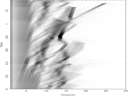
Figure 6: A trail diagram plotting values of $\eta(x)$ as a function of time as a greyscale. The broad lines in the plot indicate the path of optically thick shells – the breadth of the lines is the width of the profile function. Between $v=0\mbox{--}3.5$ the flow is smooth, instabilities grow exponentially in the range $v=3.5\mbox{--}6$, so that most of the gas is concentrated in the ballistically-moving shells at larger radii.

Figure 7: This plot of $\rho$ against $z$ is taken at $t=0.414$. The dense shells labelled with I, II, III match those whose histories are shown in the absorption trail plot, Fig.6.

4.2.2 Optically thin perturbation

(a)

(b)

Figure 8: Velocity (a) and density (b) plots for flow with an optically thin perturbation added. Data from two different times have been overlayed: $t=0.005$ (solid), $0.01$ (dashed). The prominent features of the plots are the advection of the optically thin perturbation in the upstream portion of the wind.

(a)

(b)

Figure 9: Velocity (a) and density (b) plots for the simulation shown in Fig. 9 at later times, $t=0.016$ (solid), $0.021$ (dashed). The advected material now becomes unstable and begins to break into dense shells.

A perturbation is applied to the base of the wind which is 10 grid elements thick ($\Delta z=0.0375$). The amplitude of the perturbation is a $v_{\rm p}=10\times v_{0}$ in velocity, and the change in density is $\rho_{\rm p}=\rho_{0}/10$, the subscript $0$ refers to background flow values; within this region, the velocity was increased to 10 times its previous value, and the density reduced by the same amount factor. These values were chosen to represent a typical short-wavelength ($1/k\ll\ell_{\rm Sob}$) perturbation, to compare with the analytical work from Owocki & Rybicki (1984), discussed above.

In this limit the evolution of the perturbation should follow equation (24). The gas in the perturbation experiences a constant acceleration, $\sim\tau_{0}\delta v$. In Fig. 8 the behaviour of the perturbation appears to be stable, as the gas in the perturbation is swept up into a dense shell which advects slowly across the grid. Behind this shell, the constant velocity gradient is characteristic of a free rarefaction.

Immediately ahead of the shell, the flow remains smoother than was the case in the unperturbed flow. It seems that the strong shock at the outer edge of the dense reduces the fetch available to the rapidly moving unstable outward radiative-acoustic waves, and so limits their amplitude in this region.

As the velocity gradient in the rarefaction decreases, instabilities form at the edges of the rarefaction, as can be seen in Fig. 9. Behind the dense shell, subsidiary shells form, while the smooth expansion of the gas upstream of the edge of the rarefaction also becomes highly disturbed. The optically thin subsidiary shells gather momentum from line driving and run up the diffuse wake of perturbation until they collide with the shock at the leading edge of the dense shell. This merging of shells is similar to that which occurs in the outer wind.

The dense shell is not subject to the formation of instabilities and is gently advected across the grid. This supports the asymptotic form, equation (23) which implies that this feature is stable for small wavelength perturbations: any change in the radiation force will only affect the phase of the perturbation, or the derivative of the velocity. The coupling of the radiation field with the dense shell is very weak which is evident in its unchanging amplitude, indicating that it is largely unaided by the driving force.

Shock structure begins to develop in the flow as an optically thin flow encounters a dense shell. A perfect example of a reverse shock can be seen in Fig. 10, a dense shell with a smoothly rarefied region preceding it. This figure also shows other shocks forming and interacting with the surrounding dense regions.

Figure 10: A plot of the flow at $t=0.028$, where reverse shock structure can be observed forming in the unstable wake of the initial perturbation (indicated by the arrow)

5 Numerical evolution of perturbations in two dimensions

The non-Sobolev approach described in the present paper can be naturally applied to multidimensional flows. In the present paper, we will concentrate on the simplest case, of the propagation of a single ray through plane-parallel flow. This is equivalent to studying a very narrow slice of the wind at a reasonable distance from the photosphere.

This has the obvious advantage that only a single ray calculation need be performed, parallel to one axis of the computational grid. It may be argued that this approach is little more than a series of one-dimensional simulations in separate but contiguous channels. However, while there is no tangential component to the radiation driving, we will see that the flows which are driven in this direction have a substantial effect on the structure of the wind.

The flows are studied in a similar way to the one-dimensional cases presented above. Perturbations are made to velocity field, added close to the base of the wind. A variety of widths and amplitudes of perturbation were modelled, but in the end the evolution of the flow always returns to structure of a similar form, so we will present here a small selection of typical results.

An initial two dimensional data set was obtained by filling each row of the simulation with identical data, derived from the unperturbed one dimensional run shown in Figure 3. Running the model without further perturbation, its development is similar initially to one-dimensional runs. However, as the simulation progresses these structures fragment in the tangential direction. It is to be presumed that these instabilities are seeded by small rounding errors in the underlying hydrodynamical scheme. Certainly the fragmentation initially appears nearly periodic.

The growth of these perturbations of the dense noise-excited shells may be attributed to Richtmeyer-Meshkov instability (a particular case of Rayleigh-Taylor instability which occurs when a shock interacts with a density discontinuity). As structure evolves from these instabilities, it has a very definite effect on the downstream flow. The result is a clumpy, highly structured flow as can be seen in Fig. 11.

If the gas is diffuse the instabilities do not evolve to macroscopic structure, because the strong coupling with the driving washes out the structure. Dense shells that have become optically thick, expand from gas pressure alone. This provides mechanisms by which both dense and diffuse shells can expand. Shocks are formed where the edges two such expanding shells collide, for example at (ii) in Fig. 12b. Depending on the expansion velocities of the shells involved, hydrodynamical instabilities may develop at the interface. The development of instabilities in the flow can fragment the resulting shell into multiply bullets and diffuse bubbles.

To study the development of these structures in more detail, we will now investigate the development of flows in which an explicit perturbation is included in the initial conditions.

Figure 11: The evolution of the flow when no perturbation is added . The structure develops as RM instabilities become a dominant feature in the flow. There is a complicated hydrodynamical interaction between shadowing, de-shadowing, and gas pressure expansion. The regular features result from the RM instabilities, however edge effects begin to arise as well as a high level of unresolved structure which disturbs the flow in an amorphous fashion. The axes measure the same distance code units as the one dimensional case. These and subsequent plots are scaled in the y-direction so that the complete set may be displayed together, for ease of comparison.

5.1 Velocity perturbed flow

Figure 12: The evolution of a velocity perturbation of 20 per cent above the background level is shown at variety of times, labelled beneath each plot. Many interesting features can be seen in this 2D model. As the perturbed gas moves through the background it appears to trigger Richtmeyer-Meshkov instabilities in the dense shells and causes a disturbance to the upstream background.

As a first example of the development of a perturbed two dimensional flow, we set the flow velocity to be $20$ per cent greater than its value at the equivalent depth in the surrounding flow in a region of $10\times 40$ grid elements (at a resolution of $1$ element $=0.00375$) at the base of the wind. Initially the disturbance expands smoothly through the background, and no significant effects appear on large scales. The matter in the initially perturbed region collects into a dense clump, with rarefied regions immediately upstream and downstream of it. The downstream rarefaction is simply the result of the increased velocity of the gas in the perturbed region, while the upstream perturbation is caused by the shadow of the perturbation. In this shadow, the gas experiences a decreased radiation force and so slows and is swept up by the clump.

As the perturbation increases in size, the changes of shadowing from gas shadowed by the perturbation (etc.) begin to have effects on the dense shells far downstream. The patch of the dense shell marked (i) in Fig. 12b, falls in the shadow of the perturbation, decelerates and becomes more diffuse, causing the first break in a shell structure. At this time an instability develops in the unshadowed parts of the dense shell where the optically thin faster flowing gas meets an optically thick slower dense shock. The disruption of the shells is dependent on whether they continue to contract as they evolve, which is in turn dependent on whether they are compressed by a shock behind or retarded by a dense region in ahead. If the shell expands slower than the perturbation evolves, the RM instability within the shell structure develops. If not the unstable structure diffuses away as the gas expands. This is the case in shell (ii) of Fig. 12c where the increasing radial width and decreasing density of the shell damps the instability, so that before it becomes significant the shell disperses. The shadowed region is unaffected by this expansion due to the alterations in spectrum that govern its motion. The apex of the shadowed region in the same plot forms a transient dense feature labelled (iii) which is created by the fast highly rarefied region immediately upstream of it, from which it accretes gas. As the flow evolves further, this clump disperses.

It is interesting to note that when part of a dense shell falls into the rarefied slipstream of the perturbation it experiences very little driving and is swept up by the dense clump of the perturbation. There is steady accretion from such incidents, increasing the density and extent of the perturbation. Were it not for this accretion the perturbation would become highly rarefied and disappear, but as is shown in Fig. 12d, part of the dense shell is accelerated and compressed into a high density bullet which rams through the perturbation.

Further downstream, Fig. 12e this feature develops into a bow shock/arrow shape and added to further by faster flowing gas accreting onto it from behind. This structure is preserved until the edge of the grid, but it is unlikely to remain in this form in the far downstream flow. When the wind has reached the terminal velocity adiabatic expansion will cause it to diffuse away.

Persistent features appear in the inner wind at the position of the initial perturbation. Instabilities seeded by these disrupt the formation of dense shells in the downstream flow. This is eventually smoothed out as the features spread in the tangential direction, Fig. 12f. However, as the flow is everywhere supersonic, the perturbations ought to have been advected downstream long before.

In an Eulerian hydrodynamical scheme, perturbations to smooth flow in a particular cell can only be removed exponentially with time (in essence by dilution). A sufficiently strong instability can decrease the exponential damping rate, or even force the perturbations to grow. This may be viewed as a limitation to the accuracy of these simulations – as indeed it would be a limitation to the accuracy of any Eulerian simulation with finite resolution (Lagrangian simulations would suffer from complementary problems as a result of sampling noise). However, in reality the flow will continually be affected by small scale perturbations from the photospheric flow. At late times, as the dense but noisy shells evolve they become highly structured as the hydrodynamics and the line-driving struggles for dominance in these regions. This flow is similar to that for unperturbed initial conditions, which suggests that it is not sensitive to the precise nature of the upstream perturbations, so long as they are small – the exponential growth of the instability erases the small details of its seeding.

5.2 Density perturbed flow

Figure 13: The evolution of a density perturbation of 20 per cent above the background level is shown at variety of times, labelled beneath each plot. These results contrast with those for a velocity perturbation shown earlier. Although the flow is similar the direction of the perturbation fronts is reversed.

Contrasting behaviour is observed if a density perturbation is applied to the background flow. The motivation for this choice of perturbation was interest in a macroscopic persistent feature in the outer portion of the wind. The phenomenon of Co-rotating Interaction Regions (CIRs) has been discussed previously (e.g. Dessart & Chesneau 2002) but as yet their formation is not well understood.

Initially, the perturbation expands in the form expected for such an overpressured region from pure hydrodynamics. A diffuse bubble appears, with dense shocked plates at its upstream and downstream edges. However, as the flow develops, these plates move apart and become more condensed, while the material between them is accelerated by line driving into the downstream clump, or is swept up by the approach of the upstream edge or clump. The direction which material will move and which clump it will be swept into is dependent on whether the gas falls in the shadow of the upstream clump or not.

The downstream flow still shows evidence of the spectral interference from the perturbation. The background dense shells are disturbed initially on the line of the edges of the perturbation, since at these positions a range of velocities are present while in the body of the perturbation has a very narrow velocity spread; the downstream material is only disturbed if gas upstream of it blocks radiation in a relevant frequency range.

The subsequent evolution of the upstream and downstream components of the original perturbation is distinct from that found in the previous section, showing sensitive dependence of the details of the flow on the initial conditions. One obvious feature, shown in Fig. 13b, is that both clumps of the perturbation appear to be blown away by the outflowing wind whereas in Fig. 12b the perturbation forms bow shocks as it pushes through slower material ahead of it.

These results prompted an investigation of a higher density initial perturbation, so a density perturbation by a factor of 4 times was applied to the same initial conditions as above. As one might expect the evolution of this perturbation, as seen in Fig. 14a-f is similar to that seen in Fig. 13a-f. In this case the upstream edge of the expanding bubble withstands disruption by the flow and eventually forms a ’v’-shaped front, which after further evolution develops highly detailed structure in Fig. 14d as a shock passes through it leaving RM instabilities to develop.

The structure from the downstream edge of the bubble forms features in Fig. 14c-d that are reminiscent of the structure in Fig. 13c-d. The perturbation has a great effect on the persistent features which remain in the upstream flow, leading to the beginning of highly clumped flow in Fig. 14f.

Figure 14: The evolution of a density perturbation a factor of 4 times the background level is shown at variety of times, labelled beneath each plot.

5.3 Physical consequences

Discrete Absorption Components [Kaper et al. 1999, DACs; e.g.] are significant features seen in the absorption profiles of unsaturated lines. Current observation suggests that the kinematics of these features is dominated by a rotational component, but theory has not addressed the manner in which they form and their dynamics as they move through the wind. The results of the above sections suggest that features that are formed in the early parts of the wind, are dispersed rapidly if their propagation is slow enough to be destroyed by RM instabilities. DACs are formed in the early part of a real wind when a slowly rotating region suffers a compression from a neighbouring fast moving region. Higher density compressed portions of the wind are observed in line spectra as DACs.

The dense, long lived bullets which are produced in our simulations are a strikingly similar to those inferred in some empirical models of DACs [Hamann et al. 2001, e.g.]. Similar structures would be expected to form as a result of variations in the stellar flux due to dark surface features, which may naturally explain the origin of CIRs.

The ultimate aim of these models is to understand the nature of observed hot star winds. While the present results are by no means definitive, it is clear that cohesive absorbing knots are a natural feature of line-driven winds. However, further, more physically detailed, numerical simulations will be required before a detailed comparison to the observations of wind structures such as DACs can be performed.

6 Summary

We present models of the structure of unstable line-driven flows, calculated in two dimensions with a full hydrodynamical code and non-local radiation transport.

Our results compare well to those of more physically complete (but geometrically restricted) models in their common limits. The reproduction of the noise waves and the dominance of reverse shocks in the downstream structure is in good agreement with those seen by other non-Sobolev approaches (e.g. OCR, Runacres & Owocki 2002, Feldmeier 1995). This behaviour is borne out by the close similarity of the statistical descriptors of the flows we study to the results presented by Runacres & Owocki (2002). This suggests that the current model does indeed present a good description of the non-Sobolev behaviour of this wind.

The model presented here has limitations: 1) the gas is taken to be isothermal, which is reasonable at least in high density regions; 2) the spatial domain is restricted, effectively to a small region reasonably far from the photosphere; 3) the line profile function is taken to have a top-hat form rather than a Gaussian or Voigt profile; 4) the fiducial value of $v_{\rm th}/c_{\rm s}=0.5$ was used [Owocki 1991, following], although a rather lower value may in fact be more appropriate; 5) we have treated the radiation transfer in the pure-absorption approximation. We have argued, however, that none of these approximations will have a significant effect on the local structure of the line-driven winds, which is our principal interest in this paper: our work complements other studies in which these processes are treated in more physical detail in a more geometrically restricted domain.

In future work, we will include the line-drag effect of scattered radiation [Lucy 1984] [Owocki & Puls 1996, formulated in the non-Sobolev method by]. The asymmetry we have shown between forward and backward calculation of the Sobolev line force from the wind velocity gradient, could be of use in approximating the fore/aft asymmetry which produces line drag. Since this is a local effect, it may not be necessary to use a full non-Sobolev method for its calculation. Indeed a Sobolev approach may actually be more suitable than a global method for simulations with high degrees of imposed symmetry.

References

- [Abbott 1980] Abbott D., 1980, ApJ, 242, 1183
- [Babel 1996] Babel J., 1996, A&A, 309, 867
- [Carlberg 1980] Carlberg R. G., 1980, ApJ, 241, 1131
- [Castor et al. 1975] Castor J. I., Abbott D. C., Klein R. I., 1975, ApJ, 195, 157 (CAK)
- [Collela & Woodward 1984] Colella P., Woodward P. R., 1984, JCP, 54, 174
- [Dessart & Chesneau 2002] Dessart L., Chesneau O., 2002, A&A, 383, 1113
- [Feldmeier 1995] Feldmeier A., 1995, A&A, 299, 523
- [Gayley et al. 2001] Gayley K. G., Ignace R., Owocki S. P., 2001, ApJ, 558, 802
- [Hamann et al. 2001] Hamann, W.-R., Brown, J. C., Feldmeier, A., Oskinova, L. M., 2001 A&A,378,946
- [Kaper et al. 1999] Kaper, L., Henrichs, H. F., Nichols, J. S., Telting, J. H., 1999A&A, 344, 231
- [Lamers & Morton 1976] Lamers H. J. G. L. M., Morton D. C., ApJ Sup, 32, 715
- [Lucy 1984] Lucy L. B., 1984, ApJ, 284, 351
- [Lucy & Soloman 1970] Lucy L. B., Solomon P., ‘970, ApJ, 159, 879
- [Owocki 1991] Owocki S. P., 1991, in van der Hucht K. A., Hidayat, B., eds, IAU Symp. 147, Wolf-Rayet stars and interrelations with other massive stars, p. 155
- [Owocki 1999] Owocki S. P., 1999, in Wolf, B., Stahl, O.,and Fullerton, A. W., eds, IAU Colloquium 169, Variable and Non-spherical Stellar Winds in Luminous Hot Stars
- [Owocki et al. 1988] Owocki S. P., Castor, J. I., Rybicki G. B., 1988, ApJ, 335, 914 (OCR)
- [Owocki & Puls 1996] Owocki S. P., Puls J., 1996, ApJ, 462, 894
- [Owocki & Rybicki 1984] Owocki S. P., Rybicki, G. B. 1984, ApJ, 284, 337
- [Poe et al. 1990] Poe C. H., Owocki S. P., Castor J. I., 1990, ApJ, 358, 199
- [Proga et al. 1998] Proga D., Stone J. M., Drew J. E., 1998, MNRAS, 295, 595
- [Runacres & Owocki 2002] Runacres M. C., Owocki S. P., 2002, A&A, 381, 1015
- [Sobolev 1960] Sobolev V. V., 1960, Moving Envelopes of Stars, Havard Univ. Press, Cambridge, MA
- [Wang et al. 2000] Wang L. J., Kuzmich A., Dogariu A., 2000, Nature, 406, 277