The Effects of the Tidal Force on Shear Instabilities in the Dust Layer of the Solar Nebula

Abstract

The linear analysis of the instability due to vertical shear in the dust layer of the solar nebula is performed. The following assumptions are adopted throughout this paper: (1) The self-gravity of the dust layer is neglected. (2) One fluid model is adopted, where the dust aggregates have the same velocity with the gas due to strong coupling by the drag force. (3) The gas is incompressible.

The calculations with both the Coriolis and the tidal forces show that the tidal force has a stabilizing effect. The tidal force causes the radial shear in the disk. This radial shear changes the wave number of the mode which is at first unstable, and the mode is eventually stabilized. Thus the behavior of the mode is divided into two stages: (1) the first growth of the unstable mode which is similar to the results without the tidal force, and (2) the subsequent stabilization due to an increase of the wave number by the radial shear. If the midplane dust/gas density ratio is smaller than 2, the stabilization occurs before the unstable mode grows largely. On the other hand, the mode grows faster by one hundred orders of magnitude, if this ratio is larger than 20.

Because the critical density of the gravitational instability is a few hundreds times as large as the gas density, the hydrodynamic instability investigated in this paper grows largely before the onset of the gravitational instability. It is expected that the hydrodynamic instability develops turbulence in the dust layer and the dust aggregates are stirred up to prevent from settling further. The formation of planetesimals through the gravitational instabilities is difficult to occur as long as the dust/gas surface density ratio is equal to that for the solar abundance.

On the other hand, the shear instability is suppressed and the planetesimal formation through the gravitational instability may occur, if dust/gas surface density ratio is hundreds times as large as that for the solar abundance.

Key Words: Planetary Formation; Solar Nebula,

I. INTRODUCTION

Planetesimal formation in the solar nebula is one of unresolved issues in the theory of planetary formation. In the solar nebula, micron-sized dust particles which float uniformly at first are considered to stick each other by non-gravitational forces (e.g., the van der Waals force) to form dust aggregates. If the solar nebula is laminar, the dust aggregates settle toward the midplane, and simultaneously they stick each other by collisions due to differential settling velocities. Thus, a thin dust layer is formed around the midplane. The dust density around the midplane increases gradually due to the dust settling. When the dust self-gravity exceeds the tidal force of the central star, that is, the density exceeds the critical density $\rho_{c}$, the dust layer becomes gravitationally unstable and fragments into a lot of km-sized planetesimals (Safronov 1969, Goldreich and Ward 1973, Coradini et al. 1981, Sekiya 1983). Formerly the above mentioned gravitational instability model was considered to be the most promising process of planetesimal formation.

However, if the solar nebula is turbulent, dust aggregates are stirred up, and it may be difficult for the dust density to exceed the critical density of the gravitational instability. Several causes of turbulence in the solar nebula have been proposed: the thermal convection (Lin and Papaloizou 1980, Cabot et al. 1987a, b, Ruden et al. 1988), the hydrodynamic instability due to radial shear in the disk (Papaloizou and Pringle 1984, Goldreich and Narayan 1985, Narayan et al. 1987, Nakagawa and Sekiya 1992, Sekiya et al. 1993), and the magneto-rotational instability (Balbus and Hawley 1991), and so on. This work concentrates on investigating the instability due to vertical shear in the dust layer, which arises by the dust settling itself as explained in the following. If the drag force did not work, dust aggregates would revolve with the Kepler velocity balancing the centrifugal force and the gravitational force of a central star. On the other hand, a gas fluid would revolve slightly slower than the Kepler velocity because only gas is partially supported by a gas pressure gradient. Thus, when gas and dust drag each other, their velocities depend on the dust to gas mass ratio and the frictional time. In particular, when the frictional time is much shorter than a Kepler period, namely that dust aggregate is small and/or fluffy, a dust aggregate and gas fluid move approximately with a same velocity. Then, the revolution velocity $\bar{v}$ in the co-ordinate system which moves with the local Kepler velocity $v_{K}$ is given by

$$\bar{v}=-\frac{\rho_{g}}{\rho}\eta v_{K}.$$ (1)

Here $\rho$ is the total fluid density defined by

$$\rho=\rho_{g}+\rho_{d},$$ (2)

where $\rho_{g}$ is the gas density and $\rho_{d}$ is the dust density. The non-dimensional parameter $\eta$ represents the effect of the radial pressure gradient:

$$\eta=-\frac{r}{2\rho_{g}v_{K}^{2}}\frac{\partial P}{\partial r},$$ (3)

where $r$ is the distance from the rotation axis of the disk and $P$ is the gas pressure (Adachi et al. 1976, Weidenschilling 1977, Nakagawa et al. 1986, Sekiya 1998). This vertical shear may cause the shear instability, which may develop turbulence in the dust layer; thus dust aggregates may be stirred up and dust density may not exceed the critical density of the gravitational instability (Weidenschilling 1980).

Cuzzi et al. (1993) have performed numerical simulations of two fluids, gas and dust, in order to examine whether the above mentioned turbulence is strong enough to prevent the gravitational instability of the dust layer. They assumed single-sized compact aggregates (10cm or 60cm). They obtained the quasi-equilibrium density distributions balancing the turbulent diffusion and the settling of aggregates. They showed that the density does not reach the critical density of the gravitational instability. Champney et al. (1995) extended this model to multi-fluids where different sized dust aggregates existed in the gas. Dobrovolskis et al. (1999) made calculations including the dissipation due to the friction between dust aggregates and the gas. The results of these papers are almost same as Cuzzi et al. (1993). The parameters used in the turbulence model of these papers were estimated from the laboratory experiments without the density stratification and the effects of the Coriolis and the tidal forces.

Sekiya (1998) obtained the quasi-equilibrium distributions of dust density, including the effect of the density stratification, but neglecting the effects of the Coriolis and the tidal forces. The vertical shear rate $\partial v/\partial z$ increases as dust aggregates settle toward the midplane, where $z$ is the distance from the midplane. Eventually, the shear rate exceeds the critical value of the shear instability, i.e., the Richardson number becomes less than 0.25. The Richardson number is defined by

$$J=-\frac{g_{z}\partial\rho/\partial z}{\rho(\partial\bar{v}/\partial z)^{2}},$$ (4)

where $g_{z}$ is the vertical gravitational acceleration. Then turbulence may be developed. If dust aggregates are small enough, very weak turbulence can stir up the dust aggregates and prevent them from settling further. Thus, the dust density distribution regulates itself so that the shear rate is marginally above the critical value $J_{c}=0.25$. Sekiya (1998) calculated analytically this density distribution with the critical shear rate. He has concluded that the dust density hardly exceeds the critical density of the gravitational instability, as long as the dust to gas mass ratio inferred from the solar abundance is assumed. He has shown that if the dust to gas mass ratio increases one order of magnitude by gas escape or dust concentration, the dust density at the midplane exceeds the critical value of the shear instability, and planetesimal can be formed through gravitational fragmentation of the dust layer.

Youdin and Shu (2002) also found the critical ratio of the surface density ratio of dust and gas using the density distribution with the critical shear rate. In addition, they suggested a dust concentration mechanism through radial drift of chondrule-sized dust by gas drag in the nebula. This mechanism enables the density ratio of dust and gas to exceed the critical value in $\leq$ few $\times 10^{6}$ year.

The derivation of dust density distribution by Sekiya (1998), and Youdin and Shu (2002) was somewhat intuitive. More elaborate calculations of the shear instability are needed in order to conclude that the gravitational instability model of planetesimal formation is denied. For the first step, Sekiya and Ishitsu (2000, 2001) (Hereafter Papers I and II) investigated the shear instability of the dust layer using the linear analysis, neglecting the effects of the Coriolis and the tidal forces.

In Paper I, we assumed that the unperturbed density had the constant Richardson number density distributions by Sekiya (1998). The results show: (A) The flow is stable for the Richardson number $J\mathrel{\hbox to0.0pt{\raise 2.20013pt\hbox{$>$}\hss}{\lower 2.20013pt\hbox{$\sim$}}}0.22$. (B) The growth time of the shear instability is much longer than the Kepler period, as long as the Richardson number $J\mathrel{\hbox to0.0pt{\raise 2.20013pt\hbox{$>$}\hss}{\lower 2.20013pt\hbox{$\sim$}}}0.1$. On the other hand, the Coriolis and the tidal forces would affect the flow in time scale on the order of the Kepler period. Thus the neglect of these forces is not good for the constant Richardson number density distribution with $J\mathrel{\hbox to0.0pt{\raise 2.20013pt\hbox{$>$}\hss}{\lower 2.20013pt\hbox{$\sim$}}}0.1$.

In Paper II, the linear stability analysis was performed using the following density distribution which will be called the hybrid density distribution (an inner constant density distribution, plus outer sinusoidal transition regions):

$$\rho_{d0}(z)=\left\{\begin{array}[]{rl}\rho_{d0}(0)&\mbox{for $|z|\leq z_{d}-2h_{d}$,}\\ \rho_{d0}(0)\{1-\sin[\pi(z-z_{d}+h_{d})/2h_{d}]\}/2&\mbox{for $z_{d}-2h_{d}<|z|<z_{d}$,}\\ 0&\mbox{for $z_{d}\leq|z|$},\end{array}\right.$$ (5)

where $z_{d}$ the half-thickness of the dust layer, and $h_{d}$ the half-thickness of the transition zones, where the dust density varies from $\rho_{d0}(0)$ to 0 sinusoidally. Here the half-thickness of the dust layer is given by

$$z_{d}=\frac{\Sigma_{d}}{2\rho_{d0}(0)}+h_{d},$$ (6)

and the surface density of the dust is given by

$$\Sigma_{d}=\int_{-\infty}^{+\infty}\rho_{d}dz=\left\{\begin{array}[]{rl}7.1f_{d}(r/\mbox{AU})^{-1.5}\mbox{g cm}^{2}\mbox{ for }r<2.8\mbox{AU},\\ 30f_{d}(r/\mbox{AU})^{-1.5}\mbox{g cm}^{2}\mbox{ for }r>2.8\mbox{AU},\end{array}\right.$$ (7)

where $\rho_{d}$ is the dust density defined by the total dust mass floating in a unit volume, and $f_{d}$ is a parameter ($f_{d}=1$ for the Hayashi model). We used Hayashi’s solar nebula model (Hayashi 1981, Hayashi et al., 1985) at 1AU as the dust surface density $\Sigma_{d}$ in the most of calculations except for Figs. 4, 20, and 21.

In the following, we explain the reason why the hybrid density distribution is used. Dust particles which are distributed uniformly at first stick together to form dust aggregates. In a laminar nebula, the settling velocity $v_{dz}$ of a dust aggregate is given by

$$v_{dz}=-\tau_{f}\Omega_{K}^{2}z,$$ (8)

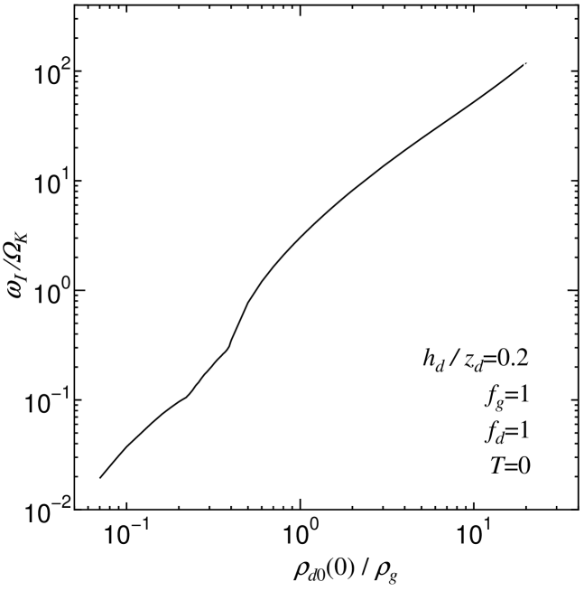
Figure 2: The growth rate $\omega_{I}$ of the mode with the most unstable wave number as a function of the ratio of dust to gas on the midplane $\rho_{d0}(0)/\rho_{g}$, in the case where $T=0$ with $h_{d}/z_{d}=0.2$.

where $\tau_{f}$ is the frictional time of the dust aggregate. Dust aggregates grow faster in regions with larger $|z|$, since the principal relative velocity of dust aggregates is induced by difference of settling velocities of dust aggregates with different frictional times (Weidenschilling 1980, Nakagawa et al. 1981). As dust aggregates grow, their settling velocities increase if the dust aggregates are compact. Thus, dust aggregates accumulate in a certain region with an intermediate value of $|z|$ (see 1000 yrs and 1300 yrs density distribution in Fig. 2 of Nakagawa et al. (1981)). This state is unstable for the Rayleigh-Taylor instability, and the dust density distribution is considered to be adjusted as to be constant in the dust layer (Watanabe and Yamada 2000). Thus, the constant distribution in the dust layer as given by Eq. (5) for $|z|\leq z_{d}-2h_{d}$ is considered to be a natural consequence of the dust settling in a laminar disk. For simplicity, the sinusoidal density distribution is assumed in the transition region ($z_{d}-2h_{d}<|z|<z_{d}$).

According to results of Paper II, if $\rho_{d}(0)/\rho_{g}\sim 1$, the growth rate of the instability is on the order of the Keplerian angular frequency. On the other hand, if $\rho_{d}(0)/\rho_{g}>>1$, the growth rate is much larger than the Keplerian angular frequency. Thus, we have expected that the Coriolis and tidal forces might not have an important effect as long as $\rho_{d}(0)/\rho_{g}>>1$.

Ishitsu and Sekiya (2002) (Hereafter Paper III), carried out calculations taking the Coriolis force into account, but neglecting the tidal force. The results showed that the Coriolis force had little effects. However, we found a new type of resonances which resembles the Lindbland resonances if the growth rate is similar to or smaller than the Keplerian angular frequency. The energy source of the instability is this resonance and different from that of the shear instability. These results will be reviewed in Section 4.

In this paper, we solve linearized perturbation equations with the tidal and the Coriolis forces under the following assumptions: (1) The self-gravity is neglected. (2) A mixture of gas and dust is treated as one fluid, which is a good approximation in the case where dust aggregate sizes are small ($\mathrel{\hbox to0.0pt{\raise 2.20013pt\hbox{$<$}\hss}{\lower 2.20013pt\hbox{$\sim$}}}$ 1cm). (3) The gas is incompressible since the dust layer which is much less than vertical scale height of the gas disk $H$ is treated. (4) The effects of the radial density and the pressure gradient of the unperturbed state are only incorporated in the unperturbed rotation velocity distribution $v_{0}(z)$. (5) Local Cartesian coordinates ($x,y,z$) are used and we neglect the curvature of a circle with constant values of $r$ and $z$. (6) The hybrid dust density distribution used in Papers II and III is adopted as the unperturbed dust density distribution.

When the dust layer with the hybrid dust density distribution becomes unstable for a linear perturbation, the linear mode grows. Eventually, nonlinear effects become important, and a quasi-equilibrium state between settling and turbulent diffusion of dust aggregates would be realized. This paper treats the first linear growth of the instability. Of course, it is very important to obtain quasi-equilibrium state with taking account of the Coriolis and the tidal forces, which is left in future works. Note that $J=$const distribution obtained Sekiya (1998) is not necessarily realize, since it neglects the effects of the Coriolis and the tidal forces.

In Section II, the basic equations for the linear analysis are derived. In Section III, a numerical method is described. In Section IV, solutions with the Coriolis force but without the tidal force (Paper III) are reviewed. In Section V, solutions with both the Coriolis and the tidal forces are given. In Section VI, conclusions obtained in this paper are summarized.

II. FORMULATION

We use the local Cartesian coordinate system around a radius $R$ from the central star rotating with the Kepler angular frequency $\Omega_{K}(R)$:

$$x=r-R,$$ (9)

$$y=R[\phi-\Omega_{K}(R)t],$$ (10)

$$z=z,$$ (11)

where the curvature of $r=$ constant circle is neglected since $O(\partial/\partial r)>>O(1/r)$ and $(\partial/\partial{\phi})/r\approx(\partial/\partial y)$ for $r>>|x|,|y|$.

In the rotational system that revolves around a central star with angular frequency $\Omega_{K}(R)$, the Coriolis and the centrifugal forces emerge. The tidal force, resultant force of gravity of central star and centrifugal force, is given in the local approximation regime by $3x\Omega_{K}^{2}(R)$. Hereafter, $\Omega_{K}(R)$ is denoted by $\Omega_{K}$ for simplicity. Note that $\Omega_{K}$ is constant. The hydrodynamic equations are given for the local Cartesian co-ordinates which move azimuthally with the Kepler velocity $v_{K}$ and rotate with the Kepler angular velocity $\Omega_{K}$ by

$$\frac{\partial u}{\partial x}+\frac{\partial v}{\partial y}+\frac{\partial w}{\partial z}=0,$$ (12)

$$\frac{\partial\rho}{\partial t}+u\frac{\partial\rho}{\partial x}+v\frac{\partial\rho}{\partial y}+w\frac{\partial\rho}{\partial z}=0,$$ (13)

$$\frac{\partial u}{\partial t}+u\frac{\partial u}{\partial x}+v\frac{\partial u}{\partial y}+w\frac{\partial u}{\partial z}=-\frac{1}{\rho}\frac{\partial P}{\partial x}+3T\Omega_{K}^{2}x+2\Omega_{K}v.$$ (14)

$$\frac{\partial v}{\partial t}+u\frac{\partial v}{\partial x}+v\frac{\partial v}{\partial y}+w\frac{\partial v}{\partial z}=-\frac{1}{\rho}\frac{\partial P}{\partial y}-2\Omega_{K}u,$$ (15)

$$\frac{\partial w}{\partial t}+u\frac{\partial w}{\partial x}+v\frac{\partial w}{\partial y}+w\frac{\partial w}{\partial z}=-\frac{1}{\rho}\frac{\partial P}{\partial z}-\Omega_{K}^{2}z,$$ (16)

Note that only the case $T=1$ is realistic; on the other hand, the case $T=0$ corresponds to the model used in Paper III, where the tidal force is neglected. In this paper, calculations are performed for $0\leq T\leq 1$, in order to elucidate the effect of the tidal force on the instability in the dust layer. If $u=P=0$, Eq. (14) reads

$$v=-\frac{3}{2}T\Omega_{K}x.$$ (17)

This expresses the circular Kepler motion in the local coordinate system (for $T=1$). In order to eliminate the Keplerian part of the velocity, we introduce the velocity relative to the Keplerian motion.

$$\bar{v}=v+\frac{3}{2}T\Omega_{K}x.$$ (18)

From Eqs. (12) to (16), we have

$$\frac{\partial u}{\partial x}+\frac{\partial\bar{v}}{\partial y}+\frac{\partial w}{\partial z}=0,$$ (19)

$$\frac{\partial\rho}{\partial t}+u\frac{\partial\rho}{\partial x}+(\bar{v}-\frac{3}{2}T\Omega_{K}x)\frac{\partial\rho}{\partial y}+w\frac{\partial\rho}{\partial z}=0,$$ (20)

$$\frac{\partial u}{\partial t}+u\frac{\partial u}{\partial x}+(\bar{v}-\frac{3}{2}T\Omega_{K}x)\frac{\partial u}{\partial y}+w\frac{\partial u}{\partial z}=-\frac{1}{\rho}\frac{\partial P}{\partial x}+2\Omega_{K}\bar{v},$$ (21)

$$\frac{\partial\bar{v}}{\partial t}+u\frac{\partial\bar{v}}{\partial x}+(\bar{v}-\frac{3}{2}T\Omega_{K}x)\frac{\partial\bar{v}}{\partial y}+w\frac{\partial\bar{v}}{\partial z}=-\frac{1}{\rho}\frac{\partial P}{\partial y}-(2-\frac{3}{2}T)\Omega_{K}u,$$ (22)

$$\frac{\partial w}{\partial t}+u\frac{\partial w}{\partial x}+(\bar{v}-\frac{3}{2}T\Omega_{K}x)\frac{\partial w}{\partial y}+w\frac{\partial w}{\partial z}=-\frac{1}{\rho}\frac{\partial P}{\partial z}-\Omega_{K}^{2}z.$$ (23)

In order to carry out linear calculations, we assume that an unperturbed state is steady and uniform in $x$ and $y$ directions:

$$\frac{\partial}{\partial t}=\frac{\partial}{\partial x}=\frac{\partial}{\partial y}=0.$$ (24)

We also assume that the unperturbed velocity is parallel to $y$-axis (i.e. azimuthal direction)

$$u_{0}=w_{0}=0.$$ (25)

From Eqs. (21), (23) and (25), we have

$$\frac{1}{\rho_{0}}\frac{\partial P_{0}}{\partial x}=2\Omega_{K}{\bar{v}_{0}},$$ (26)

and

$$\frac{1}{\rho_{0}}\frac{\partial P_{0}}{\partial z}=-\Omega_{K}^{2}z,$$ (27)

respectively.

The unperturbed azimuthal velocity is calculated from a given dust density distribution $\rho_{d0}$ and a given value of $\eta$ by using Eqs. (1) and (2):

$$\bar{v}_{0}=-\frac{\rho_{g}}{\rho_{0}}\eta v_{K},$$ (28)

where values of $\rho_{g}$, $\eta$, $v_{K}$ are assumed to be constant, and $\rho_{0}$ depends only on $z$ and is independent of $x$ in the local approximation with $r\approx R$. The midplane gas density $\rho_{g}=\rho_{g}(0)$ is given by

$$\rho_{g}(0)=\sqrt{\pi}\Sigma_{g}/H,$$ (29)

where $\Sigma_{g}$ is surface gas density:

$$\Sigma_{g}=1700f_{g}(r/\mbox{AU})^{-1.5}\mbox{g cm}^{2},$$ (30)

and $f_{g}$ is a parameter ($f_{g}=1$ for the Hayashi model). The radial pressure gradient $\partial P_{0}/\partial x$ is then given by Eq. (26).

Linearizing Eqs. (19) to (23) and using Eqs. (26) and (27), we have

$$\frac{\partial u_{1}}{\partial x}+\frac{\partial v_{1}}{\partial y}+\frac{\partial w_{1}}{\partial z}=0,$$ (31)

$$\frac{\partial\rho_{1}}{\partial t}+(\bar{v}_{0}-\frac{3}{2}T\Omega_{K}x)\frac{\partial\rho_{1}}{\partial y}+\frac{d\rho_{0}}{dz}w_{1}=0,$$ (32)

$$\frac{\partial u_{1}}{\partial t}+(\bar{v}_{0}-\frac{3}{2}T\Omega_{K}x)\frac{\partial u_{1}}{\partial y}=-\frac{1}{\rho_{0}}\frac{\partial P_{1}}{\partial x}+2\Omega_{K}\frac{\bar{v}_{0}}{\rho_{0}}\rho_{1}+2\Omega_{K}v_{1},$$ (33)

$$\frac{\partial v_{1}}{\partial t}+(\bar{v}_{0}-\frac{3}{2}T\Omega_{K}x)\frac{\partial v_{1}}{\partial y}+\frac{dv_{0}}{dz}w_{1}=-\frac{1}{\rho_{0}}\frac{\partial P_{1}}{\partial y}-(2-\frac{3}{2}T)\Omega_{K}u_{1}$$ (34)

$$\frac{\partial w_{1}}{\partial t}+(\bar{v}_{0}-\frac{3}{2}T\Omega_{K}x)\frac{\partial w_{1}}{\partial y}=-\frac{1}{\rho_{0}}\frac{\partial P_{1}}{\partial z}-\frac{\Omega_{K}^{2}z}{\rho_{0}}\rho_{1}.$$ (35)

The normal mode analysis (i.e. the Fourier transform) for $x$ cannot be done in this coordinates system because the coefficients of equations depend on $x$. Thus we transform coordinate $y$ into the shearing coordinate $y^{\prime}$ with velocity $-\frac{3}{2}T\Omega_{K}x$ in order that the normal mode analysis for $x$ can be done (see e.g., Goldreich and Lynden-Bell 1965, Goldreich and Tremaine 1978, Ryu and Goodman 1992):

$$y^{\prime}=y+\frac{3}{2}T\Omega_{K}xt.$$ (36)

We assume that perturbed quantities are written

$$f_{1}(x,y,z,t)=\hat{f}_{1}(z,t)\exp[i(k_{y}y^{\prime}+k_{x}x)].$$ (37)

Substituting this expression into Eqs. (31)–(35), the perturbation equations are rewritten

$$ik^{\prime}_{x}u_{1}+ik_{y}v_{1}+\frac{\partial w_{1}}{\partial z}=0,$$ (38)

$$\frac{\partial\rho_{1}}{\partial t}+ik_{y}\bar{v}_{0}\rho_{1}+\frac{d\rho_{0}}{dz}w_{1}=0,$$ (39)

$$\frac{\partial u_{1}}{\partial t}+ik_{y}\bar{v}_{0}u_{1}=-ik^{\prime}_{x}\frac{1}{\rho_{0}}P_{1}+2\Omega_{K}\frac{\bar{v}_{0}}{\rho_{0}}\rho_{1}+2\Omega_{K}v_{1},$$ (40)

$$\frac{\partial v_{1}}{\partial t}+ik_{y}\bar{v}_{0}v_{1}=-ik_{y}\frac{1}{\rho_{0}}P_{1}-\frac{d\bar{v}_{0}}{dz}w_{1}-\left(2-\frac{3}{2}T\right)\Omega_{K}u_{1}$$ (41)

$$\frac{\partial w_{1}}{\partial t}+ik_{y}\bar{v}_{0}w_{1}=-\frac{1}{\rho_{0}}\frac{\partial P_{1}}{\partial z}-\frac{\Omega_{K}^{2}z}{\rho_{0}}\rho_{1},$$ (42)

where,

$$k^{\prime}_{x}=k_{x}+\frac{3}{2}Tk_{y}\Omega_{K}t.$$ (43)

Here, we cannot use the Fourier transform method with respect to t because the coefficients of these equations depend on $t$. The linearized equations must be integrated numerically by using the finite difference method in order to see the growth of an instability.

Boundary conditions for $z$-direction are given as follows. Only odd solutions for $w_{1}$ (i.e. $w_{1}=0$ at $z=0$) are considered since even ones are always stable according to our calculations. The continuity of pressure at the boundary between the dust and gas layers were applied in the analytical method of Papers I to III, but it is difficult to apply this condition to our numerical method. Thus, we solve the perturbation equation numerically within region $[0,z_{0}]$ where the solid-wall condition is applied at the boundary for simplicity. The value of $z_{0}$ should be large enough in order for an eigenfunction to decay sufficiently at a boundary $z_{0}$. It was confirmed that numerical solutions for $T=0$ with this condition agree well with solutions of the Paper III. Thus, the boundary conditions are given by

$$w_{1}=0\;\mbox{ at }\;z=0\mbox{ and }z_{0}.$$ (44)

From Eqs. (42) and (44), we have

$$\frac{\partial P_{1}}{\partial z}+\Omega_{K}^{2}z\rho_{1}=0\;\mbox{ at }\;z=0\mbox{ and }z_{0}.$$ (45)

From Eqs. (39) and (44), we have

$$\frac{\partial\rho_{1}}{\partial t}+ik_{y}\bar{v}_{0}\rho_{1}=0\;\mbox{ at }\;z=0\mbox{ and }z_{0}.$$ (46)

If we give an initial condition with $\rho_{1}=0$ at $z=0\mbox{ and }z_{0}$, Eq. (46) implies that $\rho_{1}=0$ for $t\geq 0$. Hereafter we take only such initial conditions for simplicity. Accordingly boundary conditions for $P_{1}$ and $\rho_{1}$ are given by

$$\frac{\partial P_{1}}{\partial z}=0\;\mbox{ at }\;z=0\mbox{ and }z_{0},$$ (47)

$$\rho_{1}=0\;\mbox{ at }\;z=0\mbox{ and }z_{0}.$$ (48)

III. NUMERICAL METHOD

We adopt MAC method (Harlow and Welch 1965), i.e. pressure is determined by the condition that the equation of continuity is satisfied in the next step, and other variables $u_{1},v_{1},w_{1}$ and $\rho_{1}$ are calculated using this value of pressure.

We define the divergence of a perturbed velocity by

$$D\equiv ik^{\prime}_{x}u_{1}+ik_{y}v_{1}+\frac{\partial w_{1}}{\partial z}.$$ (49)

Multiplying Eq. (40) by $ik^{\prime}_{x}$ and Eq. (41) by $ik_{y}$, and taking partial derivative Eq. (42) with respect to $z$, and adding, we have

$$\frac{\partial D}{\partial t} = -ik_{y}\bar{v}_{0}D-2ik_{y}\frac{d\bar{v}_{0}}{dz}w_{1}-\frac{1}{\rho_{0}}\left(-k^{\prime 2}_{x}-k^{2}_{y}+\frac{\partial^{2}}{\partial z{}^{2}}\right)P_{1}+\frac{1}{\rho_{0}^{2}}\frac{d\rho_{0}}{dz}\frac{\partial P_{1}}{\partial z}$$ (50)

$$+2i\Omega_{K}k^{\prime}_{x}\frac{\bar{v}_{0}}{\rho_{0}}\rho_{1}+2i\Omega_{K}k^{\prime}_{x}v_{1}-i\left(2-3T\right)\Omega_{K}k_{y}u_{1}+\Omega_{K}^{2}\frac{d}{dz}\left(-\frac{z}{\rho_{0}}\rho_{1}\right).$$

We use the first order approximation:

$$\frac{\partial D}{\partial t}\approx\frac{D^{n+1}-D^{n}}{\Delta t}.$$ (51)

We require that the equation of continuity (38) is satisfied in the next step, i.e. $D^{n+1}=0$. Thus, we get the Poisson equation for $P_{1}$:

$$\left(-k^{\prime n2}_{x}-k^{2}_{y}+\frac{\partial^{2}}{\partial z{}^{2}}-\frac{1}{\rho_{0}}\frac{d\rho_{0}}{dz}\frac{\partial}{\partial z}\right)P_{1}^{n}$$ (52)

$$= \rho_{0}\left\{\left(\frac{1}{\Delta t}-2ik_{y}\bar{v}_{0}\right)D^{n}-2ik_{y}\frac{d\bar{v}_{0}}{dz}w_{1}^{n}+2i\Omega_{K}k^{\prime n}_{x}v_{1}^{n}-i\left(2-3T\right)\Omega_{K}k_{y}u_{1}^{n}\right.$$

$$\left.+2i\Omega_{K}k^{\prime n}_{x}\frac{\bar{v}_{0}}{\rho_{0}}\rho_{1}^{n}+\Omega_{K}^{2}\frac{d}{dz}\left(-\frac{z}{\rho_{0}}\rho_{1}^{n}\right)\right\}.$$

From this equation, we can get $P_{1}$ at the time step $n$. Next, we calculate $\rho_{1},u_{1},v_{1}$ and $w_{1}$ at the time step $n+1$ from Eqs. (39)–(42):

$$\rho_{1}^{n+1}=\rho_{1}^{n}+\Delta t\left\{-ik_{y}\bar{v}_{0}\rho_{1}^{n}-\frac{d\rho_{0}}{dz}w_{1}^{n}\right\},$$ (53)

$$u_{1}^{n+1}=u_{1}^{n}+\Delta t\left\{-ik_{y}\bar{v}_{0}u_{1}^{n}-ik^{\prime n}_{x}\frac{1}{\rho_{0}}P_{1}^{n}+2\Omega_{K}\frac{\bar{v}_{0}}{\rho_{0}}\rho_{1}^{n}+2\Omega_{K}v_{1}^{n}\right\},$$ (54)

$$v_{1}^{n+1}=v_{1}^{n}+\Delta t\left\{-ik_{y}\bar{v}_{0}v_{1}^{n}-\frac{d\bar{v}_{0}}{dz}w_{1}^{n}-ik_{y}\frac{1}{\rho_{0}}P_{1}^{n}-\left(2-\frac{3}{2}T\right)\Omega_{K}u_{1}^{n}\right\},$$ (55)

$$w_{1}^{n+1}=w_{1}^{n}+\Delta t\left\{-ik_{y}\bar{v}_{0}w_{1}^{n}-\frac{1}{\rho_{0}}\frac{\partial P_{1}^{n}}{\partial z}-\frac{\Omega_{K}^{2}z}{\rho_{0}}\rho_{1}^{n}\right\}.$$ (56)

The above method is the first order accuracy with respect to $\Delta t$. In order to improve them to the second order accuracy, we use the following strategy. We replace perturbed quantities $\mbox{\boldmath{$f$}}_{1}^{n}\equiv(\rho_{1}^{n},u_{1}^{n},v_{1}^{n},w_{1}^{n})$ on right hand side of Eq. (52) with

$$\mbox{\boldmath{$f$}}_{1}^{n+\frac{1}{2}}=(\mbox{\boldmath{$f$}}_{1}^{n+1}+\mbox{\boldmath{$f$}}_{1}^{n})/2.$$ (57)

Again, we solve Eq. (52) replacing $n$ with $n+1/2$. More exact values of $\rho_{1}^{n+1},u_{1}^{n+1},v_{1}^{n+1}$ and $w_{1}^{n+1}$ are obtained by replacing these quantities at $n$ in braces of the right hands of Eqs. (53) to (56) with ones at $n+1/2$. We adopt one dimension staggered grid, where $w_{1}$ are estimated at grids and $P_{1},\rho_{1},u_{1},v_{1}$ at midpoints of adjacent grids. In Eqs. (52), (53) and (55), $w_{1}$ is calculated by taking the mean values at the adjent meshes. So as $\rho_{1}$ in Eq. (56)

Numerical parameters ($\Delta t\Omega_{K}$, $z_{0}/\eta r$, Grid number for $z$-direction $N_{z}$) and model parameters ($\rho_{d}(0)/\rho_{g}$, $h_{d}/z_{d}$, $f_{g}$, $f_{d}$, $k_{x}\eta r$, $\log(k_{y}^{2}\eta^{2}r^{2})$, $T$) in this work are listed in Table I. The minimum values of the Richardson number $J_{min}$ for a region $[0,z_{0}]$ are also listed as an indicator of shear strength.

Initial conditions were set as follows. Some Fourier components of lower orders were selected as to satisfy boundary conditions of $u_{1},w_{1}$ and $\rho_{1}$. Each Fourier coefficient is given by a random number. Velocity $v_{1}$ was determined from $u_{1}$ and $w_{1}$ by using the equation of continuity (38).

IV. SHEAR INSTABILITY WITHOUT THE TIDAL FORCE

Here, solutions without the tidal force, that is, the case $T=0$ is obtained in order to compare the results with the tidal force (detailed description is given in Paper III). Then, we can carry out the normal mode analysis for time:

$$\hat{f}_{1}(z,t)=\tilde{f}_{1}(z)\exp(-i\omega t),$$ (58)

where $\omega$ is the angular frequency of perturbed quantities, and obtain eigenvalues $\omega$ by solving the differential equations to satisfy with boundary conditions. The growth rate of the instability is $\omega_{I}=\Im(\omega)$, where $\Im$ denotes the imaginary part.

Figure 1 shows the growth rate $\omega_{I}$ as a function of radial and azimuthal wave number $k_{x}$ and $k_{y}$ in the case where $\rho_{d0}(0)/\rho_{g}=0.5$, and $h_{d}/z_{d}=0.2$. The growth rate $\omega_{I}$ has a finite positive value for $k_{x}<k_{xc}$, and $\omega_{I}=0$ for $k_{x}>k_{xc}$, where $k_{xc}$ is the critical radial wave number. This is very important for the stability with the tidal force as will be written in the next section.

Figure 2 shows the growth rate of the instability with the most unstable wave number (hereafter called “the peak growth rate”) as a function of $\rho_{d}(0)/\rho_{g}$ with $h_{d}/z_{d}=0.2$. Note the slope of curve in Fig. 2 changes at $\rho_{d}(0)/\rho_{g}=$ 0.23 and 0.39. This is because one mode which has the peak growth rate at smaller dust density at the midplane moves to another mode at the two dust densities at the midplane. The increase of the dust density corresponds to the dust settling to the midplane in a quiescent nebula. Thus, in the case without the tidal force, the growth rate of the shear instability increases as the settling proceeds. The peak growth rate also increases when the half-thickness of the transition zone of the dust layer $h_{d}$ decreases (Fig. 3).

Figure 4 shows the peak growth rate as a function of $f_{d}$ (see Eq. (7)). As $f_{d}$ increases, the peak growth rate decreases. When $f_{d}$ increases with a constant dust density at midplane, the half-thickness of transitional zone of the dust layer increases. This implies that the shear rate $dv_{0}/dz$ decreases. Thus, the shear instability is depressed if the dust surface density increases due to some mechanism.

Figure 5 shows the peak growth rate as a function of $f_{g}$ (see Eq. (30)). In contrast with $f_{d}$, as $f_{g}$ decreases, the peak growth rate increases. Figure 4 is identical to Figure 5 when 1/$f_{g}$ is taken as $f_{d}$. Thus, only $f_{d}$ will be taken as a numerical paramter in the following.

V. SHEAR INSTABILITY WITH THE TIDAL FORCE

We performed a test run for the case $T=0$ in order to check our code, since we have already gotten eigenfuctions of growing modes in the previous section. Figure 6 shows time evolutions of the radial, azimuthal and vertical components of the mean kinetic energy for $\log(k_{y}^{2}\eta^{2}r^{2})=2.46$, $T=0$, $\rho_{d0}(0)/\rho_{g}=0.5$ and $h_{d}/z_{d}=0.2$. Note that important values are not the absolute values of components of the perturbed kinetic energy but ratios and the growth rate of those because we treat linearized quantities. If a linearized variable grows proportional to $\exp(\omega_{I}t)$, its absolute value squared varies as $f_{1}f_{1}^{*}\propto\exp(2\omega_{I}t)$, where the superscript ^∗ denotes the complex conjugate value. Thus, we calculate the growth rate by

$$\omega_{I}=\frac{1}{2\Delta t}\ln\left[\frac{(<u_{1}u_{1}^{*}>+<v_{1}v_{1}^{*}>+<w_{1}w_{1}^{*}>)|_{t+\Delta t}}{(<u_{1}u_{1}^{*}>+<v_{1}v_{1}^{*}>+<w_{1}w_{1}^{*}>)|_{t}}\right].$$ (59)

The time evolution of the growth rate is shown in Fig. 7. We find that the growth rate asymptotically approaches the analytical solution (expressed by the dotted line). In addition, we have checked that numerically calculated function $w_{1}(z,t)$ for large values of $t$ is almost same as the eigenfunction. Thus we consider our code works correctly.

Figure 8 shows the time evolutions of radial, azimuthal and vertical components of mean kinetic energy with same parameters as Fig. 6 except that $T=1$. The solid curve in Fig. 9 shows the temporal growth rate with $\log(k_{y}^{2}\eta^{2}r^{2})=2.46$. When $T=1$, the growth rate rises at first and then begins to vibrate, being zero in average. Thus the tidal force has a stabilizing effect.

The dotted curve in Fig. 9 shows the temporal growth rates with $\log(k_{y}^{2}\eta^{2}r^{2})=2.00$. The temporal growth rate is rather insensitive to the wave number. The solution with a higher wave number has a tendency to transit to simple vibration earlier. Initial conditions have influence on growth of the energy at the beginning. However, subsequently, time evolution of the growth rate and energy become independent of initial conditions.

Figure 10 shows the growth rate with different values of the tidal parameter $T$. Note that $T=1$ is only the realistic case, and we solved cases with other values of $T$ for comparison in order to elucidate the effect of the tidal force. As $T$ increases, the both amplitude and period of oscillation of $\omega_{I}$ increase. We have checked that these oscillation frequencies are almost equal to the epicyclic frequency, i.e. the oscillation frequency due to the Coriolis and the tidal forces (see e.g. Eq. (8.9) of Shu 1992)

$$\kappa=\sqrt{2\left(2-\frac{3}{2}T\right)}\Omega_{K},$$ (60)

and are different from the tidal shear rate $3T\Omega_{K}/2$. Here we consider the reason why the instability is stabilized even if $T$ is as small as 0.1. As found from Eq. (43), $k^{\prime}_{x}$ increases as time $t$ elapses. The analysis for $T=0$ indicates that, as $k_{x}$ increases, the growth rate of the instability decreases and eventually the instability disappears (see Fig. 1). Consequently for $T\neq 0$, even if an unstable mode had grown at the beginning, it would be stabilized as time elapses. A time for stabilization $t_{s}$ is estimated as follows. Given the critical wave member $k_{xc}$ above which $\omega_{I}=0$ for the case of $T=0$, we have

$$t_{s}=(k_{xc}-k_{x})/\left(\frac{3}{2}k_{y}\Omega_{K}T\right),$$ (61)

from Eq. (43). It is understood from Eq. (61) that the time scale to stabilize the instability decreases as wave number $k_{y}$ increases. The oscillations of kinetic energy and the growth rate are interpreted as mutual interference of non-growing waves with $\omega_{I}=0$. We have found that the oscillation period hardly change when $k_{x}>k_{xc}$ in the case of $T=0$. Indeed, the oscillation period for $\rho_{d0}(0)/\rho_{g}=0.5$, $h_{d}/z_{d}=0.2$, $T=0$ and $k_{x}\eta r=50$ becomes almost same as that for $T=1$ as time elapses (compare Figs. 8 and 11), although the oscillation for $T=1$ seems different from that for $T=0$ at the early phase due to relicts of initial conditions.

Next, we consider the case where $\rho_{d0}(0)/\rho_{g}=2$. The results of the previous section show that the peak growth rate of the instability for $\rho_{d0}(0)/\rho_{g}=2$ is much larger than the case $\rho_{d0}(0)/\rho_{g}=0.5$ as long as the effect of the tidal force is not taken into account, i.e. $T=0$ (see Fig. 2). Figures 12 and 13 show the time evolutions of components of energy and the growth rate, respectively. Reflecting analytical results in the case of $T=0$, there is a steep rise in the early stage. The growth rate decays during about a Kepler period after the early increase. Although the instability grows several orders of magnitude before stabilization (Fig. 12), we cannot definitely claim whether the non-linear effect should work or not, since the initial amplitudes are unknown.

Figures 14 and 15 show absolute values of eigenfunction for $\rho_{d0}(0)/\rho_{g}=2$, $h_{d}/z_{d}=0.2$, $f_{d}=1$, $T=1$ and $\log(k_{y}^{2}\eta^{2}r^{2})=3.55$ when the radial kinetic energy the smallest ($t\Omega_{K}=25.6$) and the largest ($t\Omega_{K}=27.1$) values, respectively. A bold solid curve denotes the Richardson number distribution. The vertical velocity $|w_{1}|$ is omitted because it is of two orders smaller than $|u_{1}|$ and $|v_{1}|$ (see Fig 12). The eigenfunctions have the largest amplitude at the height where the Richardson number has the smallest value.

From Fig. 3 for $T=0$, a small initial growth rate of the instability is also expected for a large value of $h_{d}/z_{d}$. Figures 16 and 17 show the time evolutions of components of energy and the growth rate for $h_{d}/z_{d}=0.5$, $\log(k_{y}^{2}\eta^{2}r^{2})=2.46$, $T=1$ and $\rho_{d0}(0)/\rho_{g}=2$, respectively. This growth rate rises at first and then begins to vibrate, like the case where $\rho_{d0}(0)/\rho_{g}=0.5$ and $h_{d}/z_{d}=0.2$.

From Fig. 2, the growth rate in the case $T=0$ is obviously very large when dust settling proceeds and $\rho_{d0}(0)/\rho_{g}\geq 20$. We calculated numerically the time evolutions in the cases $\log(k_{y}^{2}\eta^{2}r^{2})=6.18$ with $T=1$, $\rho_{d0}(0)/\rho_{g}=20$ and $h_{d}/z_{d}=0.2$ (Fig. 18). When $\log(k_{y}^{2}\eta^{2}r^{2})=6.18$, we found $k_{xc}=2.4\times 10^{3}$ for $T=0$, and then we have $t_{s}\Omega_{K}=1.3$ from Eq. (61). The estimated value of the time for stabilization is displayed by the arrow in Fig. 18, which is consistent with the stabilization time of the numerical solution. During several Keplerian periods, the perturbed kinetic energy increases by more than 100 orders for $\rho_{d0}(0)/\rho_{g}=20$ in this linear calculation in the case $\log(k_{y}^{2}\eta^{2}r^{2})=6.18$ (Fig. 19).

Our results indicate that the perturbation increases sufficiently, so that the nonlinear effect would be important, before the mode is stabilized. Thus, the tidal force is effective only in early phase of the dust settling where $\rho_{d0}(0)/\rho_{g}\mathrel{\hbox to0.0pt{\raise 2.20013pt\hbox{$<$}\hss}{\lower 2.20013pt\hbox{$\sim$}}}1$. The shear instability eventually grows to nonlinear phase when $\rho_{d}(0)/\rho_{g}$ becomes on the order of $10$ by the dust settling as long as $f_{d}/f_{g}=1$ ($i.e.$ the dust-gas surface density ratio is given by the solar elemental abundance).

Last, we consider the case where $\rho_{d0}(0)/\rho_{g}=20$ and $f_{d}=100$ to see the dependency of the shear instability on $f_{d}$, that is, the dust surface density enhancement relative to that the solar abundance (see Figs. 20 and 21). The shear instability is stabilized before the perturbed kinetic energy grows largely in this case. According to results without the tidal force, the peak growth rate in this case is about a Kepler frequency and comparable to that in the case with $\rho_{d0}(0)/\rho_{g}\approx 0.5$ and $f_{d}=1$ (compare Fig. 2 and 4). Thus, even though $\rho_{d0}(0)/\rho_{g}$ increases, the shear instability is stabilized and planetesimals can be formed by the gravitational instability if dust concentrates to some regions in the solar nebula.

As stated in §IV, decrease of $f_{g}$ is idntical to increase of $f_{d}$. This implies that the local dissipation of gas also causes stabilization of the shear instability.

VI. CONCLUSIONS AND DISCUSSION

The linear stability analysis of the dust layer in the solar nebula is done including the effects of both the Coriolis and the tidal forces. The hybrid density distribution of the dust is assumed where the dust density is constant in the dust layer and the transition region has a sinusoidal density distribution. The calculations with both the Coriolis and the tidal forces show that the tidal force has a stabilizing effect. The tidal force causes the radial shear in the disk. This radial shear changes the radial wave number of the mode which is at first unstable, and the mode is eventually stabilized. Thus the behavior of a mode is divided into two stages: (1) the first growth of the unstable mode which is similar to the results without the tidal force, and (2) the subsequent stabilization due to an increase of the radial wave number by the radial shear. If $\rho_{d}(0)/\rho_{g}\mathrel{\hbox to0.0pt{\raise 2.20013pt\hbox{$<$}\hss}{\lower 2.20013pt\hbox{$\sim$}}}2$, the stabilization occurs before the unstable mode grows largely. On the other hand, the mode grows more than hundreds orders of magnitude, if $\rho_{d}(0)/\rho_{g}\mathrel{\hbox to0.0pt{\raise 2.20013pt\hbox{$>$}\hss}{\lower 2.20013pt\hbox{$\sim$}}}20$.

Since $\rho_{c}/\rho_{g}$ is much larger than 20, the linear hydrodynamic instability calculated in this paper grows largely before dust settling proceeds enough for the dust layer to be gravitationally unstable. If this instability develops turbulence in the transition region between the dust layer and the gas layer, the overshoot of the turbulence would widen the transition region, and the transition region would be stabilized, because the growth rate of the shear instability decreases as the half-thickness of the transition region increases. Then, the dust aggregates settle further, and the transition region becomes unstable again. Repeats of this cycle would eventually lead the whole of the dust layer to be a quasi-equilibrium state where the dust settling and turbulent diffusion balance each other. Note that this equilibrium state is not necessarily given by $J$=constant distribution derived by Sekiya (1998), because the constant $J$ distribution is derived by neglecting the effects of the Coriolis and tidal forces. If this equilibrium state is realized before the density exceeds the critical density of the gravitational instability, planetesimals cannot be formed by the gravitational instability. Further nonlinear calculations on the evolution of the dust layer should be done in the future in order to see whether turbulence really develops and an equilibrium state is realized.

We have assumed that the surface density distribution is given by the Hayashi model (i.e. $f_{d}=1$, $f_{g}=1$) for most parts of calculations in this paper. Our results show that the shear instability is stabilized by the tidal force if the ratio of the dust surface density $\Sigma_{d}$ to the gas surface density $\Sigma_{g}$ is hundreds times as large as that calculated from the solar elemental abundance, even if $\rho_{d0}(0)\sim\rho_{c}$. The shear-induced instability does not grow largely when the dust density reaches the critical density of the gravitational instability in this linear calculation if dust concentrates to some locations, or gas dissipates from the nebula. For example, dust concentration due to radial migration induced by the gas drag in the laminar disk could increase the dust to gas mass ratio (Youdin and Shu 2002). Then the planetesimal formation due to gravitational instability may occur. In this case, the effect of the self-gravity, e.g. midplane cusp of the vertical density distribution (Sekiya 1998, Youdin and Shu 2002) should be taken into account.

Lastly, we discuss the dust concentration by eddies in a protoplanetary disk. Cuzzi et al. (2001) assumed a turbulent disk and showed that the dust concentrates to preferential positions between eddies, even if the dust aggregates are as small as 1mm. In their analysis, the effects of the solar gravity are not included. If dust concentrated to some positions, they revolve around the central star with the Keplerian velocity. On the other hand, the residual gas rich parts revolve with smaller mean velocity due to the radial pressure gradient. Thus, the dust aggregates may be removed from the preferential positions between eddies and the concentration may be suppressed. There are also models of dust concentration by large eddies. Klahr and Henning (1997) assumed large scale eddies whose rotation axis are parallel to the midplane. They showed that dust concentration away from the midplane. On the other hand, another “vortex capture” model (Barge and Sommeria 1995, Tanga et al. 1996, Godon and Livio 1999, 2000, Chavanis 2000, de la Fuente Marcos and Barge 2001) assumes eddies whose rotational axis is parallel to the rotation axis of the protoplanetary disk. These eddies preferentially concentrate dust aggregates which have stopping time due to gas drag on the order of the Keplerian period. These models give an additional possibility to reach the gravitational instability. However, it is not clear what kind of eddies are really probable in the protoplanetary disks. Full hydrodynamic simulation including interactions between gas and dust and the solar gravity should be performed in future to elucidate whether the dust concentration by eddies really occurs in the protoplanetary disks.

REFERENCES

• Adachi, I., C. Hayashi, and K. Nakazawa 1976. The gas drag effect on the elliptical motion of a solid body in the primordial solar nebula. Prog. Theor. Phys. 56, 1756–1771.

  Barge, P., and J. Sommeria 1995. Did planet formation begin inside persistent gaseous vortices? Astron. Astrophys. 295, L1–L4.

  Balbus, S. A., and J. F. Hawley 1991. A powerful local shear instability in weakly magnetized disks. I. Linear analysis. Astrophys. J. 376, 214–222.

  Champney, J. M., A. R. Dobrovolskis, and J. N. Cuzzi 1995. A numerical turbulence model for multiphase flows in the protoplanetary nebula. Phys. Fluids 7, 1703–1711.

  Cabot, W., V. M. Canuto, O. Hubickyj, and J. B. Pollack 1987a. The role of turbulent convection in the primitive solar nebula. I. Theory. Icarus 69, 387–422.

  Cabot, W., V. M. Canuto, O. Hubickyj, and J.B. Pollack 1987b. The role of turbulent convection in the primitive solar nebula. II. Results. Icarus 69, 423–457.

  Chavanis, P. H. 2000. Trapping of dust by coherent vortices in the solar nebula. Astron. Astrophys. 356, 1089–1111.

  Coradini, A., C. Frederico, and G. Magni 1981. Formation of planetesimals in an evolving protoplanetary disk. Astron. Astrophys. 98, 173–185.

  Cuzzi, J. N., A. R. Doborvolskis, and J. M. Champney 1993. Particle-gas dynamics in the midplane of a protoplanetary nebula. Icarus 106, 102–134.

  Cuzzi, J. N., R. C. Hogan, J.M. Pazue, and A. R. Dobrovolskis 2001. Size-selective concentration of chondrules and other small particles in protoplanetary nebula turbulence. Astrophys. J. 546, 496–508.

  Dobrovolskis, A. R., J. S. Dacles-Mariani, and J. N. Cuzzi 1999. Production and damping of turbulence by particles in the solar nebula. J. Geophys. Res. 104(E21), 30805–30815.

  de la Fuente Marcos, C and P. Barge 2001. The effect of long-lived vortical circulation on the dynamics of dust particles in the mid-plane of a protoplanetary disc. Mon. Not. R. Soc. 323, 601–614.

  Godon, P. and Livio, M. 1999. Vortices in protoplanetary disks. Astrophys. J. 523, 350–356.

  Godon, P. and Livio, M. 2000. The Formation and Role of Vortices in Protoplanetary Disks. Astrophys. J. 537, 396–404.

  Goldreich, P., and D. Lynden-Bell 1965. II. Spiral arms as sheared gravitational instabilities. Mon. Not. R. Soc. 130, 125–158.

  Goldreich, P., and R. Narayan 1985. Non-axisymmetric instability in thin discs. Mon. Not. R. Soc. 213, 7–10.

  Goldreich, P., and W. R. Ward 1973. The formation of planetesimals. Astrophys. J. 183, 1051–1061.

  Goldreich, P., and S. Tremaine 1978. The excitation and evolution of density waves. Astrophys. J. 222, 850–858.

  Harlow, F. H., and J. E. Welch 1965. Numerical calculation of time-dependent viscous incompressible flow of fluid with free surface. Phys. Fluids 8, 2182–2189.

  Hayashi, C. 1981. Structure of the solar nebula, growth and decay of magnetic fields and effects of magnetic and turbulent viscosities on the nebula. Progr. Theor. Phys. Suppl. 70, 35–53.

  Hayashi, C., K. Nakazawa, and Y. Nakagawa 1985. Formation of the solar system. In Protostars and Planets II (B. C. Black, and M. S. Matthews, Eds.) pp. 1100–1153, Univ. of Arizona Press, Tucson.

  Ishitsu, N., and M. Sekiya 2002. Shear Instabilities in the Dust Layer of the Solar Nebula III. Effects of the Coriolis Force. Earth Planets Space 54, 917–926.

  Klahr, H.H., and T. Henning 1997. Particle-trapping eddies in protoplanetary accretion disks. Icarus 128, 213–229.

  Lin, D. N. C., and J. Papaloizou 1980. On the structure and evolution of the primordial nebula. Mon. Not. R. Ast. Soc. 191, 37–48.

  Nakagawa, Y., and M. Sekiya 1992. Wave action conservation, over-reflection and over-transmission of non-axisymmetric waves in differentially rotating thin discs with self-gravity. Mon. Not. R. Ast. Soc. 256, 685–694.

  Nakagawa, Y., K. Nakazawa, and C. Hayashi 1981. Growth and sedimentation of dust grains in the primordial solar nebula. Icarus 45, 517–528.

  Nakagawa, Y., M. Sekiya, and C. Hayashi 1986. Settling and growth of dust particles in a laminar phase of a low-mass solar nebula. Icarus 67, 375–390.

  Narayan, R., P. Goldreich, and J. Goodman 1987. Physics of modes in a differentially rotating system–analysis of the shearing sheet. Mon. Not. R. Ast. Soc. 228, 1–41.

  Papaloizou, J. C. B., and J. E. Pringle 1984. The dynamical stability of differentially rotating discs with constant specific angular momentum. Mon. Not. R. Ast. Soc. 208, 721–750.

  Ruden, S. P., J. C. B. Papaloizou, and D. N. C. Lin 1988. Axisymmetric perturbations of thin gaseous disk. I. Unstable convective modes and their consequences for the solar nebula. Astrophys. J. 329, 739–763.

  Ryu, D., and J. Goodman 1992. Convective instability in differential rotating disks. Astrophys. J. 388, 438–450.

  Safronov, V. S. 1969. Evolution of the Protoplanetary Cloud and Formation of the Earth and the Planets, Nauka, Moscow, [NASA Tech. Trans. F-677].

  Sekiya, M. 1983. Gravitational instability in a dust-gas layer and formation of planetesimals in the solar nebula. Progr. Theor. Phys. 69, 1116–1130.

  Sekiya, M. 1998. Quasi-equilibrium density distributions of small dust aggregations in the solar nebula. Icarus 133, 298–308.

  Sekiya, M., and N. Ishitsu 2000. Shear instabilities in the dust layer of the solar nebula I. The linear analysis of a non-gravitating one-fluid model without the Coriolis and the solar tidal forces. Earth Planets Space 52, 517–526.

  Sekiya, M., and N. Ishitsu 2001. Shear instabilities in the dust layer of the solar nebula II. Different unperturbed states. Earth Planets Space 53, 761–765.

  Sekiya, M., S. M. Miyama, and Y. Nakagawa 1993. Shear instability of the solar nebula, In Primitive Solar Nebula and Origin of Planets, (H. OYA ed.), Terra Scientific Publishing Company, 79–88.

  Shu, F. H. 1992. The physics of astrophysics II. Gas dynamics, University Science Books.

  Tanga, P., A. Babiano, B. Dubrulle, and A. Provenzale 1996. Forming planetesimal in vortices. Icarus 121, 158–170.

  Watanabe, S., and T. Yamada 2000. Numerical simulations of dust-gas 2-phase flows in the solar nebula. Eos, Trans. Am. Geoph. Union Suppl. 81 No. 22, WP99.

  Weidenschilling, S. J. 1977. Aerodynamics of solid bodies in the solar nebula. Mon. Not. R. Ast. Soc. 180, 57–70.

  Weidenschilling, S. J. 1980. Dust to planetesimals: settling and coagulation in the solar nebula. Icarus 44, 172–189.

  Youdin, A. N. and F. H. Shu 2002. Planetesimal formation by gravitational instability. Astrophys. J. 580, 494–505.

Table I

Model and Numerical Parameters

$\log(k_{y}^{2}\eta^{2}r^{2})$	$k_{x}\eta r$	$\rho_{d0}(0)/\rho_{g}$	$h_{d}/z_{d}$	$f_{g}$	$f_{d}$	$T$	$J_{min}$	$N_{z}$	$z_{0}/\eta r$	$\Delta t~{}\Omega_{K}$
2.46	0	0.5	0.2	1	1	0	$3.94\times 10^{-2}$	2048	0.8	$5\times 10^{-3}$
2.46	0	0.5	0.2	1	1	1	$3.94\times 10^{-2}$	2048	0.8	$5\times 10^{-3}$
2.00	0	0.5	0.2	1	1	1	$3.94\times 10^{-2}$	2048	0.8	$5\times 10^{-3}$
2.46	0	0.5	0.2	1	1	0.5	$3.94\times 10^{-2}$	2048	0.8	$5\times 10^{-3}$
2.46	0	0.5	0.2	1	1	0.1	$3.94\times 10^{-2}$	2048	0.8	$5\times 10^{-3}$
2.46	50	0.5	0.2	1	1	0	$3.94\times 10^{-2}$	2048	0.8	$5\times 10^{-3}$
3.55	0	2	0.2	1	1	1	$1.15\times 10^{-3}$	8192	0.2	$5\times 10^{-4}$
2.46	0	2	0.5	1	1	1	$3.35\times 10^{-3}$	2048	0.5	$5\times 10^{-3}$
6.18	0	20	0.2	1	1	1	$6.33\times 10^{-6}$	65536	0.05	$1\times 10^{-5}$
2.34	0	20	0.2	1	100	1	$3.68\times 10^{-2}$	4096	1.0	$5\times 10^{-3}$

Figure 1: The growth rate $\omega_{I}$ of the mode as a function of radial and azimuthal wave number $k_{x}$ and $k_{y}$ in the case where $T=0$ with $\rho_{d0}(0)/\rho_{g}=0.5$ and $h_{d}/z_{d}=0.2$.

Figure 3: The growth rate of instability $\omega_{I}$ of the mode with the most unstable wave number as a function of the $h_{d}/z_{d}$ in the case where $T=0$ with $\rho_{d0}(0)/\rho_{g}=2$.

Figure 4: The growth rate of instability $\omega_{I}$ of the mode with the most unstable wave number as a function of the $f_{d}$ in the case where $T=0$ with $\rho_{d0}(0)/\rho_{g}=20$ and $h_{d}/z_{d}=0.2$.

Figure 5: The growth rate of instability $\omega_{I}$ of the mode with the most unstable wave number as a function of the $f_{g}$ in the case where $T=0$ with $\rho_{d0}(0)/\rho_{g}=20$ and $h_{d}/z_{d}=0.2$.

Figure 6: The time evolution of radial, azimuthal and vertical parts of the perturbed kinetic energy density, in the case where $T=0$, with $\log(k_{y}^{2}\eta^{2}r^{2})=2.46$, $\rho_{d0}(0)/\rho_{g}=0.5$ and $h_{d}/z_{d}=0.2$.

Figure 7: The time evolution of the growth rate, in the case where $T=0$, with $\log(k_{y}^{2}\eta^{2}r^{2})=2.46$, $\rho_{d0}(0)/\rho_{g}=0.5$ and $h_{d}/z_{d}=0.2$. The dotted line shows the analytical solution.

Figure 8: Same as Fig. 6 except that $T=1$ and the position of a arrow shows the stabilization time $t_{s}\Omega_{K}$.

Figure 9: The time evolution of the growth rate for $\log(k_{y}^{2}\eta^{2}r^{2})=2.46$ ($i.e.$ the parameters have same values as Fig. 8) and $\log(k_{y}^{2}\eta^{2}r^{2})=2.00$, with $T=1$, $\rho_{d0}(0)/\rho_{g}=0.5$ and $h_{d}/z_{d}=0.2$. The positions of solid and dotted arrows show the stabilization times $t_{s}\Omega_{K}$ for $\log(k_{y}^{2}\eta^{2}r^{2})=2.46$ and 2.00, respectively.

Figure 10: The time evolutions of the growth rate for $T=1$, 0.5 and 0.1, with $\log(k_{y}^{2}\eta^{2}r^{2})=2.46,\rho_{d0}(0)/\rho_{g}=0.5$ and $h_{d}/z_{d}=0.2$. The positions of solid, dotted, and dashed arrows show the stabilization times $t_{s}\Omega_{K}$ for $T=1,$ 0.5 and 0.1, respectively.

Figure 11: The time evolution of radial, azimuthal and vertical parts of the perturbed kinetic energy density for $T=0$ and $k_{x}\eta r=50$, with $\log(k_{y}^{2}\eta^{2}r^{2})=2.46$, $\rho_{d0}(0)/\rho_{g}=0.5$ and $h_{d}/z_{d}=0.2$.

Figure 12: The time evolution of radial, azimuthal and vertical parts of the perturbed kinetic energy density, in the case where $h_{d}/z_{d}=0.2$ with $\rho_{d0}(0)/\rho_{g}=2$, $T=1$ and $\log(k_{y}^{2}\eta^{2}r^{2})=3.55$. The position of arrow shows the stabilization time $t_{s}\Omega_{K}$.

Figure 13: The time evolution of the growth rate, in the case where $h_{d}/z_{d}=0.2$ with $\rho_{d0}(0)/\rho_{g}=1$, $T=1$ and $\log(k_{y}^{2}\eta^{2}r^{2})=3.55$. The position of arrow shows the stabilization time $t_{s}\Omega_{K}$.

Figure 14: Eigenfunctions of the perturbed radial (solid curve) and azimutal velocity (dotted curve) at a time when $<u_{1}^{2}>/2$ reaches a minimum value and $<v_{1}^{2}>/2$ reaches a maximum value ( $t\Omega_{K}=25.6$) in the case where $\rho_{d0}(0)/\rho_{g}=1$, $h_{d}/z_{d}=0.2$, $f_{g}=1$, $f_{d}=1$, $T=1$ and $\log(k_{y}^{2}\eta^{2}r^{2})=3.55$. A Bold solid curve denotes the Richardson number distribution.

Figure 15: Same as Fig. 14 except for a time when $<u_{1}^{2}>/2$ reaches a maximum value and $<v_{1}^{2}>/2$ reaches a minimum value ( $t\Omega_{K}=27.1$).

Figure 16: The time evolution of radial, azimuthal and vertical parts of the perturbed kinetic energy density, in the case where $h_{d}/z_{d}=0.5$ with $\rho_{d0}(0)/\rho_{g}=2$, $T=1$ and $\log(k_{y}^{2}\eta^{2}r^{2})=2.46$. The position of arrow shows the stabilization time $t_{s}\Omega_{K}$.

Figure 17: The time evolution of the growth rate, in the case where $h_{d}/z_{d}=0.5$ with $\rho_{d0}(0)/\rho_{g}=2$, $T=1$ and $\log(k_{y}^{2}\eta^{2}r^{2})=2.46$. The position of arrow shows the stabilization time $t_{s}\Omega_{K}$.

Figure 18: The time evolution of the growth rate, in the case where $\log(k_{y}^{2}\eta^{2}r^{2})=5.96$ with $T=1,\rho_{d0}(0)/\rho_{g}=20$ and $h_{d}/z_{d}=0.2$. The position of a arrow shows the stabilization time $t_{s}\Omega_{K}$.

Figure 19: The time evolution of radial, azimuthal and vertical parts of the perturbed kinetic energy density, in the case where $\log(k_{y}^{2}\eta^{2}r^{2})=5.96$, with $T=1$, $\rho_{d0}(0)/\rho_{g}=20$ and $h_{d}/z_{d}=0.2$. The position of arrow shows the stabilization time $t_{s}\Omega_{K}$.

Figure 20: The time evolution of the growth rate, in the case where $f_{d}=100$ and $\rho_{d0}(0)/\rho_{g}=20$, with $\log(k_{y}^{2}\eta^{2}r^{2})=2.34$ and $h_{d}/z_{d}=0.2$. The position of arrow shows the stabilization time $t_{s}\Omega_{K}$.

Figure 21: The time evolution of radial, azimuthal and vertical parts of the perturbed kinetic energy density, in the case where $f_{d}=100$ and $\rho_{d0}(0)/\rho_{g}=20$, with $\log(k_{y}^{2}\eta^{2}r^{2})=2.34$ and $h_{d}/z_{d}=0.2$. The position of arrow shows the stabilization time $t_{s}\Omega_{K}$.