Measuring CMB Polarization with Boomerang

Abstract

Boomerang is a balloon-borne telescope designed for long duration (LDB) flights around Antarctica. The second LDB Flight of Boomerang took place in January 2003. The primary goal of this flight was to measure the polarization of the CMB. The receiver uses polarization sensitive bolometers at 145 GHz. Polarizing grids provide polarization sensitivity at 245 and 345 GHz. We describe the Boomerang telescope noting changes made for 2003 LDB flight, and discuss some of the issues involved in the measurement of polarization with bolometers. Lastly, we report on the 2003 flight and provide an estimate of the expected results.

1 Introduction

The 1998 flight of Boomerang (B98) provided a measurement of the angular power spectrum of CMB temperature anisotropies from $\ell=25$ to $\ell=1000$ (Ruhl et al., 2002). Boomerang made its second long duration balloon (LDB) flight (BOOM03) in January 2003 with a receiver configured to simultaneously measure CMB temperature and polarization anisotropies. The new receiver used pairs of polarization sensitive bolometers (PSB’s) at 145 GHz. At 245 GHz and 345 GHz, spider web bolometers are used with polarization sensitivity provided by polarizing grids mounted at the front of the cryogenic feed horns. The B98 results were partially limited by pointing reconstruction error ($2.5^{\prime}$ rms). For the BOOM03 flight, we added a pointed sun sensor and a tracking star camera which should reduce our pointing reconstruction error to less than $1^{\prime}$ rms. From the BOOM03 flight, we have 11.7 days of data. An analysis effort is underway, with the goal of producing measurements of $C_{\ell}^{T}$, $C_{\ell}^{TE}$ and $C_{\ell}^{EE}$.

2 Telescope

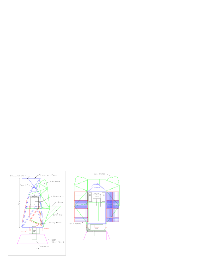
Figure 1: The Boomerang  payload. The extensive shielding prevents stray-light contamination and helps to maintain thermal stability.

The Boomerang telescope (Figure 1) was designed specifically for the harsh conditions of Antarctic ballooning (Crill et al., 2002). The extensive shielding prevents the contamination by stray-light, and protects other sensitive components from the Sun. This is especially important for daytime ballooning over Antarctica, where thermal management is vital. The back of the telescope is constantly illuminated by the Sun, reaching temperatures of $55^{\circ}$ C, while the front is shaded and can cool to less than $-20^{\circ}$ C.

Boomerang scans in azimuth, with the elevation kept constant for at least one hour. Sky rotation turns this one-dimensional azimuthal scan strategy into a cross-linked pattern on the celestial sphere. B98 and BOOM03 both used a differential GPS array, a fixed Sun sensor and rate gyros for pointing reconstruction. For BOOM03, the pointed sun sensor and tracking star camera should improve the pointing reconstruction error.

The Boomerang primary mirror is an off-axis parabola with a diameter of 1.3 m. It is 45^∘ degrees off axis and has a focal length of 1280 mm. The primary feeds a pair of cold re-imaging mirrors which are kept at 1.65 K inside the cryostat (Figure 2). The tertiary forms an image of the primary and acts as the Lyot stop for our system. It controls the illumination on the primary, limiting the effective diameter to about 80 cm. There is a 1 cm hole in the tertiary behind which sits a calibration lamp. It fires once every 15 minutes allowing us to monitor any calibration drift.

Figure 2:  An overview of the Boomerang  optics. Radiation from the primary reflects off the secondary, to the tertiary and then to the focal plane. The secondary and tertiary correct aberrations induced by the primary. They are kept at 1.65 K in a box coated with absorbing material. The tertiary acts as the Lyot stop for the system, controlling the illumination of the primary. Spillover off the edge of the tertiary sees a 1.65 K blackbody.

The Boomerang cryostat can keep the detectors at 0.275 K for 15 days (Masi et al., 1999). Toroidal nitrogen and helium tanks (with the helium tank inside the nitrogen tank) are suspended via 1.6 mm Kevlar ropes. The insert, which contains the cold mirrors and the focal plane, is bolted to the helium tank. The insert also contains a single stage ³He refrigerator which can keep the focal plane at 0.275 K for 12-13 days (Masi et al., 1999). Since the ⁴He and LN₂ stages have a longer hold time (18 and 16 days respectively) than the ³He stage, we added capability for an in-flight cycle of the ³He refrigerator.

3 BOOM03 Receiver

The BOOM03 receiver was designed for measurement of CMB temperature and polarization anisotropies. There are 8 pixels, and each pixel contains two detectors. Four of the pixels contain pairs of polarization sensitive bolometers (PSB’s) operating at 145 GHz. The other four pixels are 2-color photometers operating at 245 and 345 GHz. Both the PSB’s and the photometers use corrugated feed horns. Table 1 summarizes the properties of the BOOM03 receiver. Figure 3 shows the layout of the focal plane projected onto the sky.

Freq	Bandwidth	$\#$Channels	Beam FWHM	Exp. NETCMB
145 GHz	46 GHz	8	$9.5^{\prime}$	160 $\mu K\sqrt{s}$
245 GHz	100 GHz	4	$6.5^{\prime}$	290 $\mu K\sqrt{s}$
345 GHz	100 GHz	4	$7^{\prime}$	660 $\mu K\sqrt{s}$

Table 1: Summary of the properties of the BOOM03 receiver. The FWHM is based on a pre-flight measurement using a tethered thermal source placed 1 km from the telescope. The $NET_{CMB}$ is calculated using a model of our detectors based on pre-flight loadcurve data. Preliminary analysis of flight data provides a similar answer at 145 GHz

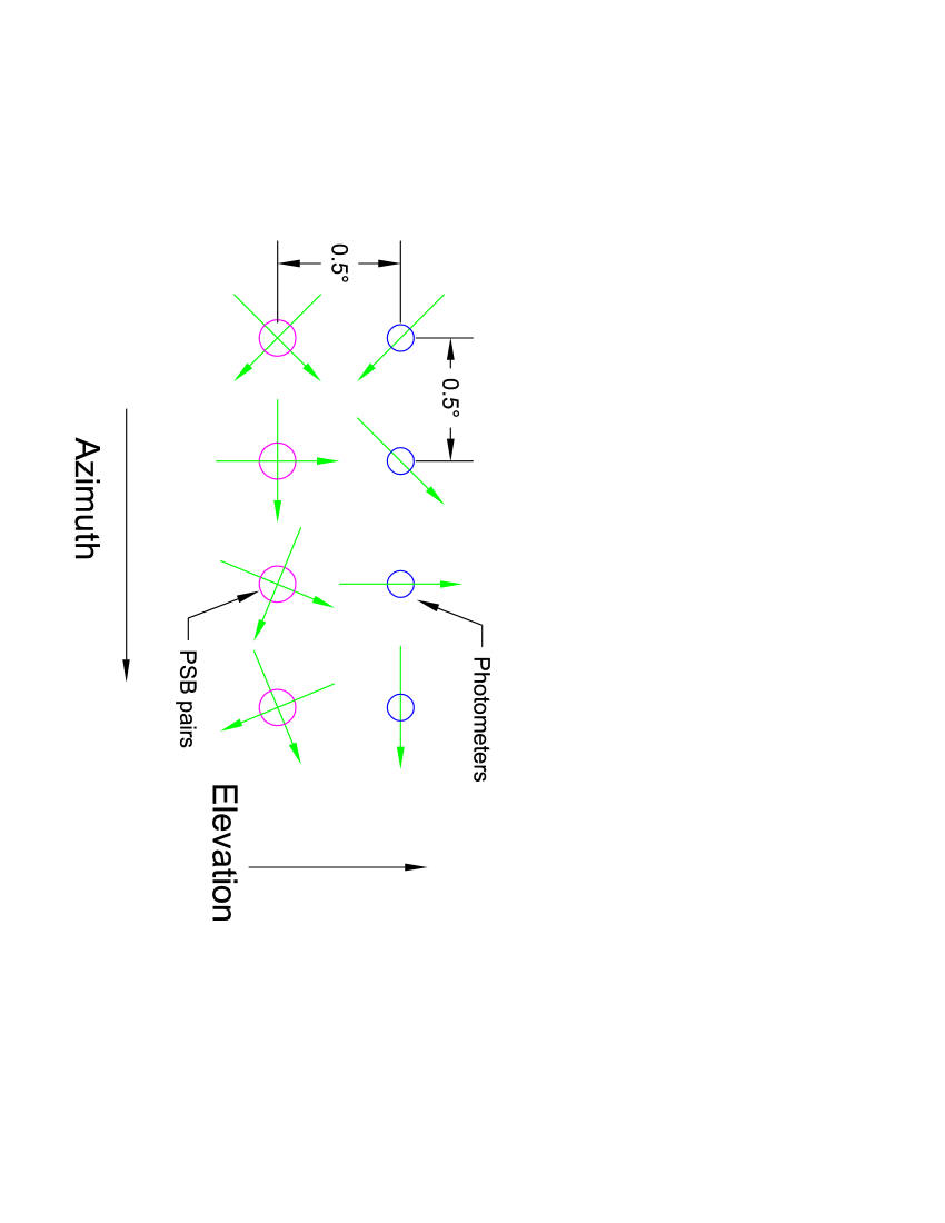
Figure 3: Focal Plane Schematic. 2-color photometers with band centers at 245 GHz and 345 GHz populate the upper row. Each photometer is only sensitive to one polarization. The lower row has 4 pairs of PSB’s. The elements in a PSB pair are sensitive orthogonal polarizations. The circles representing the pixels show relative beams sizes: $\sim 7^{\prime}$ for both photometer channels and $9^{\prime}$ for the PSB’s. The green arrows through the circles show the orientation of the polarization sensitivity. The photometer and PSB rows are separated by $0.5^{\circ}$ in elevation, while the pixels in a row are separated by $0.5^{\circ}$ in cross-elevation.

3.1 Polarization Sensitive Bolometers

The polarization sensitive bolometers are a variation on the original micro-mesh design used in B98 (Jones et al., 2003). Instead of a spider web design, the mesh is a square grid. The grid is only metallized in one direction (Figure 4) making it sensitive to only one component of the incoming electric field. A pair of these with metallized directions oriented $90^{\circ}$ apart are mounted at the end of a corrugated feed structure, separated by $60\mu$m along the axis of propagation. This allows for simultaneous measurement of both electric field components at the same point on the sky, through the same filters and feed structure.

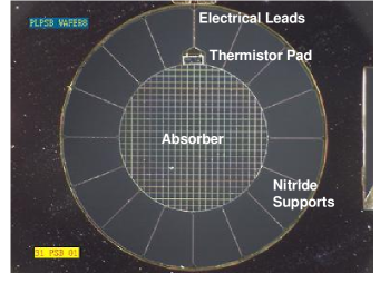
Figure 4: A Polarization Sensitive Bolometer. The diameter of the grid is 2.6 mm. The Si₃N₄ mesh is metallized in the vertical direction only, making the device sensitive to vertical polarization only. The horizontal component of the grid is un-metallized and provides mechanical support for the device. Orthogonally metallized devices are spaced $60\mu$m apart at the exit aperture of a corrugated feed structure.

Figure 5 shows the feed structure for a PSB pair. Light enters into a corrugated back-to-back feed horn, travels out of the back feed horn, across the thermal break and into the filter stack which is mounted on the front of the corrugated reconcentrating feed. The filter stack consists of metal mesh low pass filters which which define the upper edge of the band to be roughly $170$ GHz and a Yoshinaga/Black-poly filter which prevents high frequency leaks. The lower edge of the band is defined by the waveguide cut-off of the back-to-back horn to be $122$ GHz. Once the radiation passes through the filter stack, it enters the reconcentrating feed which couples the radiation to the pair of PSB’s sitting at its exit aperture. The entire feed structure is designed so that polarization is preserved as the radiation travels from the entrance aperture to the bolometers (Jones et al., 2003).

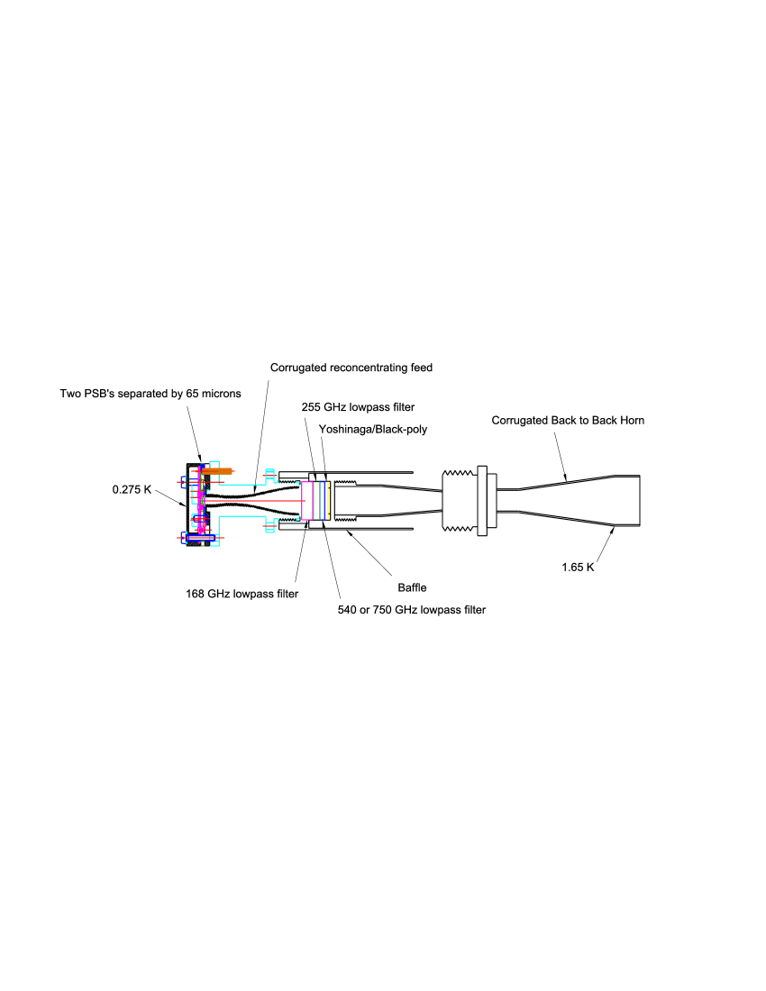
Figure 5: The PSB feed structure. Radiation travels through the back-to-back feed and passes through the filter stack as it enters the reconcentrating feed. The PSB pair sits at the exit aperture of the reconcentrating feed. Both the back-to-back feed and the reconcentrating feed are designed to preserve polarization.

4 Photometers

The 2-color photometer (Figure 6) design has evolved from the 3-color photometer of B98. The photometers operate at 245 and 345 GHz using conventional spider web bolometers. It is fed by a back-to-back corrugated feed which was designed to be single-moded from 180 GHz to nearly 400 GHz. The photometers are made polarization sensitive by placing a polarizing grid in front of feed horn entrance aperture.

Incoming radiation passes through the polarizing grid and into the back-to-back feed horn. It exits the feed horn and enters the photometer body passing through a metal mesh low pass and a Yoshinaga/Black-poly filter. Radiation below 295 GHz is transmitted by the dichroic to the 245 GHz bolometer, and the high frequency radiation is reflected to the 345 GHz bolometer.

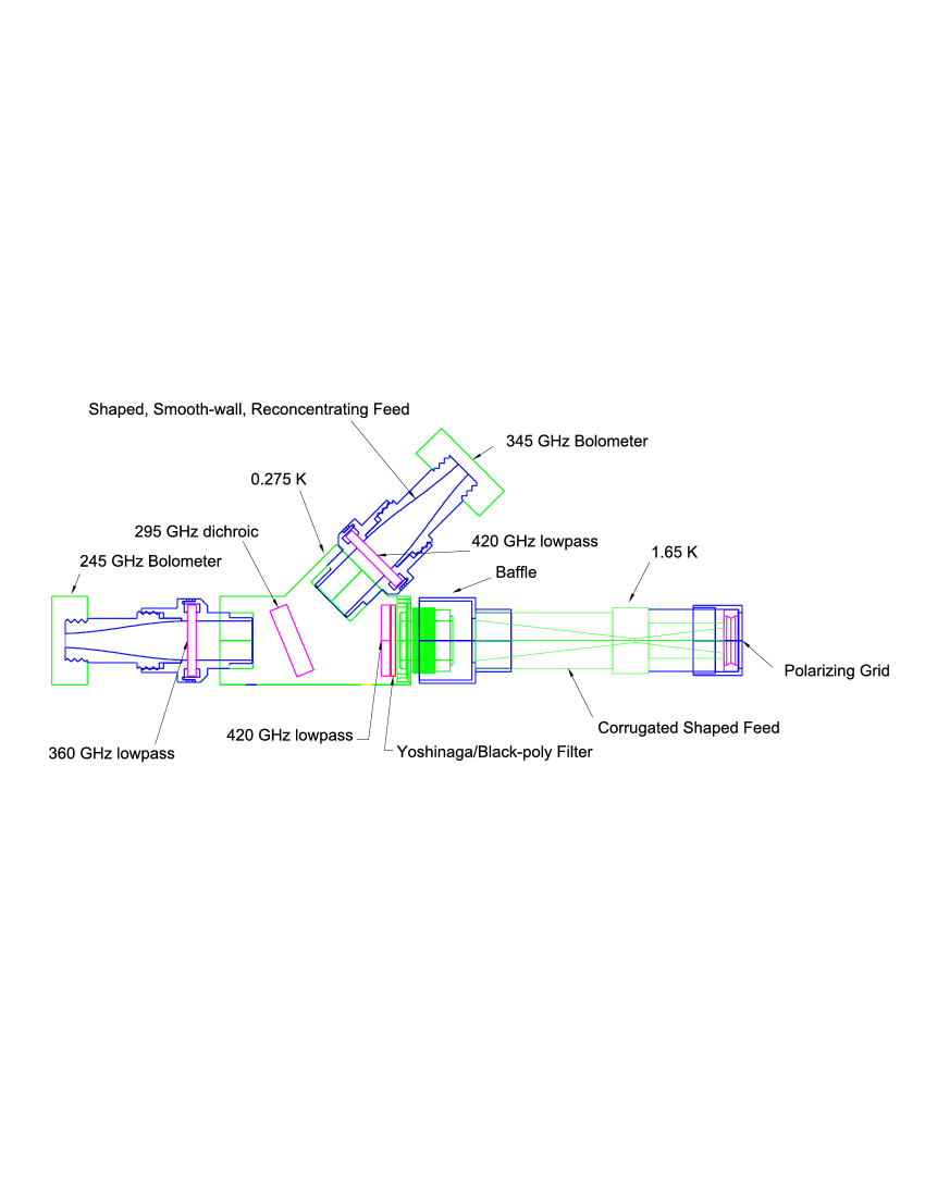
Figure 6: The photometer feed structure. Radiation passes through a polarizing grid mounted in front of the back-to-back feed horn. It exits the feed horn and enters the photometer body passing through a pair of low pass filters. A dichroic transmits frequencies below 295 GHz to the 245 GHz bolometer and reflects high frequency radiation to the 345 GHz bolometer.

5 Measuring Polarization

The Stokes parameters completely describe the polarization state of an electric field. A general polarized electromagnetic wave with angular frequency $\omega=2\pi\nu$ can be described by:

$$\vec{E}=E_{x}(t)sin(\omega t-\delta_{x}(t))\hat{x}+E_{y}(t)sin(\omega t-\delta_{y}(t))\hat{y}.$$ (1)

The Stokes parameters can be written as

$$I = \left<E_{y}^{2}+E_{x}^{2}\right>,$$ (2)

$$Q = \left<E_{x}^{2}-E_{y}^{2}\right>,$$ (3)

$$U = \left<2E_{y}E_{x}\cos(\delta_{y}-\delta_{x})\right>,$$ (4)

$$V = \left<2E_{y}E_{x}\sin(\delta_{y}-\delta_{x})\right>,$$ (5)

$$\tau = \frac{1}{2}\tan^{-1}(\frac{U}{Q}),$$ (6)

where the averaging is done over times scales longer than the period of the wave. The total intensity of the radiation is described by $I$. Parameters $Q$ and $U$ describe the linear polarization, while $V$ quantifies the degree of circular polarization ($V=0$ when the radiation is linearly polarized). $\tau$ is the polarization angle.

Ideally, the signal from one of our detectors is comprised of the total power received in one polarization. For example, the signal received by a detector sensitive to the x-component of the electric field would be proportional to $E_{x}^{2}$. In order to measure $Q$ and $U$, we must combine data from different detectors or multiple rotation angles for a single detector. This issue is complicated by the fact that each of our detectors has a finite cross-polarization ($1\%-10\%$) meaning that our x-polarized detector is contaminated with a small amount of $E_{y}^{2}$.

A single detector with no cross-polarization measures a combination $I$, $Q$ and $U$ in a pixel $p$. The signal is

$$V_{i}^{p} = \gamma_{i}(I^{p}+Q^{p}\cos{(2\alpha)}+U^{p}\sin{(2\alpha})),$$ (7)

$$= \gamma_{i}T_{i}^{p}$$ (8)

where $V_{i}$ is the detector voltage, $\alpha$ is the polarization orientation of the detector, $\gamma_{i}$ is the calibration factor. $I$, $Q$ and $U$ are expressed as deviations from $T_{CMB}$ and $T_{i}^{p}$ is the total signal seen in one polarization. The calibration factor (with units $V/K_{CMB}$) is defined with respect to an unpolarized source. This is consistent with defining CMB temperature and polarization signals as

$$T = \frac{T_{x}+T_{y}}{2},$$ (9)

$$Q = \frac{T_{x}-T_{y}}{2}.$$ (10)

The polarization efficiency can be described as the ratio of the signal in the desired polarization to total signal, for example

$$\rho_{x}=\frac{2\gamma_{x}E_{x}^{2}}{V_{x}},$$ (11)

where $E_{x}^{2}$ is the x-component of the incoming radiation and $V_{x}$ is the signal measured by a detectors with polarization orientation in the $\hat{x}$ direction. If $\rho=1$, there is no cross-polarization. If we rotate a polarized source in front of our detector, then the detector sees a signal

$$S=\beta(1-\rho\sin^{2}(\theta_{det}-\theta_{source})),$$ (12)

where $S=\beta$ when the source and detector have aligned polarizations and $S=\beta(1-\rho)$ when the source and detector are $90^{\circ}$ apart.

To understand the effect of polarization efficiency, it is easiest to consider a PSB pair with polarizations oriented in the $\hat{x}$ and $\hat{y}$ directions. For the general case, we can apply the rotation rules for the Stokes parameters. Including the effects of cross polarization, we have

$$V_{x} = 2\gamma_{x}(E_{x}^{2}+(1-\rho_{x})E_{y}^{2}),$$ (13)

$$V_{y} = 2\gamma_{y}(E_{y}^{2}+(1-\rho_{y})E_{x}^{2}),$$ (14)

which can be re-written as

$$V_{x} = 2\gamma_{x}((1-\frac{\rho_{x}}{2})I+\frac{\rho_{x}}{2}Q),$$ (15)

$$V_{y} = 2\gamma_{y}((1-\frac{\rho_{y}}{2})I-\frac{\rho_{y}}{2}Q).$$ (16)

If we let $\rho_{x}=\rho_{y}=\rho$, then we get a rather simple solution

$$I = \frac{1}{2}\frac{\frac{V_{x}}{\gamma_{x}}+\frac{V_{y}}{\gamma_{y}}}{2-\rho},$$ (17)

$$Q = \frac{1}{2}\frac{\frac{V_{x}}{\gamma_{x}}-\frac{V_{y}}{\gamma_{y}}}{\rho},$$ (18)

illustrating that the cross-polarization causes a loss of efficiency for $Q$ measurement. Since the polarization signal is approximately $10\%$ of the temperature anisotropy signal, the above equations illustrate the importance of high-precision measurements of the gains and polarization efficiencies for each channel.

6 BOOM03 Flight

The second long duration flight of Boomerang was launched on January 6, 2003 from Williams Field at McMurdo Station, Antarctica. The flight lasted for 15 days before it was terminated on January 21. During that time period, we were able to get 11.7 days of good data. We lost 20 hours because the ³He refrigerator ran out at the end of day 11, and we had to recycle it. Also, the payload was losing altitude for most of the flight. At the end of day 13, we had to shutdown the telescope because wind shear at 70,000 ft made attitude control difficult.

Even with the loss of altitude from 120,000 ft to 70,000 ft, the 145 GHz channels were not severely effected. At 75,000 ft, the 145 GHz channels had a responsivity which was approximately $15\%$ less than the peak responsivity, while the 245 and 345 GHz channels had responsivities which were $30\%$ less than their peak value. We did not dip below 95,000 ft until the end of day 11. At 95,000 ft, the 145 GHz channels had only a $5\%$ responsivity loss, while the 245 and 345 GHz channels had a $10\%$ loss.

The scan strategy was designed to balance the effects of sample variance and noise, optimizing our sensitivity to $C_{\ell}^{T}$, $C_{\ell}^{TE}$ and $C_{\ell}^{EE}$. Our entire CMB region covers an area of 1284 deg², slightly larger than the region used for B98 in Ruhl et al. (2002). This region was split into a shallow region of size 1161 deg² and a deep region of size 123 deg². We also spent time observing near the galactic plane in an attempt to characterize foreground polarization. Figure 7 shows a plot of the sky coverage for one 145 GHz detector and Table 2 shows how our observation time was divided.

Region	7’ pixels	Area (deg2)	Average Time (s)
CMB Deep	9397	123	46
CMB Shallow	88547	1161	3.35
CMB Total	97944	1284	7.45
Galaxy	29944	393	4.67

Table 2: A list of the BOOM03 primary scan regions, including the average amount of observation time per pixel per detector. The CMB Total region is the union of the CMB Shallow and CMB Deep regions; the average time per pixel is a bit skewed since the deep region pixels dominate the average.

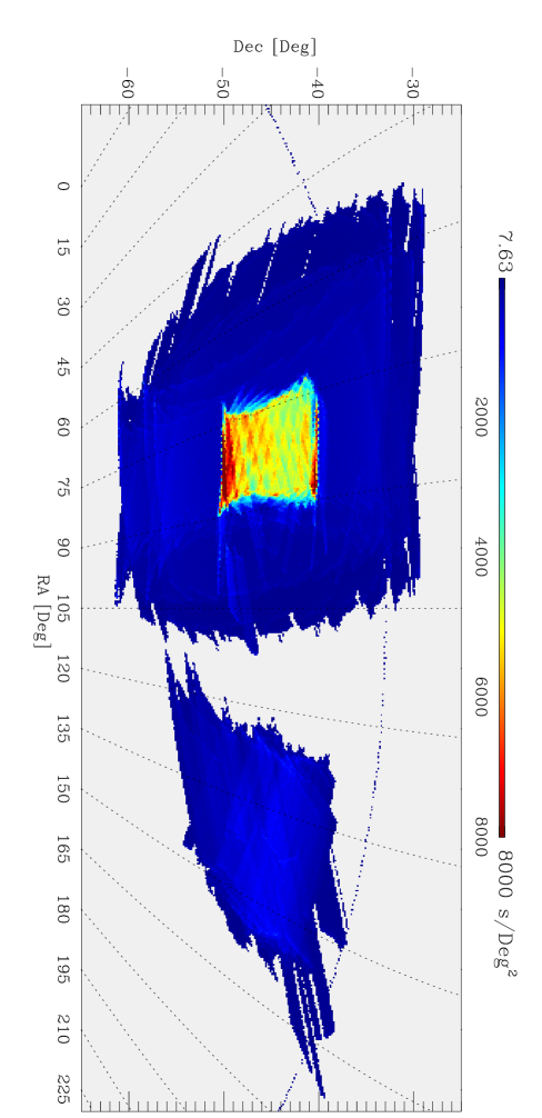
Figure 7: Sky coverage for one element of one PSB pair.

7 Projected Results

With our flight data in hand, we can project our sensitivity to $C_{\ell}^{T}$, $C_{\ell}^{TE}$, and $C_{\ell}^{EE}$. Figure 8 shows what we can expect statistically with eight detectors at 145 GHz. These error bars are estimated using the formulas presented in Zaldarriaga et al. (1997). The combined NET assumes that all channels have an NET${}_{CMB}=160\mu K\sqrt{s}$. No allotment is made for calibration uncertainty, beam uncertainty, pointing error, systematics or the fact that long time constants at 145 GHz will decrease signal-to-noise at high-$\ell$.

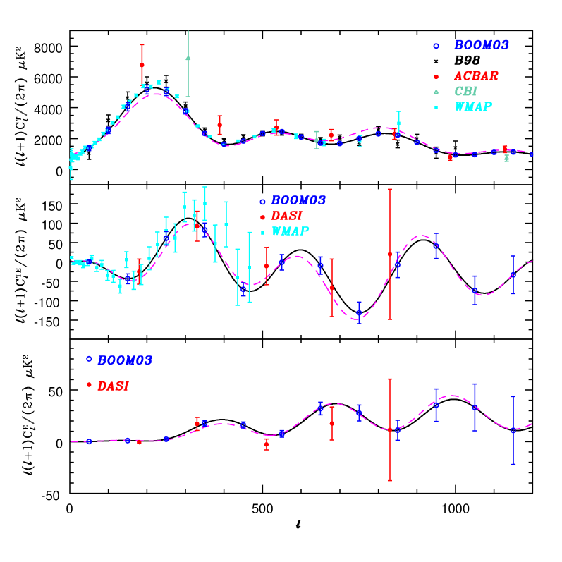
Figure 8: Forecasted results for BOOM03 at 145 GHz compared with recent results from B98 (Ruhl et al., 2002), ACBAR (Kuo et al., 2002), WMAP (Hinshaw et al., 2003), CBI (Mason et al., 2002) and DASI (Kovac et al., 2002). The top panel shows $C_{\ell}^{T}$, the middle shows $C_{\ell}^{TE}$, and the bottom $C_{\ell}^{E}$. The models are best fits to the pre-WMAP data (Goldstein et al., 2002) for a $\Lambda CDM$ model (black line) and a $\Lambda=0$ model (dashed magenta line). This is a statistical calculation assuming that all 8 145 GHz channels have an NET${}_{CMB}=160\mu K\sqrt{s}$. No allotment is made for calibration uncertainty, beam uncertainty, pointing error, systematics or the fact that our long time constants at 145 GHz will decrease signal-to-noise at high-$\ell$.

8 Acknowledgments

The Boomerang project has been supported by NASA, NSF-OPP and NERSC in the U.S., by PNRA, Universitá “La Sapienza” and ASI in Italy, by PPARC in the UK, and by CIAR and NSERC in Canada. T.M. acknowledges support from a NASA GSRP fellowship. The authors would like to thank the National Scientific Balloon Facility (NSBF) and the U.S. Antarctic Program for excellent field and flight support.

References

- (1)
- Crill et al. (2002) B. P. Crill, et al. 2002, astro-ph/0206254, submitted to ApJ
- Goldstein et al. (2002) J. H. Goldstein, et al. 2002, astro-ph/0212517, submitted to ApJ
- Hinshaw et al. (2003) G. Hinshaw, et al. 2003, astro-ph/0302217, submitted to ApJ
- Jones et al. (2003) W. C. Jones, et al. “A Polarization Sensitive Bolometric Receiver for Observations of the Cosmic Microwave Background”, in Proceedings of SPIE Vol. 4855 Millimeter and Submillimeter Detectors for Astronomy, edited by T.G. Phillips, J. Zmuidzinas, (SPIE, Bellingham, WA, 2003) page 227.
- Kogut et al. (2003) A. Kogut, et al. 2003, astro-ph/0302213, submitted to ApJ
- Kovac et al. (2002) J. M. Kovac, E. M. Leitch, C. Pryke, J. E. Carlstrom, N. W. Halverson, and W. L. Holzapfel. Nature, 420:772–787, December 2002.
- Kuo et al. (2002) C. L. Kuo, et al. 2002, astro-ph/0212289, submitted to ApJ
- Masi et al. (1998) S. Masi et al., Cryogenics, 38:319, 1998.
- Masi et al. (1999) S. Masi et al., Cryogenics, 39:217, 1999.
- Mason et al. (2002) B. Mason, et al. 2002, astro-ph/0205384, ApJ in press
- Ruhl et al. (2002) J. E. Ruhl, et al. 2002, astro-ph/0212229, submitted to ApJ
- Zaldarriaga et al. (1997) M. Zaldarriaga, D. N. Spergel, and U. Seljak. ApJ, 488:1, October 1997.