Transition from collisionless to collisional MRI

Abstract

Recent calculations by Quataert et al. (2002) found that the growth rates of the magnetorotational instability (MRI) in a collisionless plasma can differ significantly from those calculated using MHD. This can be important in hot accretion flows around compact objects. In this paper we study the transition from the collisionless kinetic regime to the collisional MHD regime, mapping out the dependence of the MRI growth rate on collisionality. A kinetic closure scheme for a magnetized plasma is used that includes the effect of collisions via a BGK operator. The transition to MHD occurs as the mean free path becomes short compared to the parallel wavelength $2\pi/k_{\parallel}$. In the weak magnetic field regime where the Alfvén and MRI frequencies $\omega$ are small compared to the sound wave frequency $k_{\parallel}c_{0}$, the dynamics are still effectively collisionless even if $\omega\ll\nu$, so long as the collision frequency $\nu\ll k_{\parallel}c_{0}$; for an accretion flow this requires $\nu\mathrel{\mathchoice{\vbox{\offinterlineskip\halign{$\m@th\displaystyle\hfil#\hfil$\cr<\crcr\sim\crcr} }}{\vbox{\offinterlineskip\halign{$\m@th\textstyle\hfil#\hfil$\cr<\crcr\sim\crcr} }}{\vbox{\offinterlineskip\halign{$\m@th\scriptstyle\hfil#\hfil$\cr<\crcr\sim\crcr} }}{\vbox{\offinterlineskip\halign{$\m@th\scriptscriptstyle\hfil#\hfil$\cr<\crcr\sim\crcr} }}}\Omega\sqrt{\beta}$. The low collisionality regime not only modifies the MRI growth rate, but also introduces collisionless Landau or Barnes damping of long wavelength modes, which may be important for the nonlinear saturation of the MRI.

1 Introduction

Balbus & Hawley (1991) showed that the magnetorotational instability (MRI), a local instability of differentially rotating magnetized plasmas, is the most efficient source of angular momentum transport in many astrophysical accretion flows (see Balbus & Hawley 1998 for a review). The MRI may also be important for dynamo generation of galactic and stellar magnetic fields. Most studies of the MRI have employed standard MHD equations which are appropriate for collisional, short mean free path plasmas. Recently, however, Quataert, Dorland $\&$ Hammett (2002; hereafter QDH) studied the MRI in the collisionless regime using the kinetic results of Snyder, Hammett $\&$ Dorland (1997). They showed that the MRI persists as a robust instability in a collisionless plasma, but that at high $\beta\gg 1$ (ratio of plasma pressure to magnetic pressure), the physics of the instability is quite different and the kinetic growth rates can differ significantly from the MHD growth rates.

One motivation for studying the MRI in the collisionless regime is to understand radiatively inefficient accretion flows onto compact objects. An example of non-radiative accretion is the radio and X-ray source Sagittarius A^∗, which is thought to be powered by gas accreting onto a supermassive black hole at the center of our galaxy (see Quataert 2003 for a review). In radiatively inefficient accretion flow models, the accreting gas is a hot, low density, plasma, with the proton temperature large compared to the electron temperature ($T_{p}\approx 10^{12}$ K $\gg T_{e}\approx 10^{10}-10^{11}$ K). In order to maintain such a two-temperature configuration, the accretion flow must be collisionless in the sense that the timescale for electrons and protons to exchange energy by Coulomb collisions is longer than the inflow time of the gas (for models of Sagittarius A*, the collision time close to the black hole is $\approx 7$ orders of magnitude longer than the inflow time).

In this paper we extend the kinetic results of QDH to include collisions; we study the behavior of the MRI in the transition from the collisionless regime to the collisional MHD regime. Instead of using a more accurate but very complicated Landau or Balescu-Lenard collision operator, we use a simpler Bhatnagar-Gross-Krook (BGK) collision operator (Bhatnagar, Gross $\&$ Krook 1954) that conserves number, momentum and energy.

There are several reasons for studying the behavior of the MRI with collision frequency: (1) one gains additional understanding of the qualitatively different physics in the MHD and kinetic regimes, (2) one of the key differences between the MRI in kinetic theory and MHD is the anisotropic (with respect to the local magnetic field) pressure response in a collisionless plasma (QDH). Even if particle collisions are negligible, high frequency waves with frequencies $\sim$ the proton cyclotron frequency may tend to isotropize the proton distribution function. Our treatment of “collisions” can qualitatively describe this process as well; and (3) the transition from the collisional to the kinetic MRI could be dynamically interesting if accretion disks undergo transitions from thin disks to hot radiatively inefficient flows (as has been proposed to explain, e.g., state changes in X-ray binaries; Esin et al. (1997)). For example, there could be associated changes in the rate of angular momentum transport ($\alpha$).

The paper is organized as follows. In the next section (§2) we briefly discuss the linearized kinetic equations in the long-wavelength, low frequency limit (the “MHD” limit); this is a review of the formalism used by QDH. In $\S$3 we then derive the kinetic equation for the perturbed pressure including effects of proton-proton collisions via a BGK operator; this result is needed to “close” our basic equations and derive the dispersion relation for the plasma. In $\S$4 we discuss simpler Landau-fluid (Snyder et al. 1997) closure schemes for deriving the perturbed pressure. The Landau-fluid closure approximations agree well with the exact kinetic results from §3 in the low and high collisionality regimes and provide a smooth transition for intermediate regimes. In $\S$5 we numerically solve for the growth rate of the kinetic MRI and discuss the effects of collisions. Finally in $\S$6 we summarize our results and discuss their astrophysical implications.

2 Linearized Kinetic-MHD Equations

The analysis in this paper is restricted to fluctuations that have wavelengths much larger than proton Larmor radius and frequencies well below the proton cyclotron frequency. In this limit, a plasma can be described by the following magneto-fluid equations(Kruskal & Oberman, 1958; Rosenbluth & Rostoker, 1959; Kulsrud, 1983):

$$\frac{\partial\rho}{\partial t}+\nabla\cdot\left(\rho{\bf V}\right)=0,$$ (4)

$$\rho\frac{\partial{\bf V}}{\partial t}+\rho\left({\bf V}\cdot\nabla\right){\bf V}=\frac{\left(\nabla\times{\bf B}\right)\times{\bf B}}{4\pi}-\nabla\cdot{\bf P}+{\bf F_{g}},$$

$$\frac{\partial{\bf B}}{\partial t}=\nabla\times\left({\bf V}\times{\bf B}\right),$$

$${\bf P}=p_{\perp}{\bf I}+\left(p_{\parallel}-p_{\perp}\right){\bf\hat{b}\hat{b}},$$

where $\rho$ is the mass density, ${\bf V}$ is the fluid velocity, ${\bf B}$ is the magnetic field, ${\bf F_{g}}$ is the gravitational force, ${\bf\hat{b}}={\bf B}/|{\bf B}|$ is a unit vector in the direction of the magnetic field, and ${\bf I}$ is the unit tensor. In equation (4) an ideal Ohm’s law is used, neglecting effects such as resistivity. ${\bf P}$ is the pressure tensor that has different perpendicular ($p_{\perp}$) and parallel ($p_{\parallel}$) components with respect to the background magnetic field (unlike in MHD, where there is only a scalar pressure). The pressures are determined by solving the drift kinetic equation given below. ${\bf P}$ should in general be a sum over all species but in the limit where ion dynamics dominate and electrons just provide a neutralizing background, the pressure can be interpreted as the ion pressure. This is the case for hot accretion flows in which $T_{p}\gg T_{e}$.

We assume that the background (unperturbed) plasma is described by a non-relativistic Maxwellian distribution function with equal parallel and perpendicular pressures (temperatures). Although the equilibrium pressure is assumed to be isotropic, the perturbed pressure is not. We take the plasma to be differentially rotating, but otherwise uniform (we neglect temperature and density gradients). Equilibrium analysis for equation (4) in presence of a subthermal magnetic field with vertical ($B_{z}=B_{0}\sin\theta$) and azimuthal ($B_{\phi}=B_{0}\cos\theta$) components gives a Keplerian rotation ($\Omega\propto R^{-3/2}$) provided the magnetic field is sufficiently weak ($B_{0}^{2}\ll GM_{0}\rho_{0}/R$, where $M_{0}$ is the mass of the central object).

In a differentially rotating plasma, a finite $B_{R}$ leads to a time-dependent $B_{\phi}$, which greatly complicates the kinetic analysis (unlike in MHD, where a time-dependent $B_{\phi}$ can be accounted for; Balbus $\&$ Hawley 1991); we therefore set $B_{R}=0$. For linearization we consider fluctuations of the form $\exp[-i\omega t+i{\bf k}\cdot{\bf x}]$, with ${\bf k}=k_{R}\hat{R}+k_{z}\hat{z}$, i.e., axisymmetric modes; we also restrict our analysis to local perturbations for which $|{\bf k}|R\gg 1$. Writing $\rho=\rho_{0}+\delta\rho$, ${\bf B}={\bf B_{0}}+\delta{\bf B}$, $p_{\perp}=p_{0}+\delta p_{\perp}$, and $p_{\parallel}=p_{0}+\delta p_{\parallel}$, ${\bf V}=\hat{\phi}\Omega R+\delta{\bf v}$ (with Keplerian rotation $\Omega(R)$), and working in cylindrical coordinates, the linearized versions of equations (4)-(4) become (QDH):

$$\omega\delta\rho=\rho_{0}{\bf k}\cdot\delta{\bf v},$$ (7)

$$-i\omega\rho_{0}\delta v_{R}-\rho_{0}2\Omega\delta v_{\phi}=-\frac{ik_{R}}{4\pi}\left(B_{z}\delta B_{z}+B_{\phi}\delta B_{\phi}\right)+\frac{ik_{z}B_{z}\delta B_{R}}{4\pi}-ik_{R}\delta p_{\perp},$$

$$-i\omega\rho_{0}\delta v_{\phi}+\rho_{0}\delta v_{R}\frac{\kappa^{2}}{2\Omega}=\frac{ik_{z}B_{z}\delta B_{\phi}}{4\pi}-ik_{z}\sin\theta\cos\theta[\delta p_{\parallel}-\delta p_{\perp}],$$

$$-i\omega\rho_{0}\delta v_{z}=-\frac{ik_{z}B_{\phi}\delta B_{\phi}}{4\pi}-ik_{z}[\sin^{2}\theta\delta p_{\parallel}+\cos^{2}\theta\delta p_{\perp}],$$ (11)

$$\omega\delta B_{R}=-k_{z}B_{z}\delta v_{R},$$

$$\omega\delta B_{\phi}=-k_{z}B_{z}\delta v_{\phi}-\frac{ik_{z}B_{z}}{\omega}\frac{d\Omega}{d\ln R}\delta v_{R}+B_{\phi}{\bf k}\cdot\delta{\bf v},$$

$$\omega\delta B_{z}=k_{R}B_{z}\delta v_{R},$$

where $\kappa^{2}=4\Omega^{2}+d\Omega^{2}/d\ln R$ is the epicyclic frequency. To complete our system of equations and derive the dispersion relation for linear perturbations, we need expressions for $\delta p_{\perp}$ and $\delta p_{\parallel}$. These can be obtained by taking moments of the linearized and Fourier transformed drift-kinetic equation that includes a linearized BGK collision operator. The drift-kinetic MHD model is described by Kulsrud (1983) based on earlier work by Kruskal $\&$ Oberman (1958) and Rosenbluth & Rostoker (1959). The drift-kinetic equation for the distribution function including the effects of gravity is

$$\frac{\partial f}{\partial t}+\left(v_{\parallel}{\bf\hat{b}}+{\bf v}_{E}\right)\cdot\nabla f+\left(-{\bf\hat{b}}\cdot\frac{D{\bf v}_{E}}{Dt}-\mu{\bf\hat{b}}\cdot\nabla B+\frac{e}{m}(E_{\parallel}+F_{g\parallel}/e)\right)\frac{\partial f}{\partial v_{\parallel}}=C\left(f\right),$$ (12)

where ${\bf v}_{E}=c\left({\bf E}\times{\bf B}\right)/B^{2}$, $\mu=({\bf v}_{\perp}-{\bf v}_{E})^{2}/2B$ is the magnetic moment (conserved in our approximations in the absence of collisions), $F_{g\parallel}=GM_{0}m\hat{R}\cdot\hat{\bf b}/R^{2}$, and $D/Dt=\partial/\partial t+\left(v_{\parallel}{\bf\hat{b}}+{\bf v}_{E}\right)\cdot\nabla$. The fluid velocity ${\bf V}={\bf v}_{E}+{\bf\hat{b}}u_{\parallel}$, so the $E\times B$ drift ${\bf v}_{E}$ is determined by the perpendicular component of equation (4). [Only the $E\times B$ drift appears directly in equation (12). Other drifts such as the grad B, curvature, or gravity $\times B$ drifts are higher order in the MHD drift kinetic ordering (Kulsrud 1983), which assumes the frequencies are low compared to the cyclotron frequency and the gyroradius small compared to gradient scale lengths. On the other hand, the parallel component of the gravitational force $F_{g\parallel}$ is included as it can be the same order as the parallel electric field, which is small compared to the perpendicular electric field in ideal MHD.] Note the addition of a collision operator on the right hand side of the kinetic equation to allow for generalization to collisional regimes. In the next section we derive the linearly-exact kinetic expressions for $\delta p_{\parallel}$ and $\delta p_{\perp}$ using the BGK collision operator in equation (12). We then compare these with closure approximations from Snyder et al. (1997).

3 Kinetic Closure Including Collisions

In this section we use a simple BGK collision operator (Bhatnagar et al. 1954) to calculate $\delta p_{\parallel}$ and $\delta p_{\perp}$ from equation (12). Since we consider only ion-ion collisions, the BGK operator is $C_{K}\left(f\right)=-\nu\left(f-F_{M}\right)$ where $\nu$ is the ion-ion collision frequency and $F_{M}$ is a shifted Maxwellian with the same density, momentum and energy as $f$ (so that collisions conserve number, momentum, and energy). The integro-algebraic BGK operator greatly simplifies the calculations while adequately modeling many of the key properties of the full integro-differential collision operator. In some situations the effects of weak collisions can be enhanced in a more complete collision operator due to sharp velocity gradients in the distribution function. We leave investigation of such effects to future work. In this section, we calculate the linearization of the drift-kinetic equation around an accretion disk equilibrium including equilibrium flows and gravity. It turns out that a number of complicating intermediate terms end up cancelling, and the final forms of the closures used (from equations (26-27) onwards) are identical to what one would get from perturbing around a simple stationary slab equilibrium. We carried out the more detailed calculation to verify that there were no missing terms in the final closures.

The equilibrium distribution function $f_{0}$ is given by

$$f_{0}=\frac{n_{0}}{(2\pi T_{0}/m)^{3/2}}\exp\left(-\frac{m}{2T_{0}}|{\bf v}-{\bf V}_{0}|^{2}\right),$$ (13)

where ${\bf V}_{0}={\bf v}_{E0}+u_{\parallel 0}\hat{{\bf b_{0}}}$ is equal to the Keplerian rotation velocity in $\hat{\phi}$ direction. Since $|{\bf v}-{\bf V}_{0}|^{2}=(v_{\parallel}-u_{\parallel 0})^{2}+2\mu B_{0}$, $f_{0}$ can be expressed in terms of $\left(\mu,v_{\parallel}\right)$ as

$$f_{0}=\frac{n_{0}}{\left(2\pi T_{0}/m\right)^{3/2}}\exp\left(-\frac{m}{2T_{0}}\left((v_{\parallel}-u_{\parallel 0})^{2}+2\mu B_{0}\right)\right).$$ (14)

We shall linearize the drift-kinetic equation and the BGK collision operator. The distribution function is given as $f=f_{0}+\delta f$ where $\delta f$ is the perturbation in the distribution function. The shifted Maxwellian that appears in the BGK collision operator is given by

$$F_{M}=\frac{N_{M}}{\left(2\pi T_{M}/m\right)^{3/2}}\exp{\left\{-\frac{m}{2T_{M}}\left(\left(v_{\parallel}-u_{\parallel M}\right)^{2}+2\mu B\right)\right\}}.$$ (15)

$F_{M}$ has three free parameters ($N_{M}$, $u_{\parallel M}$, $T_{M}$) which are to be chosen so as to conserve number, parallel momentum and energy. When taking moments of the BGK operator, it is important to note that $\int d^{3}v=\int 2\pi\left(B_{0}+\delta B\right)d\mu dv_{\parallel}$. From equation (15) and conservation of number, momentum and energy it follows that

$$N_{M} = n_{0}+\delta n\approx n_{0}\left(1+\frac{\delta B}{B_{0}}\right)+2\pi B_{0}\int d\mu dv_{\parallel}\delta f,$$ (16)

$$N_{M}u_{\parallel M} = N_{M}(u_{\parallel 0}+\delta u)\approx n_{0}u_{\parallel 0}\left(1+\frac{\delta B}{B_{0}}\right)+2\pi B_{0}\int d\mu dv_{\parallel}\delta fv_{\parallel},$$ (17)

$$N_{M}T_{M} = p_{0}+\delta p=p_{0}+(\delta p_{\parallel}+2\delta p_{\perp})/3,$$ (18)

$$\delta p_{\parallel} \approx p_{0}\delta B/B_{0}+2\pi B_{0}\int d\mu dv_{\parallel}\delta fm(v_{\parallel}-u_{\parallel 0})^{2},$$ (19)

$$\delta p_{\perp} \approx 2p_{0}\delta B/B_{0}+2\pi B_{0}\int d\mu dv_{\parallel}\delta f\mu mB_{0},$$ (20)

where the approximate expressions retain only linear terms in perturbed quantities. Linearizing the expression for the relaxed Maxwellian in equation (15) about $f_{0}$, the drift-kinetic BGK collision operator is given by

$$C_{K}\left(\delta f\right)=-\nu\delta f+\nu f_{0}\times$$

$$\left\{\left(\frac{\delta n}{n_{0}}-\frac{3\delta T}{2T_{0}}\right)+\frac{m}{T_{0}}\left(\left(v_{\parallel}-u_{\parallel 0}\right)\delta u+\left(v_{\parallel}-u_{\parallel 0}\right)^{2}\frac{\delta T}{2T_{0}}\right)-\frac{m\mu B_{0}}{T_{0}}\left(\frac{\delta B}{B_{0}}-\frac{\delta T}{T_{0}}\right)\right\}.$$ (21)

The drift-kinetic equation including the BGK operator can be linearized to obtain the following equation for $\delta f$

$$\delta f=u_{\phi 0}(v_{\parallel}-u_{\parallel 0})f_{0}\sin{\theta}\frac{\left(\delta B_{\phi}\sin{\theta}-\delta B_{z}\cos{\theta}\right)m}{T_{0}B_{0}}+\frac{m\left(v_{\parallel}-u_{\parallel 0}\right)f_{0}}{T_{0}\left(-i\omega+ik_{\parallel}\left(v_{\parallel}-u_{\parallel 0}\right)+\nu\right)}\times$$

$$\left(-ik_{\parallel}\mu\delta B+\frac{\left(eE_{\parallel}+F_{g\parallel}\right)}{m}\right)+\frac{\nu f_{0}}{\left(-i\omega+ik_{\parallel}\left(v_{\parallel}-u_{\parallel 0}\right)+\nu\right)}\times$$

$$\left(\frac{\delta n}{n_{0}}-\frac{3}{2}\frac{\delta T}{T_{0}}+\frac{m(v_{\parallel}-u_{\parallel 0})\delta u}{T_{0}}+\frac{m(v_{\parallel}-u_{\parallel 0})^{2}}{2T_{0}}\frac{\delta T}{T_{0}}+\frac{m\mu B_{0}}{T_{0}}\frac{\delta T}{T_{0}}-\frac{m\mu\delta B}{T_{0}}\right),$$ (22)

where $F_{g\parallel}=GM_{0}m\delta B_{R}/B_{0}R^{2}$ is the component of gravitational force in the direction of magnetic field. Choosing a compact notation where $-i\omega\sin{\theta}\left(\delta B_{\phi}\sin{\theta}-\delta B_{z}\cos{\theta}\right)mu_{\phi 0}/eB_{0}$ $+F_{g\parallel}/e+E_{\parallel}\rightarrow E_{\parallel}$, the moments of the perturbed distribution function $\delta f$ in drift coordinates $(v_{\parallel},\mu)$, $\int\left(1,2\mu B_{0},(v_{\parallel}-u_{\parallel 0})^{2}\right)\delta f2\pi B_{0}d\mu dv_{\parallel}$ give

$$\frac{\delta n}{n_{0}}=\frac{\delta B}{B_{0}}\left(1-R\right)+\frac{eE_{\parallel}}{ik_{\parallel}T_{0}}R-\zeta_{2}\left\{\left(\frac{\delta n}{n_{0}}-\frac{3}{2}\frac{\delta T}{T_{0}}\right)Z+\left(\frac{\delta T}{T_{0}}-\frac{\delta B}{B_{0}}\right)Z\right.$$

$$\left.+\sqrt{2}\frac{\delta u}{c_{0}}R+\left(\frac{\delta T}{T_{0}}+2i\sin{\theta}\frac{k_{\parallel}u_{\phi 0}}{\nu}\frac{\left(\delta B_{\phi}\sin{\theta}-\delta B_{z}\cos{\theta}\right)}{B_{0}}\right)\zeta R\right\},$$ (23)

$$\frac{\delta p_{\perp}}{p_{0}}=2\frac{\delta B}{B_{0}}\left(1-R\right)+\frac{eE_{\parallel}}{ik_{\parallel}T_{0}}R-\zeta_{2}\left\{\left(\frac{\delta n}{n_{0}}-\frac{3}{2}\frac{\delta T}{T_{0}}\right)Z+2\left(\frac{\delta T}{T_{0}}-\frac{\delta B}{B_{0}}\right)Z\right.$$

$$\left.+\sqrt{2}\frac{\delta u}{c_{0}}R+\left(\frac{\delta T}{T_{0}}+2i\sin{\theta}\frac{k_{\parallel}u_{\phi 0}}{\nu}\frac{\left(\delta B_{\phi}\sin{\theta}-\delta B_{z}\cos{\theta}\right)}{B_{0}}\right)\zeta R\right\},$$ (24)

$$\frac{\delta p_{\parallel}}{p_{0}}=-2\frac{\delta B}{B_{0}}\zeta^{2}R+\frac{eE_{\parallel}}{ik_{\parallel}T_{0}}\left(1+2\zeta^{2}R\right)-\zeta_{2}\left\{2\left(\frac{\delta n}{n_{0}}-\frac{3}{2}\frac{\delta T}{T_{0}}\right)\zeta R+2\left(\frac{\delta T}{T_{0}}-\frac{\delta B}{B_{0}}\right)\zeta R\right.$$

$$+\left.\sqrt{2}\frac{\delta u}{c_{0}}\left(1+2\zeta^{2}R\right)+\left(\frac{\delta T}{T_{0}}+2i\sin{\theta}\frac{k_{\parallel}u_{\phi 0}}{\nu}\frac{\left(\delta B_{\phi}\sin{\theta}-\delta B_{z}\cos{\theta}\right)}{B_{0}}\right)\zeta\left(1+2\zeta^{2}R\right)\right\}.$$ (25)

$E_{\parallel}$ can be eliminated by taking appropriate combinations of these three equations:

$$\frac{\delta\rho}{\rho_{0}}-\frac{\delta p_{\perp}}{p_{0}}=-\frac{\delta B}{B_{0}}\left(1-R\right)+\zeta_{2}Z\left(\frac{\delta T}{T_{0}}-\frac{\delta B}{B_{0}}\right),$$ (26)

and

$$\left(1+2\zeta^{2}R\right)\frac{\delta\rho}{\rho_{0}}-R\frac{\delta p_{\parallel}}{p_{0}}=\frac{\delta B}{B_{0}}\left(1+2\zeta^{2}R-R\right)-\zeta_{2}\left(Z-2\zeta R\right)\left(\frac{\delta\rho}{\rho_{0}}-\frac{\delta T}{2T_{0}}-\frac{\delta B}{B_{0}}\right),$$ (27)

where $\delta T=\left(2\delta T_{\perp}+\delta T_{\parallel}\right)/3$, $\delta B={\bf\hat{b}_{0}}\cdot\delta{\bf B}$, $\zeta=\left(\omega+i\nu\right)/\sqrt{2}|k_{\parallel}|c_{0}$, $\zeta_{2}=i\nu/\sqrt{2}|k_{\parallel}|c_{0}$, $k_{\parallel}={\bf\hat{b}_{0}\cdot k}$, $T_{\parallel,\perp}=mp_{\parallel,\perp}/\rho$, and $c_{0}=\sqrt{T_{0}/m}$ is the isothermal sound speed of the ions. In equations (26) and (27), $R=1+\zeta Z$ is the plasma response function, where

$$Z\left(\zeta\right)=\frac{1}{\sqrt{\pi}}\int dx\frac{\exp[-x^{2}]}{x-\zeta}$$ (28)

is the plasma dispersion function (NRL plasma formulary 2000). Equations (26) and (27) can be substituted into the linearized fluid equations in §2 to derive the dispersion relation for the plasma. The full closures are, however, very complicated, so it is useful to consider several simplifying limits that isolate much of the relevant physics. In addition, the solution of the MHD equations from §2 with fully kinetic closures will give an implicit equation for the growth rate (involving the $Z$ function) that would have to be solved numerically.

The closure equations can be simplified in two limits, $|\zeta|\ll 1$, the collisionless limit, and $|\zeta|\gg 1$, the high collisionality limit. The derivation of the asymptotic solution for the closure equations in these two limits is given in the Appendix. For high collisionality

$$\frac{\delta p_{\perp}}{p_{0}}=\frac{5}{3}\frac{\delta\rho}{\rho_{0}}+\frac{\zeta_{1}}{\zeta_{2}}\left(\frac{4}{3}+\frac{5}{9\zeta_{1}^{2}}\right)\frac{\delta\rho}{\rho_{0}}-2\frac{\zeta_{1}}{\zeta_{2}}\frac{\delta B}{B_{0}},$$ (29)

and

$$\frac{\delta p_{\parallel}}{p_{0}}=\frac{5}{3}\frac{\delta\rho}{\rho_{0}}+\frac{\zeta_{1}}{\zeta_{2}}\left(-\frac{2}{3}+\frac{5}{9\zeta_{1}^{2}}\right)\frac{\delta\rho}{\rho_{0}}+\frac{\zeta_{1}}{\zeta_{2}}\frac{\delta B}{B_{0}},$$ (30)

where $\zeta_{1}=\omega/\sqrt{2}|k_{\parallel}|c_{0}$. Notice that in the limit that the collision frequency is very high, $\zeta_{2}\rightarrow\infty$, and one recovers the MHD result that the perturbations are adiabatic and isotropic: $\delta p_{\parallel}/p_{0}=\delta p_{\perp}/p_{0}=5\delta\rho/3\rho_{0}$. Inspection of equations (29) and (30) suggests that the MHD limit will be reached whenever $|\zeta_{1}/\zeta_{2}|\ll 1$, i.e., $\nu\gg\omega$. Later we shall show that in fact $\nu\gg\sqrt{2}|k_{\parallel}|c_{0}$ is required, i.e., the collision time must be much less than the sound crossing time of the wavelength of the mode. This is important because the MRI has $\omega\ll|k_{\parallel}|c_{0}$ in a high $\beta$ plasma so the regime $\omega\ll\nu\ll|k_{\parallel}|c_{0}$ is an interesting one.

For low collisionality, $|\zeta|\ll 1$, to second order in $\zeta$,

$$\frac{\delta p_{\perp}}{p_{0}}=\frac{\delta\rho}{\rho_{0}}-i\sqrt{\pi}\zeta_{1}\frac{\delta B}{B_{0}}-\frac{\pi\zeta_{1}\zeta_{2}}{3}\frac{\delta\rho}{\rho_{0}}+\zeta_{1}\zeta_{2}\left(2-\frac{\pi}{3}\right)\frac{\delta B}{B_{0}},$$ (31)

and

$$\frac{\delta p_{\parallel}}{p_{0}} = \frac{\delta\rho}{\rho_{0}}-i\sqrt{\pi}\zeta_{1}\left(\frac{\delta\rho}{\rho_{0}}-\frac{\delta B}{B_{0}}\right)+\frac{\delta\rho}{\rho_{0}}\left(4\zeta_{1}\zeta_{2}-\pi\zeta_{1}^{2}-\frac{7\pi\zeta_{1}\zeta_{2}}{6}\right)+$$ (32)

$$\frac{\delta B}{B_{0}}\left(\sqrt{\pi}\zeta_{1}\zeta_{2}-\frac{\pi\zeta_{1}\zeta_{2}}{6}-2\zeta^{2}-4\zeta_{2}\zeta\right).$$

To first order, there is no effect of collisions on the growth rate of the MRI; the results above are then exactly same as equations (20) and (21) in QDH (who neglected collisions entirely). Collisional effects modify the closure only at order $\zeta^{2}$, though one has to go to this order to find the first order dependence of $\omega$ on $\nu$ in the dispersion relation.

4 Comparison with Landau-Fluid Closures

The results from the last section provide useful expressions for $\delta p_{\perp}$ and $\delta p_{\parallel}$ in the low and high collisionality regimes, $|\zeta|\ll 1$ and $|\zeta|\gg 1$, but it would be convenient to have a single set of equations that can provide a robust transition between these two regimes. The Snyder et al. (1997) closure approximations, which we discuss in this section, can do this.

The second moments of the drift kinetic equation (eq. [12]) yield evolution equations for $\delta p_{\perp}$ and $\delta p_{\parallel}$ (see, e.g., eqs. [16]-[17] of Snyder et al. 1997). The linearized versions of these equations, including a BGK collision operator, are given by

$$-i\omega\delta p_{\parallel}+p_{0}i{\bf k\cdot\delta v}+ik_{\parallel}q_{\parallel}+2p_{0}ik_{\parallel}\delta v_{\parallel}-3p_{0}\Omega\cos{\theta}\frac{\delta B_{R}}{B_{0}}=-\frac{2}{3}\nu\left(\delta p_{\parallel}-\delta p_{\perp}\right),$$ (33)

and

$$-i\omega\delta p_{\perp}+2p_{0}i{\bf k\cdot\delta v}+ik_{\parallel}q_{\perp}-p_{0}ik_{\parallel}\delta v_{\parallel}+\frac{3}{2}p_{0}\Omega\cos{\theta}\frac{\delta B_{R}}{B_{0}}=-\frac{1}{3}\nu\left(\delta p_{\perp}-\delta p_{\parallel}\right).$$ (34)

As is usual with moment hierarchies, the above equations for $\delta p_{\parallel,\perp}$ depend on third moments of the distribution function, $q_{\parallel}$ and $q_{\perp}$, the parallel and perpendicular heat fluxes. Snyder et al. introduced closure approximations for $q_{\parallel}$ and $q_{\perp}$ that determine $\delta p_{\perp}$ and $\delta p_{\parallel}$ without solving the full kinetic equations of the previous section. These Landau-fluid approximations “close” equations (4)-(4) and allow one to solve for the linear response of the plasma.

The linearized heat fluxes in the perpendicular and parallel directions are given by

$$q_{\perp}=-p_{0}c_{0}^{2}\frac{ik_{\parallel}\left(\delta p_{\perp}/p_{0}-\delta\rho/\rho_{0}\right)}{\left(\sqrt{\pi/2}|k_{\parallel}|c_{0}+\nu\right)}$$ (35)

and

$$q_{\parallel}=-8p_{0}c_{0}^{2}\frac{ik_{\parallel}\left(\delta p_{\parallel}/p_{0}-\delta\rho/\rho_{0}\right)}{\left(\sqrt{8\pi}|k_{\parallel}|c_{0}+\left(3\pi-8\right)\nu\right)}.$$ (36)

As discussed in earlier work (Snyder et al., 1997; Hammett et al., 1992, 1993; Smith, 1997), Landau-fluid closure approximations provide n-pole Padé approximations to the exact plasma dispersion function $Z(\zeta)$ that appears in the kinetic plasma response of §3. These Padé approximations are thus able to provide robust results that capture kinetic effects such as Landau damping, and that can also smoothly transition between the high and low $\zeta$ regimes. We have found that, not surprisingly, the fluid approximations remain robust when collisions are included. That is, in all of the numerical tests we have carried out, we have found good agreement between the results from equations (33)-(36) and the asymptotic kinetic results from the previous section for the low and high collisionality regimes. Thus all of the plots in this paper are calculated with the Snyder et al. (1997) Landau-fluid closure approximations of equations (33)-(36).

The Snyder et al. Landau-Fluid closure approximations provide a useful way to extend existing non-linear MHD codes to study key kinetic effects. The closure approximations are independent of frequency (or the $Z$ function), and so are straightforward to implement in an initial value nonlinear code (though they do require FFT’s or non-local heat flux integrals to evaluate some terms(Snyder et al., 1997; Hammett et al., 1992)). But one should remember that they are approximations and so do not accurately model all kinetic effects in all regimes, particularly near marginal stability (Mattor (1992); Smith (1997); Dimits et al. (2000)), though we have generally found in other applications that they work fairly well in strong turbulence regimes (Hammett et al. (1993); Parker et al. (1994); Smith (1997); Dimits et al. (2000)).

As an aside, we note that the double adiabatic theory of Chew, Goldberger, $\&$ Low (1956), which is a simpler closure approximation that sets $q_{\parallel}=q_{\perp}=0$ in equations (33) and (34), generally does a poor job of reproducing the full kinetic calculations. This is because the perturbations of interest have $\omega\ll|k_{\parallel}|c_{0}$ and are thus far from adiabatic (see also QDH).

5 Collisionality dependence of the MRI growth rate

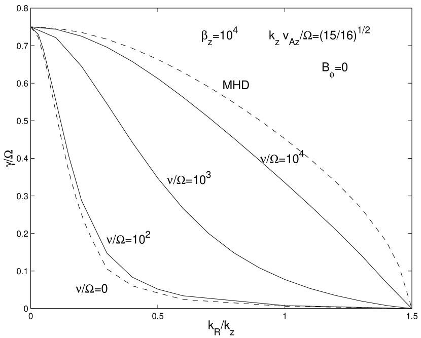
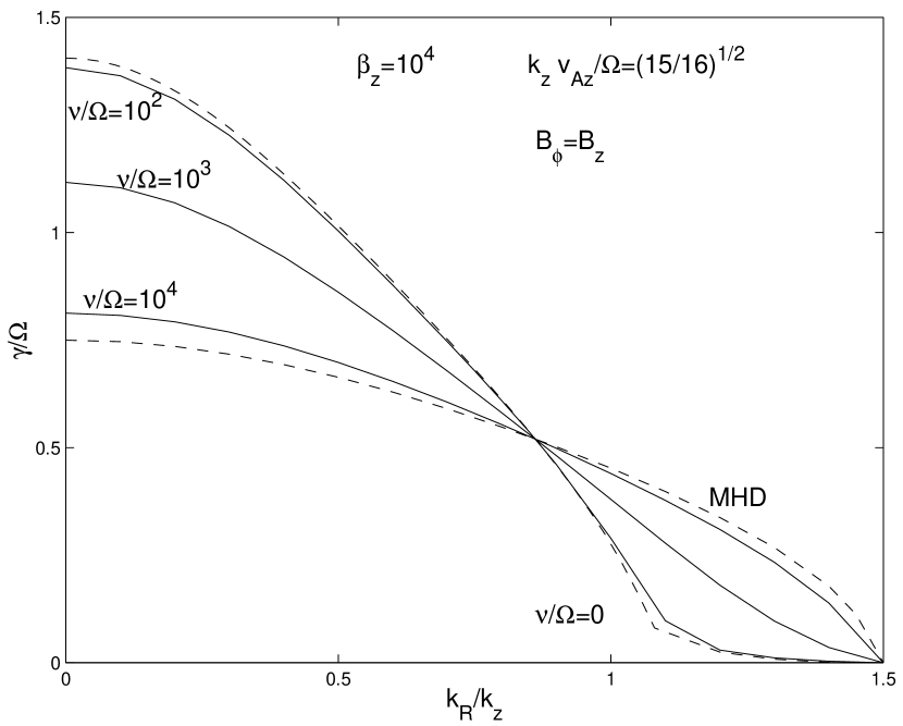
Figure 1: Growth rates of the MRI as a function of $k_{R}/k_{z}$ for different collision frequencies; $\beta_{z}=10^{4}$ and (a) $B_{\phi}=0$, (b) $B_{\phi}=B_{z}$. For $\nu/\Omega\geq 10^{4}$ the growth rates are very close to the MHD values, while for $\nu/\Omega\leq 10^{2}$ they are quite similar to the collisionless limit. The enhancement of the growth rate in the collisionless regime for small $k_{R}$ is the result of pressure anisotropy.

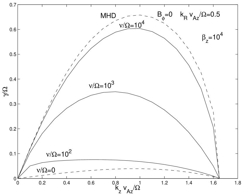
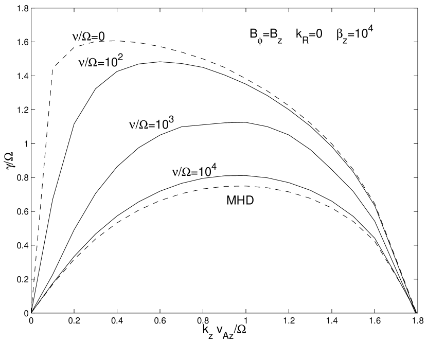
Figure 2: Growth rates of the MRI as a function of $k_{z}$ for different collisionalities.

Figures 1 and 2 show the growth rate of the MRI for intermediate values of collisionality in addition to the limits of zero and infinite (MHD) collision frequency (the latter two cases were shown in QDH). To produce these plots, we have used equations (7)-(11) and (33)-(36). These equations were solved both with a linear initial value code to find the fastest growing eigenmode, and with Mathematica to find the complete set of eigenvalues $\omega$.

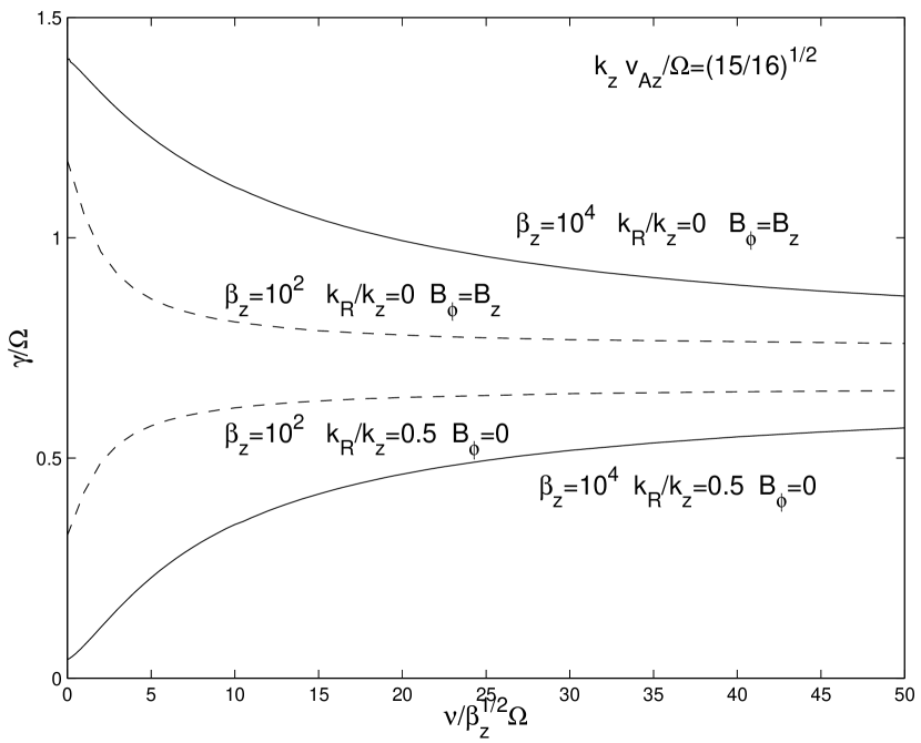
Figure 3: Variation of the MRI growth rate with collisionality for $k_{R}=0$, $B_{\phi}=B_{z}$ (top curves) and $k_{R}/k_{z}=0.5$, $B_{\phi}=0$ (bottom curves). Collisions isotropize the distribution function and can increase the growth rate in some regimes and decrease it in others. Continuous lines correspond to $\beta_{z}=10^{4}$ and dotted lines to $\beta_{z}=10^{2}$. The transition from collisionless to MHD regime takes place when $\nu/\Omega\approx\sqrt{\beta}$.

Figures 1 and 2 show that the transition from the MHD to the collisionless regime is fairly smooth and occurs, for these particular parameters, in the vicinity of $\nu/\Omega\sim 10^{3}$, which corresponds to $\nu\sim 10kc_{0}$, or $k\lambda_{mfp}\sim 0.1$, where $\lambda_{mfp}=c_{0}/\nu$ is the mean free path. Figure 3 shows the growth rate versus collisionality for $\beta_{z}=100$ and $\beta_{z}=10^{4}$, and for $B_{\phi}=B_{z}$, $k_{R}=0$ and $B_{\phi}=0$, $k_{R}/k_{z}=0.5$.

It is clear from these figures that the transition from the collisionless to the collisional MRI takes place at far higher collision rates than $\nu\sim\Omega\sim\omega$. That is, $\nu>\omega$ is not a sufficient criterion to be in the collisional regime. Instead, the collisional regime requires $\nu\gg|k_{\parallel}|c_{0}$, which can be written as $\nu/\Omega\gg\sqrt{\beta}|k_{\parallel}|v_{Az}/\Omega\approx\sqrt{\beta}$. Figure 3 shows that the much of the dependence on collisionality for different values of $\beta_{z}$ can be captured by plotting the growth rates vs. $\nu/\sqrt{\beta_{z}}\Omega$, though there is some residual variation.

At high $\beta\gg 1$, the Alfvén and MRI frequencies are small compared to the sound wave frequency, and there exists a regime $\omega\ll\nu\mathrel{\mathchoice{\vbox{\offinterlineskip\halign{$\m@th\displaystyle\hfil#\hfil$\cr<\crcr\sim\crcr} }}{\vbox{\offinterlineskip\halign{$\m@th\textstyle\hfil#\hfil$\cr<\crcr\sim\crcr} }}{\vbox{\offinterlineskip\halign{$\m@th\scriptstyle\hfil#\hfil$\cr<\crcr\sim\crcr} }}{\vbox{\offinterlineskip\halign{$\m@th\scriptscriptstyle\hfil#\hfil$\cr<\crcr\sim\crcr} }}}k_{\parallel}c_{0}$ where the collisionless results still hold despite the fact that the collision time is shorter than the growth rate of the mode. Physically, this is because in order to wipe out the pressure anisotropy that is crucial to the MRI in a collisionless plasma (see QDH) the collision frequency must be greater than the sound wave frequency, rather than the (much slower) growth rate of the mode. This can also be seen by comparing Figures 1 and 2 with the corresponding figures in QDH: the effect of increasing collisions (decreasing pressure anisotropy) is similar to that of decreasing $\beta_{z}$ (decreasing pressure force relative to magnetic forces). From the point of view of Snyder et al.’s fluid approach, the weak dependence of growth rate on collisionality even if $\nu$ is as large as $\omega$ can be understood from the fact that the terms proportional to $\omega$ and $\nu$ in equations (33) and (34) are both much smaller than the dominant terms involving convection, heat conduction, and magnetic forces. So the relative magnitudes of $\omega$ and $\nu$ are not that important, and it is not until $\nu$ is large enough to be relevant in equations (35)-(36) that collisional effects become noticeable.

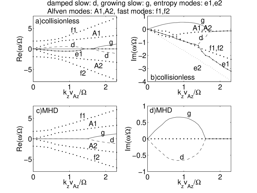
Figure 4: The real and imaginary parts of the mode frequency as a function of $k_{z}$ using collisionless Landau fluid closures (a,b) and MHD (c,d) are shown ($\nu=0$, $k_{R}v_{Az}/\Omega=0.5$, $\beta_{z}=10$, $B_{\phi}=0$).

Figure 4 shows the complete spectrum of eigenmode frequencies as $k_{z}$ is varied, including the propagating and damped modes in addition to the unstable MRI branch. We show all of the waves present in collisionless Landau fluid and MHD calculations for a fairly general choice of wavenumbers and a moderate $\beta_{z}=10$. The MRI is operational at lower $k_{z}$, while at high $k_{z}$ the eigenfrequencies eventually approach the uniform plasma limit.

Focusing first on the MHD solutions at high $k_{z}$, we see the standard set of 3 MHD waves: in order of descending frequency these are the fast magnetosonic wave, the shear Alfvén wave, and the slow wave. Equations (5)-(11) with an MHD adiabatic pressure equation $\omega\delta p=p_{0}{\bf k}\cdot\delta{\bf v}$ is a set of 8 equations with 8 eigenvalues for $\omega$. The standard 3 MHD waves provide 6 of the eigenvalues ($\pm\omega$ for oppositely propagating waves). The remaining roots are zero frequency modes (not shown in the plot). One is an entropy mode, corresponding to $\delta\rho/\rho_{0}=-\delta T/T_{0}$ so that $\delta p=0$. The other solution corresponds to an unphysical fluctuation that violates $\nabla\cdot{\bf B}=0$, which is eliminated by imposing the proper initial condition that $\nabla\cdot{\bf B}=0$. At lower $k_{z}$ in the MHD plots in Figure 4, it is the slow mode that is destabilized to become the MRI, as discussed in Balbus & Hawley (1998).

Turning next to the collisionless limit in Figure 4, there are two roots plotted in addition to the three “MHD-like” modes; this is because the single pressure equation of MHD is replaced by separate equations for the parallel and perpendicular pressure, so that there are now two entropy-like modes, both of which have non-zero frequencies but which are also strongly damped by collisionless heat conduction (which is neglected in MHD).

The fast, Alfvén, and slow waves in the collisionless calculation can again be identified in order of descending (real) frequency at high $k_{z}$. At lower $k_{z}$, one of the slow modes becomes destabilized to become the MRI, as in MHD. Unlike in MHD, however, the fast magnetosonic waves are strongly Landau damped since the resonance condition $\omega\sim k_{\parallel}c_{0}$ is easily satisfied. In addition, it is interesting to note that both the shear Alfvén and slow waves have some collisionless damping at the highest $k_{z}$ used in this plot, though the damping will approach zero for very high $k_{z}$. In a uniform plasma the shear Alfvén wave is undamped unless its wavelength is comparable to the proton Larmor radius or its frequency is comparable to the proton cyclotron frequency (neither of which is true for the modes considered here). By contrast, the slow mode is strongly damped unless $k_{\perp}\ll k_{\parallel}$ (e.g., Barnes 1966; Foote & Kulsrud 1979). The damping of small $k_{z}$ shear Alfvén waves in Figure 4 is due to the fact that our background plasma is rotating so the uniform-plasma modes are mixed together. Thus the well-known dissipation of the slow mode by transit-time damping also leads to damping of what we identify as the shear Alfvén wave (based on its high $k_{z}$ properties).

6 Summary and Discussion

In this paper we have extended the linear axisymmetric kinetic magnetorotational instability (MRI) calculation of QDH to include the effect of collisions. The MHD limit is recovered when the mean free path is short compared to the MRI wavelength, i.e., $\nu\gg k_{\parallel}c_{0}$, with a fairly smooth transition between the collisionless and collisional regimes. Interestingly the collisionless MRI results hold not only if $\nu\ll\omega$, but even when $\omega\ll\nu\ll k_{\parallel}c_{0}$. This intermediate regime can exist in $\beta\mathrel{\mathchoice{\vbox{\offinterlineskip\halign{$\m@th\displaystyle\hfil#\hfil$\cr>\crcr\sim\crcr} }}{\vbox{\offinterlineskip\halign{$\m@th\textstyle\hfil#\hfil$\cr>\crcr\sim\crcr} }}{\vbox{\offinterlineskip\halign{$\m@th\scriptstyle\hfil#\hfil$\cr>\crcr\sim\crcr} }}{\vbox{\offinterlineskip\halign{$\m@th\scriptscriptstyle\hfil#\hfil$\cr>\crcr\sim\crcr} }}}1$ plasmas because the MRI growth rate is slow compared to the sound wave frequency, $\omega\sim k_{\parallel}v_{A}=k_{\parallel}c_{0}\sqrt{2/\beta}\ll k_{\parallel}c_{0}$.

If we consider the application of our results to accretion flows, the collisionless limit will be applicable so long as $\nu/\Omega\mathrel{\mathchoice{\vbox{\offinterlineskip\halign{$\m@th\displaystyle\hfil#\hfil$\cr<\crcr\sim\crcr} }}{\vbox{\offinterlineskip\halign{$\m@th\textstyle\hfil#\hfil$\cr<\crcr\sim\crcr} }}{\vbox{\offinterlineskip\halign{$\m@th\scriptstyle\hfil#\hfil$\cr<\crcr\sim\crcr} }}{\vbox{\offinterlineskip\halign{$\m@th\scriptscriptstyle\hfil#\hfil$\cr<\crcr\sim\crcr} }}}\sqrt{\beta}$. This condition is amply satisfied for proton-proton and proton-electron collisions in all hot radiatively inefficient accretion flow models, suggesting that the collisionless limit is always appropriate. However, high frequency waves such as ion-cyclotron waves can isotropize the proton distribution function and thus provide an effective “collision” term crudely analogous to that considered here. It is difficult to estimate the importance of this process (e.g., whether its effective collision frequency is $\mathrel{\mathchoice{\vbox{\offinterlineskip\halign{$\m@th\displaystyle\hfil#\hfil$\cr>\crcr\sim\crcr} }}{\vbox{\offinterlineskip\halign{$\m@th\textstyle\hfil#\hfil$\cr>\crcr\sim\crcr} }}{\vbox{\offinterlineskip\halign{$\m@th\scriptstyle\hfil#\hfil$\cr>\crcr\sim\crcr} }}{\vbox{\offinterlineskip\halign{$\m@th\scriptscriptstyle\hfil#\hfil$\cr>\crcr\sim\crcr} }}}\Omega\sqrt{\beta}$) because we don’t know to what extent high frequency waves will be excited in the accretion flow. They are probably not significantly excited by the underlying MHD turbulence that drives accretion since this maintains low frequencies throughout the turbulent cascade (see Quataert’s 1998 discussion based on Goldreich & Sridhar 1995). High frequency waves may, however, be excited by shocks, reconnection events, or velocity space anisotropies.

One might anticipate that the linear differences between the collisionless and collisional MRI highlighted here and in QDH will imply differences in the nonlinear turbulent state in hot accretion flows (see, e.g., Hawley & Balbus 2002; Igumenshchev et al. 2003 for MHD simulations of such flows). Not only are there differences in the linear growth rates of the instability that drives turbulence, but the spectrum of damped modes is also very different. In particular, in the kinetic regime there exist modes at all scales in $|{\bf k}|$ that are subject to Landau/Barnes collisionless damping, while in the MHD regime the only sink for turbulent energy is due to viscosity/resistivity at very small scales (very high $|{\bf k}|$). Indeed, as we have shown, even long wavelength Alfvén waves can be damped by collisionless effects because of the mixture of uniform-plasma modes in the differentially rotating accretion flow (§5 and Fig. 4). Whether these differences are important or not may depend on how efficiently nonlinearities couple energy into the damped modes. These could modify the nonlinear saturated turbulent spectrum (e.g., the efficiency of angular momentum transport) or the fraction of electron vs. ion heating (the heating may also be anisotropic), which in turn determine the basic observational signatures of hot accretion flows (the accretion rate and the radiative efficiency). One approach for investigating nonlinear collisionless effects would be to extend existing MHD codes to include anisotropic pressure, the Snyder et al. (1997) fluid closure approximations for kinetic effects, and the BGK collision operator considered here. By varying the collision frequency, one can then scan from the collisionless kinetic to the collisional MHD regime, and assess any differences in the nonlinear turbulent state.

Appendix A Closure for high collisionality: $|\zeta|\gg 1$

For $|\zeta|\gg 1$, $Z\left(\zeta\right)\approx-1/\zeta-1/2\zeta^{3}-3/4\zeta^{5}$, $R\approx-1/2\zeta^{2}-3/4\zeta^{4}$, $1+2\zeta^{2}R\approx-3/2\zeta^{2}-15/4\zeta^{4}$, $Z-2\zeta R\approx 1/\zeta^{3}+3/\zeta^{5}$. Equation (26) then becomes

$$\frac{\delta n}{n_{0}}-\frac{\delta p_{\perp}}{p_{0}}=-\frac{\delta B}{B_{0}}\left(1+\frac{1}{2\zeta^{2}}\right)-\frac{\zeta_{2}}{\zeta}\left(1+\frac{1}{2\zeta^{2}}\right)\left(\frac{\delta T}{T_{0}}-\frac{\delta B}{B_{0}}\right).$$ (A1)

Assuming $|\zeta_{1}/\zeta_{2}|\ll 1$ (a high collisionality limit $\omega\ll\nu$) and using the binomial expansion we get

$$\frac{\delta n}{n_{0}}-\frac{\delta p_{\perp}}{p_{0}}=-\left\{1-\frac{\zeta_{1}}{\zeta_{2}}+\frac{1}{\zeta_{2}^{2}}\left(\frac{1}{2}+\zeta_{1}^{2}\right)-\frac{\zeta_{1}}{\zeta_{2}^{3}}\left(\frac{1}{2}+\zeta_{1}^{2}\right)\right\}\left(\frac{\zeta_{1}}{\zeta_{2}}\frac{\delta B}{B_{0}}+\frac{\delta T}{T_{0}}\right).$$ (A2)

To the lowest nonvanishing order one gets

$$\frac{\delta n}{n_{0}}\frac{\zeta_{1}}{\zeta_{2}}-\frac{\delta p_{\perp}}{p_{0}}\left(\frac{1}{3}+\frac{2}{3}\frac{\zeta_{1}}{\zeta_{2}}\right)+\frac{\delta p_{\parallel}}{p_{0}}\left(\frac{1}{3}-\frac{\zeta_{1}}{3\zeta_{2}}\right)=-\frac{\zeta_{1}}{\zeta_{2}}\frac{\delta B}{B_{0}}.$$ (A3)

Expanding equation (27) gives

$$-\frac{\delta n}{n_{0}}\left(\frac{3}{2\zeta^{2}}+\frac{15}{4\zeta^{4}}\right)+\frac{\delta p_{\parallel}}{p_{0}}\left(\frac{1}{2\zeta^{2}}+\frac{3}{4\zeta^{4}}\right)=-\frac{\delta B}{B_{0}}\left(\frac{1}{\zeta^{2}}+\frac{3}{\zeta^{4}}\right)$$

$$+\left(\frac{\delta B}{B_{0}}-\frac{\delta n}{n_{0}}+\frac{\delta T}{2T_{0}}\right)\zeta_{2}\left(\frac{1}{\zeta^{3}}+\frac{3}{\zeta^{5}}\right).$$ (A4)

Again using the binomial expansion for $|\zeta_{1}/\zeta_{2}|\ll 1$ we get

$$\frac{\delta n}{n_{0}}\left(-\frac{3}{2}\frac{\zeta_{1}}{\zeta_{2}}+\frac{9}{2}\left(\frac{\zeta_{1}}{\zeta_{2}}\right)^{2}+\frac{3}{4\zeta_{2}^{2}}\right)+\frac{\delta p_{\parallel}}{p_{0}}\left(\frac{1}{3}-\frac{1}{2}\frac{\zeta_{1}}{\zeta_{2}}+\frac{1}{2}\left(\frac{\zeta_{1}}{\zeta_{2}}\right)^{2}+\frac{1}{4\zeta_{2}^{2}}\right)$$

$$+\frac{\delta p_{\perp}}{p_{0}}\left(-\frac{1}{3}+\frac{\zeta_{1}}{\zeta_{2}}-2\left(\frac{\zeta_{1}}{\zeta_{2}}\right)^{2}-\frac{1}{\zeta_{2}^{2}}\right)=\frac{\delta B}{B_{0}}\left(-\frac{\zeta_{1}}{\zeta_{2}}+3\left(\frac{\zeta_{1}}{\zeta_{2}}\right)^{2}\right).$$ (A5)

The lowest order solution is

$$-\frac{3\zeta_{1}}{2\zeta_{2}}\frac{\delta n}{n_{0}}+\left(\frac{1}{3}-\frac{\zeta_{1}}{2\zeta_{2}}\right)\frac{\delta p_{\parallel}}{p_{0}}+\left(-\frac{1}{3}+\frac{\zeta_{1}}{\zeta_{2}}\right)\frac{\delta p_{\perp}}{p_{0}}=-\frac{\zeta_{1}}{\zeta_{2}}\frac{\delta B}{B_{0}}.$$ (A6)

We shall expand the parallel and perpendicular pressure perturbations as $\delta p_{\perp}=\delta^{0}p_{\perp}+\zeta_{1}/\zeta_{2}\delta^{1}p_{\perp}+(\zeta_{1}/\zeta_{2})^{2}\delta^{2}p_{\perp}+...$ and $\delta p_{\parallel}=\delta^{0}p_{\parallel}+\zeta_{1}/\zeta_{2}\delta^{1}p_{\parallel}+(\zeta_{1}/\zeta_{2})^{2}\delta^{2}p_{\parallel}+...$ From equations (A2) and (A5) one gets $\delta^{0}p_{\parallel}/p_{0}=\delta^{0}p_{\perp}/p_{0}=5\delta n/3n_{0}$ for the lowest order, and $(\delta p_{\perp}-\delta^{1}p_{\parallel})/p_{0}=3\delta B/B_{0}-2\delta n/n_{0}$. To the next order we can expand the solution as

$$\frac{\delta p_{\parallel}}{p_{0}}=\frac{5\delta n}{3n_{0}}+\frac{\zeta_{1}}{\zeta_{2}}\frac{\delta^{1}p_{\parallel}}{p_{0}}+\left(\frac{\zeta_{1}}{\zeta_{2}}\right)^{2}\frac{\delta^{2}p_{\parallel}}{p_{0}},$$ (A7)

$$\frac{\delta p_{\perp}}{p_{0}}=\frac{5\delta n}{3n_{0}}+\frac{\zeta_{1}}{\zeta_{2}}\left(\frac{\delta^{1}p_{\parallel}}{p_{0}}+3\frac{\delta B}{B_{0}}-2\frac{\delta n}{n_{0}}\right)+\left(\frac{\zeta_{1}}{\zeta_{2}}\right)^{2}\frac{\delta^{2}p_{\perp}}{p_{0}}.$$ (A8)

To the next order in $\zeta_{1}/\zeta_{2}$ in equation (A2) one gets

$$-\frac{1}{2\zeta_{1}^{2}}\frac{\delta n}{n_{0}}+\frac{1}{2}\frac{\delta^{1}p_{\parallel}}{p_{0}}+\frac{1}{3}\left(\frac{\delta^{2}p_{\parallel}}{p_{0}}-\frac{\delta^{2}p_{\perp}}{p_{0}}\right)=0.$$ (A9)

To the next order in equation (A5) we get

$$\left(2+\frac{1}{3\zeta_{1}^{2}}\right)\frac{\delta n}{n_{0}}-\frac{\delta^{1}p_{\parallel}}{p_{0}}+\frac{1}{3}\left(\frac{\delta^{2}p_{\parallel}}{p_{0}}-\frac{\delta^{2}p_{\perp}}{p_{0}}\right)=\frac{3\delta B}{B_{0}}.$$ (A10)

Equations (29) and (30) follow from equations (A9) and (A10).

Appendix B Closure for low collisionality: $|\zeta|\ll 1$

This regime is useful for low collisionality $\nu\ll k_{\parallel}c_{0}$ and high $\beta$, where the MRI is low frequency as compared to the sound wave frequency. Using the asymptotic expansion for $|\zeta|\ll 1$, $Z\left(\zeta\right)\approx i\sqrt{\pi}\left(1-\zeta^{2}\right)-2\zeta$ and $R\left(\zeta\right)\approx 1+i\sqrt{\pi}-2\zeta^{2}$, we simplify equation (26) to get

$$\frac{\delta n}{n_{0}}-\frac{\delta p_{\perp}}{p_{0}}=\frac{\delta B}{B_{0}}\zeta\left(i\sqrt{\pi}-2\zeta\right)+\left(\frac{\delta T}{T_{0}}-\frac{\delta B}{B_{0}}\right)\zeta_{2}\left(i\sqrt{\pi}-2\zeta\right).$$ (B1)

The lowest order term in $\zeta$ gives $\delta p_{\perp}/p_{0}=\delta n/n_{0}$. Let $\delta p_{\perp}/p_{0}\approx\delta n/n_{0}+\zeta\delta^{1}p_{\perp}/p_{0}$. To the next order one gets

$$\zeta\frac{\delta^{1}p_{\perp}}{p_{0}}=-i\sqrt{\pi}\zeta\frac{\delta B}{B_{0}}+i\sqrt{\pi}\zeta_{2}\frac{\delta B}{B_{0}}=-i\sqrt{\pi}\zeta_{1}\frac{\delta B}{B_{0}}.$$ (B2)

Therefore to second order in $\zeta$, $\delta p_{\perp}/p_{0}\approx\delta n/n_{0}-i\sqrt{\pi}\zeta_{1}\delta B/B_{0}+\zeta^{2}\delta^{2}p_{\perp}/p_{o}$. On using the asymptotic formula for $Z$ and $R$ in equation (27), one gets

$$\frac{\delta n}{n_{0}}-\left(1+i\sqrt{\pi}\zeta\right)\frac{\delta p_{\parallel}}{p_{0}}=-i\sqrt{\pi}\zeta\frac{\delta B}{B_{0}}-\zeta_{2}\left(i\sqrt{\pi}-4\zeta\right)\left(\frac{\delta n}{n_{0}}-\frac{\delta T_{\parallel}}{2T_{0}}-\frac{\delta B}{B_{0}}\right).$$ (B3)

To the lowest order one gets $\delta p_{\parallel}/{p_{0}}={\delta n}/{n_{0}}$, so let ${\delta p_{\parallel}}/{p_{0}}\approx{\delta n}/{n_{0}}+\zeta{\delta^{1}p_{\parallel}}/{p_{0}}$. To the next order,

$$\zeta\frac{\delta^{1}p_{\parallel}}{p_{0}}=-i\sqrt{\pi}\zeta_{1}\frac{\delta n}{n_{0}}+i\sqrt{\pi}\zeta_{1}\frac{\delta B}{B_{0}}.$$ (B4)

Therefore through second order $\delta p_{\parallel}/p_{0}\approx\delta n/n_{0}+i\sqrt{\pi}\zeta_{1}\left(\delta B/B_{0}-\delta n/n_{0}\right)+\zeta^{2}\delta^{2}p_{\parallel}/p_{0}$. The comparison of the terms of the order $\zeta^{2}$ in equation (26) give

$$\zeta^{2}\frac{\delta^{2}p_{\perp}}{p_{0}}=2\zeta_{1}\zeta\frac{\delta B}{B_{0}}-\frac{\pi}{3}\zeta_{1}\zeta_{2}\left(\frac{\delta B}{B_{0}}+\frac{\delta n}{n_{0}}\right),$$ (B5)

and the terms of the order $\zeta^{2}$ in equation (27) give

$$\zeta^{2}\frac{\delta^{2}p_{\parallel}}{p_{0}}=\left(4\zeta_{1}\zeta_{2}-\pi\zeta_{1}^{2}-\frac{7\pi}{6}\zeta_{1}\zeta_{2}\right)\frac{\delta n}{n_{0}}+\left(\sqrt{\pi}\zeta_{1}\zeta-\frac{\pi}{6}\zeta_{1}\zeta_{2}-2\zeta^{2}-4\zeta_{2}\zeta\right)\frac{\delta B}{B_{0}}.$$ (B6)

From equations (B5) and (B6) the asymptotic expansion in equations (31) and (32) follow.

References

• Balbus & Hawley (1991) Balbus, S. A. $\&$ Hawley, J. F. 1991, ApJ, 376, 214
• Balbus & Hawley (1998) Balbus, S. A. $\&$ Hawley, J. F. 1998, Rev. Mod. Phys., 70, 1
• Barnes (1966) Barnes. A. 1966, Phys. Fluids 9, 1483
• Bhatnagar, Gross, & Krook (1954) Bhatnagar, P. L., Gross, E. P. $\&$ Krook, M., 1954, Phy. Rev., 94, 511
• Chew, Goldberger, & Low (1956) Chew, G. F., Goldberger, M. L. $\&$ Low, F. E., 1956, Proc. R. Soc. London, Ser. A, 236, 112
• Dimits et al. (2000) Dimits, A. M., Bateman, G., Beer, M. A., Cohen, B. I., Dorland, W., Hammett, G. W., Kim, C., Kinsey, J. E., Kotschenreuther, M., Kritz, A. H., Lao, L. L., Mandrekas, J., Nevins, W. M., Parker, S. E., Redd, A. J., Shumaker, D. E., Sydora, R., Weiland, J., 2000, Phys. Plasmas 7, 969
• Esin et al. (1997) Esin, A., McClintock, J. E. & Narayan R., 1997, ApJ, 489, 865
• Foote & Kulsrud (1979) Foote, E. A. $\&$ Kulsrud, R. M., 1979, ApJ, 233, 302
• Goldreich & Sridhar (1995) Goldreich, P. & Sridhar, S. 1995, ApJ, 438, 763
• Hammett et al. (1993) Hammett, G. W., Beer, M. A., Dorland, W., Cowley, S. C. & Smith, S. A., 1993, Plasma Phys. Control. Fusion , Vol. 35, 973
• Hammett et al. (1992) Hammett, G. W., Dorland, W. & Perkins, F.W., 2002, Phys. Fluids B4, 2052
• Hawley & Balbus (2002) Hawley, J. F. & Balbus, S. A., 2002, ApJ, 573, 738
• NRL Formulary (2000) Huba, J. D., 2000, “NRL Plasma Formulary”, (Naval Research Laboratory, Washington, DC), 30
• Igumenshchev et al. (2003) Igumenshchev, I. V., Abramowicz, M. A. & Narayan, R., 2003, ApJ submitted (astro-ph/0301402)
• Kruskal & Oberman (1958) Kruskal, M. D. $\&$ Oberman, C. R. 1958, Phys. Fluids 1, 275
• Kulsrud (1983) Kulsrud, R. M., 1983, in “Handbook of Plasma Physics”, ed. M. N. Rosenbluth $\&$ R. Z. Sagdeev (North Holland, New York)
• Mattor (1992) Mattor N 1992, Phys. Fluids B 4, 3952
• Parker et al. (1994) Parker, S. E., Dorland, W., Santoro, R. A., Beer, M. A., Liu, Q. P., Lee, W. W., & Hammett, G. W., 1994, Phys. Plasmas, 1, 1461
• Quataert (1998) Quataert, E., 1998, ApJ, 500, 978
• Quataert (2003) Quataert, E., 2003, to be published in Astron. Nachr., Vol. 324, No. S1 (2003), Special Supplement “The central 300 parsecs of the Milky Way”, Eds. A. Cotera, H. Falcke, T. R. Geballe, S. Markoff
• Quataert et al. (2002) Quataert, E. J., Dorland, W., $\&$ Hammett, G. W., 2002, ApJ, 577, 524
• Rosenbluth & Rostoker (1959) Rosenbluth, M. D., & Rostoker, N. 1959, Phys. Fluids 2, 23
• Smith (1997) Smith, S. A., 1997, Princeton University Ph.D. Thesis, “Dissipative Closures for Statistical Moments, Fluid Moments, & Subgrid Scales in Plasma Turbulence” To be posted at www.arxiv.org.
• Snyder et al. (1997) Snyder, P. B., Hammett, G. W., $\&$ Dorland, W., 1997, Phys. Plasmas 4, 3974