Cosmology with the Ly-$\alpha$ forest

Abstract

The Ly$\alpha\$forest has emerged as one of the few systems capable of probing small-scale structure at high-$z$ with high precision. In this talk I highlight two areas in which the Ly$\alpha\$forest is shedding light on fundamental questions in cosmology, one speculative and one which should be possible in the near future.

I Introduction

As we heard in the talks by Uros Seljak and Lam Hui in this meeting, the physics of the Ly$\alpha\$forest, as measured in high-$z$ Quasi-Stellar Object (QSO) spectra, is reasonably simple. At these redshifts the gas making up the intergalactic medium is in photoionization equilibrium, which results in a tight density–temperature relation for the absorbing material with the neutral hydrogen density proportional to a power of the baryon density. Since pressure forces are sub-dominant, the neutral hydrogen density closely traces the total matter density on the scales relevant to the forest ($0.1-10\,h^{-1}$Mpc). The structure in QSO absorption thus traces, in a calculable way, slight fluctuations in the matter density of the universe back along the line of sight to the QSO, with most of the Ly$\alpha\$forest arising from over-densities of a few times the mean density.

In this contribution I want to focus on two areas where the Ly$\alpha\$forest can be used to constrain cosmology and astrophysics. The first, dealing with measuring the matter power spectrum at high redshift, is quite speculative, but might be very exciting. The second has a higher chance of success and may tell us something about the nature of the ionizing sources, the end of the dark ages and the formation of the first objects in the universe.

II Finding baryons at $z>1$?

The presence of a series of almost regularly spaced peaks in the cosmic microwave background temperature angular power spectrum has now been compellingly demonstrated. The same physics which gives rise to these peaks, acoustic oscillations in the baryon-photon plasma prior to recombination PeeYu , also predicts a (much smaller) series of peaks in the matter power spectrum. A measurement of these peaks would provide a fundamental test of the paradigm, and an independent measure of the $z$-dependent Hubble constant and distance-redshift relation EisHuSilSza ; EisHuTeg ; MeiWhiPea ; Eisenstein ; BlaGla ; Lin . Because non-linear growth ‘washes out’ the peaks MeiWhiPea they are best searched for at high redshift.

The baryon oscillations themselves lie at $k\simeq 0.03-0.3\,h/$Mpc (see Fig. 1), with an amplitude of 5% or less for currently popular cosmological models EisHuSilSza ; MeiWhiPea . The higher modes are roughly out of phase with the photon peaks (also in $k$-space) and appear half as often as the peaks in the CMB spectrum (see e.g. Fig. 1 of MeiWhiPea ). The peaks are suppressed by Silk damping beyond $k\sim 1\,h/$Mpc.

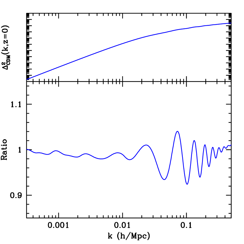
Figure 1: The contribution to the dark matter variance per $\log k$, $\Delta^{2}(k)$, in linear theory. The upper panel shows $\Delta^{2}(k)$ on a logarithmic scale while the lower panel shows the ratio of the numerically computed $\Delta^{2}(k)$ WhiSco to the fitting function of EisHu with the oscillations suppressed.

Naively the best way to measure the small baryonic oscillations in the matter power spectrum would be an ultra-large galaxy redshift survey at high-$z$. Such a survey would require next-generation instruments and a large dedicated team. Thus even with adequate funding and heroic efforts it is several years away. It is therefore interesting to explore whether one could measure the baryonic oscillations another way.

Within a few years the SDSS will return a catalogue of $\sim 10^{5}$ QSOs over $\sim 10^{4}$ square degrees of sky. These quasars will be distributed in both redshift and angular separation, but simple counting suggests that one should find many hundreds to several thousands with separations of tens of Mpc above $z\sim 2$. It is therefore interesting to ask whether this sample could be used to probe the baryon oscillations.

Using simply the auto-power spectrum of the forest will not work, because the line-of-sight spectrum at $k$ is an integral of the 3D spectrum over wavenumbers greater than $k$. This integration suppresses the small oscillations which are our primary signal. However one can consider the cross-spectra, where one line-of-sight is cross-correlated with a neighboring line-of-sight. As we shall show below this statistic is sensitive to the oscillations. In addition uncorrelated errors from e.g. continuum fitting, should be averaged down in this procedure relative to their value in the auto-spectrum. Since we are working on large scales, where the noise is essentially absent, one could in principle measure the flux cross-spectrum to the cosmic variance limit

$${\delta\pi_{\tau}\over\pi_{\tau}}\simeq\sqrt{2k_{f}\over N\Delta k}$$ (1)

where $N$ is the number of pairs, $k_{f}$ is the fundamental mode along the line-of-sight and $\Delta k$ is the width of the bin in $k$-space in which we are measuring the power. We can alternatively write $k_{f}=2\pi/L$, where $L$ is the length of the ‘useful’ part of the spectrum. Unless we attempt to fit to the higher lines, the useful length of the spectrum is the section between Ly$\alpha\$and Ly$\beta$ which covers hundreds of Mpc in the rest frame of the absorbers. Thus with a few hundred pairs it is possible to measure the cross-spectrum with error bars on the order of per cent.

One major advantage here is that, like the CMB itself, the redshift and scale dependence of the peaks is accurately calculable given a cosmological model. This allows us to perform a likelihood estimation of the relevant cosmological factors, including pairs of different distances and redshifts, rather than attempt to perform an inversion on the irregularly sampled data. Though the latter can be done, it is considerably more difficult than the ‘forward’ approach.

By applying the idea of the peak-background split from large-scale structure is it possible to show that, for sufficiently large scales and assuming $\tau=A(\rho/\bar{\rho})^{\alpha}$, the flux cross-spectrum, $\pi_{\tau}$, along two lines of sight separated by distance $x_{\perp}$ is proportional to the dark matter cross-power spectrum $\pi$ (see also McDonald ; Viel ). On these very large scales we can neglect the effects of thermal broadening or peculiar velocities. The DM cross-spectrum is simply related to the 3D power spectrum by

$$\pi^{2}(k,x_{\perp})=\int_{k}^{\infty}{dq\over q}\left({k\over q}\right)J_{0}(\sqrt{q^{2}-k^{2}})\Delta^{2}(q)$$ (2)

or Viel

$$\Delta^{2}(q)=\int_{0}^{\infty}{dx\over x}\left({qx}\right)^{2}J_{0}(x\sqrt{q^{2}-k^{2}})\pi^{2}(q)$$ (3)

where the inverse relation holds $\forall\ k<q$. Note that for smooth spectra, $\pi^{2}(k)$ gets contributions from $k<q<x_{\perp}^{-1}$. As $x_{\perp}\to 0$, $J_{0}\to 1$ and we find the auto-spectrum is the projection of the 3D spectrum as anticipated.

Converting from $h/$Mpc to s/km using $H(z)=H_{0}\sqrt{\Omega_{M}(1+z)^{3}+\Omega_{\Lambda}}\sim 100\,{\rm km}/{\rm s}/{\rm Mpc}$ we find that the relevant spectral range is roughly $3\times 10^{-4}$s/km to $3\times 10^{-3}$s/km. This is quite large scale, roughly comparable to the fundamental mode if we measure only from 100nm to 120nm.

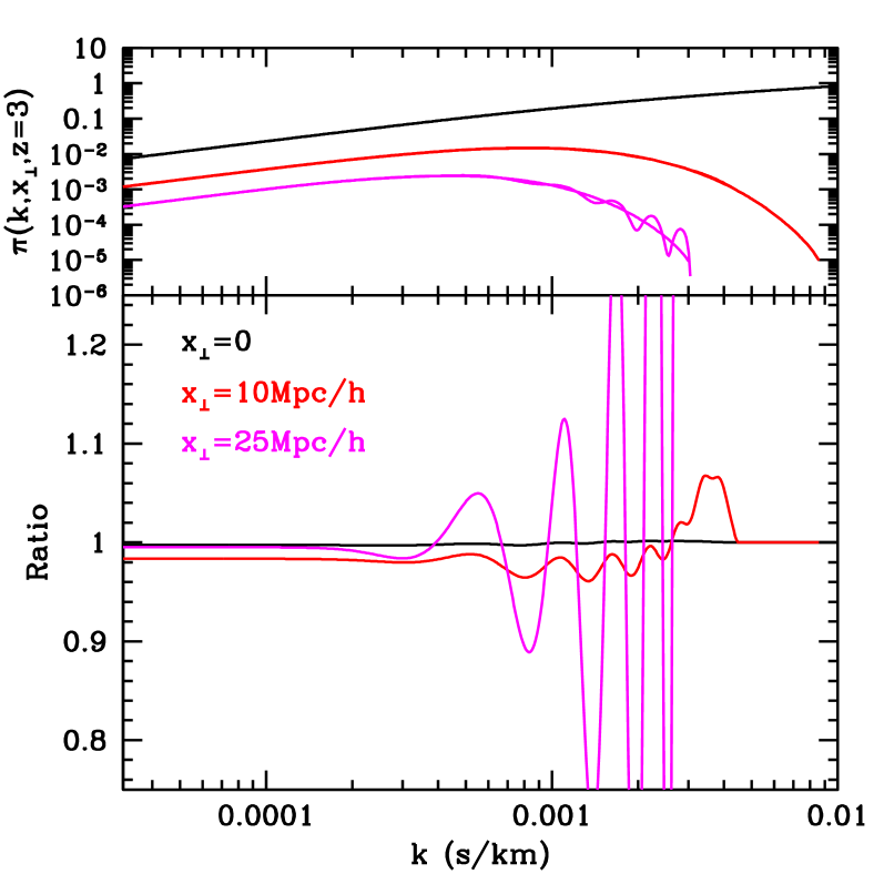
Figure 2: The cross-power spectra of the DM, in linear theory, at $z=3$. The upper panel shows $\pi(k,x_{\perp})$, including and excluding the baryonic oscillations, for different values of $x_{\perp}$. The lower panel shows the ratio to the smooth fitting function of EisHu .

On the positive side Fig. 2 shows that the signal is present in the cross spectra at separations of 10Mpc or so. The relative amplitude of the oscillations (which is the figure of merit for cosmic variance dominated measurements) can be quite large, 10% or more, compared to the accuracy with which $\pi$ can be measured. Because we can accurately predict the positions and amplitudes of the peaks we know both the $x_{\perp}$ and $z$ dependence of the signal.

On the negative side there is only a small fractional change in $\pi$ when $\pi$ is big (i.e. $x_{\perp}$ small) and the larger fractional change in $\pi$ when $\pi$ is small. This suggests we would be working primarily at very low signal levels, where systematics become increasingly important. Also, if we work with the spectra only between Ly$\alpha\$and Ly$\beta$ we do not have very much ‘spare’ resolution in $k$ to see the oscillations. We would ideally probe $k\ll 0.003$s/km which requires very long spectra.

In summary, the signal of baryon oscillations is lurking in the cross-spectra of QSO pairs, which allow us to probe large volumes of space at high redshift with a modest investment in telescope time. A naive estimate of the cosmic variance limitations of a QSO survey like the SDSS suggests that the signal could be seen in a likelihood analysis with high confidence. However the overall signal levels are very low and there are numerous sources of systematic error which may make the signal forever unmeasurable.

III The nature of the ionizing sources

Currently the sources that make up the UV background are unknown. However the mean optical depth $\bar{\tau}$ in the Ly$\alpha\$forest offers a way to constrain the source emissivity and fluctuations in the UVbg can be used to constrain the nature of the sources. I have been involved in a long-running collaboration with Avery Meiksin to investigate these issues PaperI ; PaperII , and present some of our basic results here.

First we consider the constraints on the source emissivity $\epsilon$. Given a cosmological model, the mean flux or optical depth $\bar{\tau}$ fixes the ionization rate $\Gamma$. If we approximate $\exp[-\tau]$ as $\exp[-\ell/r_{0}]$ where $r_{0}$ is the attenuation length then $\Gamma\sim\epsilon r_{\rm eff}$. Here $r_{\rm eff}$ is an effective attenuation length which interpolates between the attenuation limited ($r_{0}\ll\ell_{H}$) and cosmological expansion+age limited ($r_{0}\gg\ell_{H}$) regimes and $\ell_{H}$ is the Hubble distance.

As a function of $\epsilon$ the transition between the attenuation limited and cosmologically limited regimes is very abrupt, and at fixed $\epsilon$, $r_{0}$ falls rapidly with increasing redshift. This in turn means that $\bar{\tau}$ rises rapidly, almost exponentially, with redshift.

Figure 3: (Upper) The emissivity, at the Lyman edge, required to fit the mean flux observed in QSO spectra as a function of wavelength (points) compared to extrapolated QSO emissivities for 3 different assumptions about the evolution of the QSO luminosity function (lines). Under these assumptions QSOs would be enough to keep the universe ionized at $z\leq 6$. (Lower) The attenuation length, $r_{0}$ in proper Mpc/$h$, as a function of $z$. Note that $r_{0}$ drops quasi-exponentially to $z\sim 6$.

Fig. 3 shows the emissivity of the sources, as a function of $z$, required to fit the observed $\bar{\tau}$. This is compared to extrapolations of the QSO luminosity function. From this we can see that QSOs may contribute a substantial fraction of the UV background even as high as $z\sim 6$. If QSOs do contribute non-negligibly to the UV background then we would expect large spatial fluctuations in $\Gamma$. Conversely, if galaxies or star clusters dominate the UV background we expect to see only the imprint of large-scale structure. Unfortunately the effects of UV background correlations are most conspicuous at $z>5$, where the precise level of absorption by the Ly$\alpha\$forest is most difficult to measure because of extremely low flux values.

Figure 4: (Upper) The normalized flux, as a function of velocity, from a PM simulation of structure formation. The spectra were computed as described in PaperI ; PaperII assuming either a uniform ionizing background (dashed) or that the background was dominated by a single source at the center of the box (dotted). (Lower) The dark matter density (dotted) along the line-of-sight or the inverse ionization rate, $\Gamma^{-1}$, in units of the average (dashed).

Fig. 4 shows how a simulated Ly$\alpha\$spectrum is changed if the UV background is (unrealistically) dominated by a single source as compared to the usually assumed smooth behavior. To assess a more realistic situation it is necessary to resort to Monte Carlo simulations in which sources are placed within the simulation volume, the UV background computed and then spectra created from the density and velocity fields within the box. Our investigations suggest that the 1-point distribution is relatively unaffected by fluctuations in the UVbg, however the 2-point statistics (the flux correlation function and power spectrum) show noticeable differences at high redshift PaperII . In addition fluctuations in the UVbg will increase the estimated Ly$\alpha\$optical depth over the value that would be estimated assuming a homogeneous background PaperI . This increases the demand placed on the ionization rate required to reproduce $\bar{\tau}$ and needs to be included when comparing with estimates of source emissivity.

IV Conclusions

The Ly$\alpha\$forest is emerging as a powerful probe of structure formation at high redshift. Because the physics is relatively well understood we can compare increasingly realistic calculations with ever better data to constrain our cosmological models. Here we have investigated two ways in which the Ly$\alpha\$forest constrains cosmology. The first, speculative, proposal was to search for baryonic oscillations in the matter power spectrum through their imprint in the Ly$\alpha\$forest cross-spectra. The second proposal was to constrain the emissivity of the sources of the UV background using the measured mean optical depth of QSO spectra.

In the first case we found that while in principle the signal-to-noise and statistics of the signal were favorable, in practice the very low signal levels made this measurement prone to numerous systematic effects. In the second case we showed that reasonable extrapolations of the QSO luminosity function to high-$z$ would allow QSOs to contribute a non-negligible fraction of the UV background even as early as $z=6$. If this turns out to be the case, the UV background should have relatively large spatial fluctuations which can affect the 2-point statistics of the forest at high $z$.

Acknowledgements: I thank Simon White for allowing me to present our work on baryon oscillations in the Ly$\alpha\$forest, and Avery Meiksin for several years of productive collaborations, including many enlightening conversations on the physics of the IGM. I would also like to thank the organizers for such an interesting and successful conference.

References

- (1) P.J.E. Peebles, J.T. Yu, ApJ, 162, 815 (1970).
- (2) D. Eisenstein, W. Hu, M. Tegmark, ApJ, 504, L57 (1999).
- (3) see e.g. D. Eisenstein (2003) [astro-ph/0301623]
- (4) D. Eisenstein, W. Hu, J. Silk, A.S. Szalay, ApJ, 494, L1 (1998).
- (5) A. Meiksin, M. White, J.A. Peacock, MNRAS 304, 851 (1999) [astro-ph/9812214]
- (6) C. Blake, K. Glazebrook, preprint [astro-ph/0301632]
- (7) E.V. Linder, preprint [astro-ph/0304001]
- (8) M. White, D. Scott, ApJ, 459, 415 (1996).
- (9) P. McDonald, et al., ApJ, 543, 1 (2000) [Appendix C]
- (10) M. Viel, S. Matarrese, H.J. Mo, M.G. Haehnelt, T. Theuns, MNRAS, in press, [astro-ph/0105233]
- (11) D. Eisenstein, W. Hu, ApJ, 511, 5 (1999).
- (12) A. Meiksin, M. White, MNRAS, in press [astro-ph/0303302]
- (13) A. Meiksin, M. White, MNRAS, submitted