Detecting Reflected Light from Close-In Extrasolar Giant Planets with the Kepler Photometer

Abstract

NASA’s Kepler Mission promises to detect transiting Earth-sized planets in the habitable zones of solar-like stars. In addition, it will be poised to detect the reflected light component from close-in extrasolar giant planets (CEGPs) similar to 51 Peg b. Here we use the DIARAD/SOHO time series along with models for the reflected light signatures of CEGPs to evaluate Kepler’s ability to detect such planets. We examine the detectability as a function of stellar brightness, stellar rotation period, planetary orbital inclination angle, and planetary orbital period, and then estimate the total number of CEGPs that Kepler will detect over its four year mission. The analysis shows that intrinsic stellar variability of solar-like stars is a major obstacle to detecting the reflected light from CEGPs. Monte Carlo trials are used to estimate the detection threshold required to limit the total number of expected false alarms to no more than one for a survey of 100,000 stellar light curves. Kepler will likely detect 100-760 51 Peg b-like planets by reflected light with orbital periods up to 7 days.

1 Introduction

The discovery of 51 Peg b by Mayor & Queloz et al. (1995) ignited a firestorm in the astronomical community. Eight years later, over 100 extrasolar planets have been found, including multiple planet systems (Butler et al., 1999), and planets in binary systems (Cochran et al., 1997). The quest for extrasolar giant planets has moved beyond the question of detecting them to the problem of studying their atmospheres. Shortly after the seminal discovery of 51 Peg b, attempts were made to detect spectroscopically the light reflected from extrasolar planets in short-period orbits (Cameron et al., 1999; Charbonneau et al., 1999). To date, no solid detection of the reflected light component has been reported for any extrasolar planet, although Charbonneau et al. (2002) report the detection of a drop in the sodium line intensity from the atmosphere of HD209458b during a transit of its parent star.

The lack of a reflected light component detection is puzzling since a planet exhibiting a Lambert-like phase function with an albedo similar to that of Jupiter should be detectable. The work of Seager et al. (2000) provides a possible reason for the lack of detections: realistic model atmospheres could be significantly less reflective than would be expected from a Lambert sphere. Efforts to detect the periodic reflected light components of CEGPs might be forced to wait for the first generation of space-based photometers, of which several are scheduled to be launched in the near future.

The Canadian MOST, the Danish MONS (Perryman, 2000), and the CNES mission COROT (Schneider et al., 1998) all promise to study the miniscule photometric variations indicative of acoustic oscillations in nearby stars, effectively peering within their hearts to reveal their internal structure. These missions will be able to study the intrinsic stellar variations of the stars they target, much as the p-modes of the Sun have been studied by ESA’s SOHO Mission (Fröhlich et al., 1997). If the stellar variability does not prove insurmountable, some of these missions may well be able to detect the reflected light components of the previously discovered CEGPs. In general, the time spent on each target star will not allow these missions to discover new planets this way, although COROT has the best chances of doing so, as it surveys a field of stars for several months at a time, rather than observing a single star at a time. There are, however, larger, more ambitious photometric missions on the horizon. Both NASA’s Kepler Mission and ESA’s Eddington Mission will be launched in 2007 to search for Earth-sized planets transiting solar-like stars. The exquisite photometric precision promised by these two missions (better than $2\times 10^{-5}$ on timescales of $\sim$1 day) will not only allow for discovery of transiting planets and stunning asteroseismology, but might also produce a significant number of detections of the reflected light from CEGPs.

The reflected light signature of an extrasolar planet appears uncomplicated at first, much like the progression of the phases of the moon. As the planet swings along its orbit towards opposition, more of its star-lit face is revealed, increasing its brightness. Once past opposition, the planet slowly veils her lighted countenance, decreasing the amount of light reflected toward an observer. As the fraction of the visible lighted hemisphere varies, the total flux from the planet-star system oscillates with a period equal to the planetary orbital period. Seager et al. (2000) showed that the shape of the reflected light curve is sensitive to the assumed composition and size of the condensates in the atmosphere of a CEGP. While this presents an opportunity to learn more about the properties of an atmosphere once it is discovered, it makes the process of discovery more complex: The reflected light signatures are not as readily characterized as those of planetary transits, so that an ideal matched filter approach does not appear viable. The signatures from CEGPs are small ($<$100 ppm) compared to the illumination from their stars, requiring many cycles of observation to permit their discovery. This process is complicated by the presence of stellar variability which imposes its own variations on the mean flux from the star. Older, slowly rotating stars represent the best targets. They are not as active as their younger counterparts, which are prone to outbursts and rapid changes in flux as star spots appear, evolve and cross their faces. In spite of these difficulties, a periodogram-based approach permits the characterization of the detectability of CEGPs from their reflected light component.

Our study of this problem began in 1996 in support of the proposed Kepler Mission to the NASA Discovery Program (Borucki et al., 1996; Doyle, 1996). That study used measurements of solar irradiance by the Active Cavity Radiometer for Irradiance Monitoring (ACRIM) radiometer aboard the Solar Maximum Mission (SMM) (Willson & Hudson, 1991), along with a model for the reflected light signature based on a Lambert sphere and the albedo of Jupiter. Here we significantly extend and update the previous preliminary study using measurements by the Dual Irradiance Absolute Radiometer (DIARAD), an active cavity radiometer aboard the Solar Heliospheric Observatory (SOHO) (Fröhlich et al., 1997) along with models of light curves for 51 Peg b–like planets developed by Seager et al. (2000). For completeness, we include Lambert sphere models of two significantly different geometric albedos, $p$=0.15 and $p$=2/3. The SOHO data are relatively complete, extend over a period of 5.2 years, are evenly sampled at 3 minutes, a rate comparable to that for Kepler’s photometry (15 minutes), and have the lowest instrumental noise of any comparable measurement of solar irradiance. Seager et al. (2000) provide an excellent paper describing reflected light curves of CEGPs in the visible portion of the spectrum. However, they do not consider the problem of detecting CEGP signatures in realistic noise appropriate to high precision, space-based photometers.

The current article complements our study of the impact of solar-like variability on the detectability of transiting terrestrial planets for Kepler (Jenkins, 2002). The observational noise encountered in the detection of transiting small planets and in the detection of the reflected light component of CEGPs is the same: only the shape, timescale and amplitude of the signal of interest have changed. We have also conducted a more thorough analysis of the false alarm rates and the requisite detection thresholds than that performed in our preliminary study and have developed a detection scheme to accommodate the non-sinusoidal nature of the reflected light curves produced by CEGPs. In this paper, our focus is on the Kepler Mission due to our familiarity with its design parameters and its expected instrumental noise component, although the results should apply to other missions with similar apertures, instrumental noise, and mission durations.

In this study, we analyze different combinations of model planetary atmospheres, stellar rotation periods, and stellar apparent magnitudes, examining the detectability of each case over a range of orbital inclinations, $I$, from edge–on ($I=90^{\circ}$) to near broadside ($I=10^{\circ}$), and over orbital periods, $T_{p}$, from 2 to 7 days. The brightnesses considered for the stars range from $m_{R}$=9.0 to $m_{R}$=15.0, which dictate the corresponding shot and instrument noise for the Kepler target stars. To simulate the reflected component of the light curve we use two atmospheric models developed by Seager et al. (2000): one for clouds with a mean particle radius, $\bar{r}$, of 0.1 $\mu$m consisting of a mixture of Fe, MgSiO₃, and Al₂O₃, and the same mixture, but for clouds with $\bar{r}=1.0$ $\mu$m. We also consider two Lambert sphere models, one with maximum reflectivity, and one with a geometric albedo of 0.15 (corresponding to the case of Mars). Different models of stellar variability are considered, all based on the DIARAD/SOHO time series, which were resampled and scaled to obtain synthetic light curves for stars with rotation periods between 5 and 40 days as per Jenkins (2002). For each set of parameters, a periodogram analysis yields the expected detection statistic for a 1.2 Jupiter radius (R_J) planet. The appropriate detection thresholds and resulting detection rates are determined from Monte Carlo runs using the same detection procedure applied to White Gaussian Noise (WGN) sequences. The resulting detection rates are averaged over all orbital inclinations and over the expected distribution of CEGP orbital periods, and are then used in conjunction with a model distribution of main sequence stars in Kepler’s field of view (FOV) to estimate the total number of CEGPs detected by reflected light. The results indicate that Kepler should detect 100-760 CEGPs in orbits up to 7 days in period around old, quie, solar-like stars. These detections will not occur in the first weeks of the mission due to the low amplitudes of the planetary signatures. Rather, they will accumulate steadily over the course of the mission.

The paper is organized as follows: We present the DIARAD/SOHO measurements of solar variability in §2, followed by a discussion of Seager et al. (2000)’s light curve models for the reflected light component from CEGPs in §3. A summary of the Kepler Mission is given in §4. Section §5 describes the galactic model for the distribution of Kepler’s target stars used to optimize the proposed detection algorithm and analyze its performance. Our approach to detecting strictly periodic signals in noise and setting detection thresholds and assessing detection rates is given in §6. Monte Carlo experiments conducted to establish false alarm rates and the requisite detection thresholds are discussed in §7. The expected number of detections is presented in §8. A discussion of sources of confusion and methods to reject false positives is given in §9. We conclude in §10 by summarizing the findings and giving suggestions for future work.

2 The DIARAD/SOHO Observations

In order to study the capabilities of missions such as Kepler, we take measurements from the DIARAD instrument aboard the SOHO spacecraft as a proxy for all solar-like stars. DIARAD is a redundant, active-cavity radiometer aboard SOHO that measures the white-light irradiance from the Sun every 3 minutes (Fröhlich et al., 1997). The DIARAD measurements considered here consist of 5.2 yr of data that begin near solar minimum in January, 1996 and extend to March, 2001, just past solar maximum. The data are not pristine: there are gaps in the data set, the largest of which lasts 104 days, and there are obvious outliers in the data. Nevertheless, the DIARAD time series is the most uniformly-sampled, lowest noise data set available. Once it is binned to Kepler’s sampling rate (4 hr^-1), fully 83% of the data samples are available (62$\%$ of the missing points are represented by the three largest data gaps). We’ve taken the liberty of removing the obvious outliers and have filled in the missing data as per Jenkins (2002) in such a way as to preserve the correlation structure of the underlying process.

Ground-based observations show that solar-type stars rotating faster than the Sun are more magnetically active, increasing the photometric variability over a range of timescales. These observations generally consist of sparse, irregularly sampled time series with usually no more than one measurement per star per night. Thus, it is difficult to use these observations to study the distribution of variability on timescales shorter than a few days. They do, however, provide an indication of the appropriate scaling relation to use on timescales $>1$ day. Figure 7 of Radick et al. (1998) indicates that photometric variability, $\sigma_{phot}$, on time scales shorter than a year is related to the chromospheric activity level parameter, $\rm{R}^{\prime}_{\rm{HK}}$, by a power law with exponent 1.5. Other observations (Noyes et al., 1984) suggest that $\rm{R}^{\prime}_{\rm{HK}}$ is approximately inversely proportional to stellar rotation period, $P_{rot}$, so that

$$\sigma_{phot}\propto P_{rot}^{-1.5}.$$ (1)

This scaling relation is used to scale the variability of the DIARAD measurements on timescales longer than 2 days.

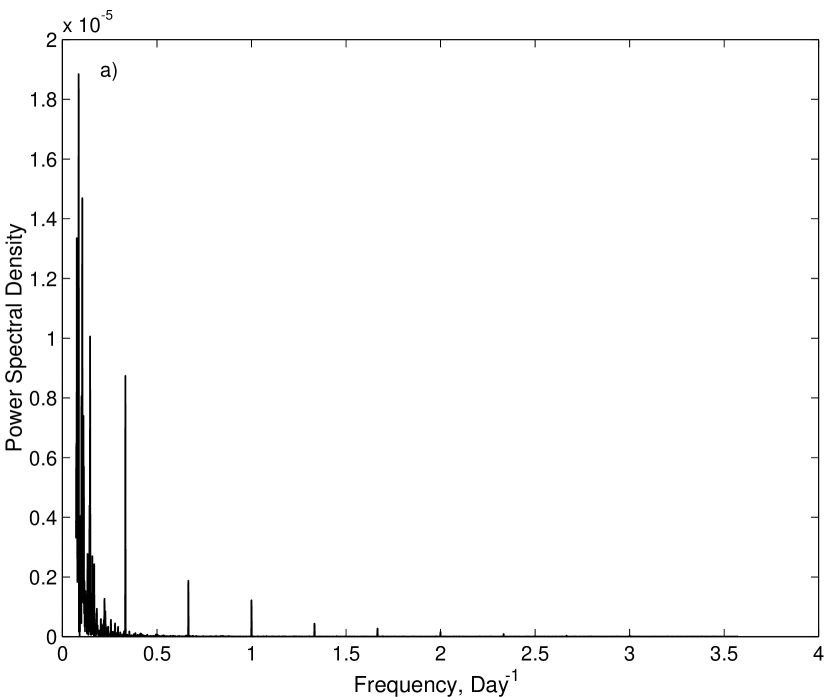
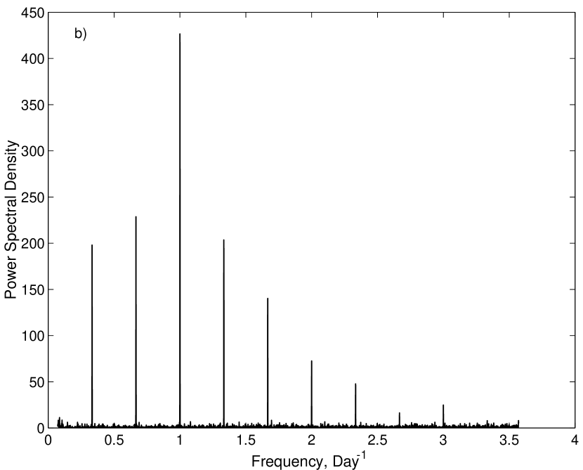
Figure 2: The process of applying the proposed detector to photometric data is illustrated by a) the periodogram of synthetic stellar variability for a solar-like star with a solar rotation period of 26.6 days, $m_{R}$=12 and an orbiting 1.2 R_J planet with an orbital period of 3 days, and b) the “whitened” periodogram. The components of the signal due to the planet appear at multiples of 1/3 day^-1. The fundamental is not the strongest component in the whitened spectrum, as it would be for the case of white observational noise.

The DIARAD measurements themselves represent a means by which the timescale-dependent response of solar-like stars to increased magnetic activity can be estimated. At solar maximum (with high magnetic activity levels), variability at long timescales increases significantly relative to solar minimum, while it remains comparatively constant at timescales of hours [see Fig. 2 of Jenkins (2002)]. Synthetic time series can be generated by transforming the DIARAD time series into the wavelet domain, scaling each timescale component by a factor which is one at the shortest timescales and that ramps up to the value indicated by the ground-based measurements for timescales $\geq 2.66$ days, followed by resampling the time series onto an appropriate grid (Jenkins, 2002). This procedure represents our best estimate of how the stellar rotation period should affect the photometric variability of solar-like stars. We do not expect this model to be accurate over a wide range of stellar types. It probably is only indicative of the expected effects over stellar types near the Sun (G1$-$G4). Warmer, late-type stars generally exhibit less spotting and consequently, lower $\sigma_{phot}$, while cooler, late-type stars exhibit more spotting and higher $\sigma_{phot}$ for a given $P_{rot}$ (see, e. g., Messina et al., 2001). Warmer, late-type stars, however, are also larger, requiring a larger planet to achieve the same S/N for a given photometric variability, while cooler, late-type stars are smaller, mitigating the increased variability for a given size planet to some degree. This analysis does not include the effects of flare events, which exhibit transient signatures on timescales of minutes (more frequently) to a few hours (more rarely), the frequency of which increases significantly for rapid rotators.

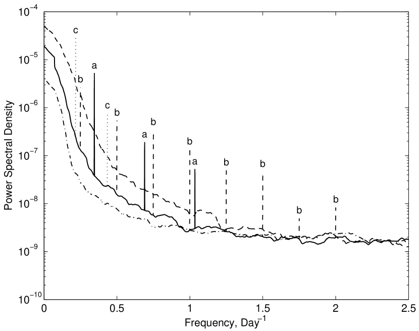
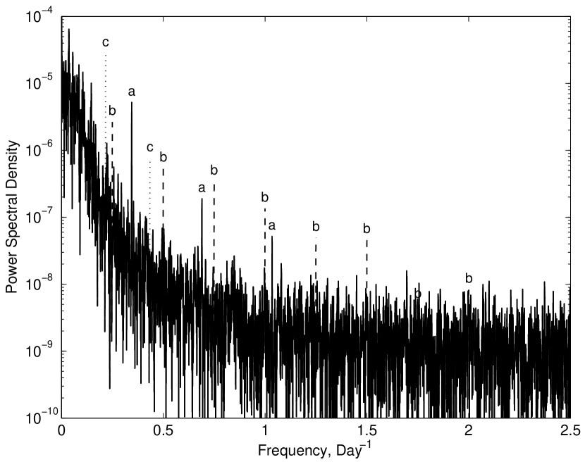
Figure 1: Power spectral density (PSD) estimates for solar-like variability and signatures of three extrasolar giant planets. Panel a) displays Hanning-windowed periodograms for a combination of the first 4 yr of the DIARAD data set and three reflected light CEGP signatures. The three planetary signatures are for 1.2 R_J planets with atmospheres composed of 1.0 $\mu$m particles in a 4 day orbit, a planet with 0.1 $\mu$m particles in a 2.9 day orbit, and a 4.6 day, albedo $p=2/3$, Lambert sphere. The planetary signatures consist of impulse trains with their harmonic components denoted by ‘a’s, ‘b’s and ‘c’s, respectively. The noise fluctuations in PSD estimates are quite evident in panel a). Three solar-like PSDs are displayed in panel b), along with a combination of these same planetary signatures and a 26.6 day period, solar-like star. The stellar PSDs have been smoothed by a 21-point moving median filter (0.015 Day^-1 wide) followed by a 195-point moving average filter (0.14 Day^-1 wide) to illustrate the average background noise. This is the procedure used by the proposed detector to estimate the background stellar PSDs prior to whitening the observed periodograms. The solid curve corresponds to the DIARAD data in panel a ($P_{rot}=26.6$ days), while the dashed and dash-dotted curves are for solar-like stars with rotation periods of 20 and 35 days, respectively, demonstrating the dependence of stellar variability on stellar rotation period. Three harmonic components of the planet with 0.1 $\mu$m particles (solid lines topped with ‘a’s) are visible above the noise in panel a), while seven components of the planet with 1.0 $\mu$m particles are visible (dashed lines topped with ‘b’s). Only two components (dotted lines topped with ‘c’s) of the $p=2/3$ Lambert sphere are visible. Thus, it should be possible to constrain the particle size distribution and composition of a CEGP atmosphere by the number of detected Fourier components. On this scale, the planetary signatures appear as vertical line segments, though they are actually distributed over a few frequency bins.

Figure 1a shows a portion of the power spectral density, PSD, for the Sun from a frequency of 0 to 2.5 day^-1. Figure 1b shows a smoothed version of the same solar PSD along with PSDs for solar-like stars with rotation periods of 20 and 35 days. The stellar PSDs in Figure 1b have been smoothed by a 21-point moving median filter (0.015 Day^-1 wide) followed by a 195-point moving average filter (0.14 Day^-1 wide) to emphasize the average background noise. The effect of decreasing $P_{rot}$ is to increase the low frequency noise and the frequency at which the PSD rolls off. The PSD for the Sun falls rapidly from 0 day^-1 to 0.25 day^-1, then gradually flattens out so that it is nearly level by 1 day^-1. Most power occurs at frequencies less than 0.1 days^-1, corresponding to the rotation of sunspots and solar-cycle variations (Frölich, 1987). On time scales of a few hours to a day, power is thought to be dominated by convection-induced processes such as granulation and supergranulation (Rabello-Soares et al., 1997; Andersen et al., 1998). At $\sim$288 day^-1, beyond the axis limits of the figure, the so-called p-modes corresponding to acoustic resonances can be observed with typical amplitudes of 10 ppm .

3 Atmospheric Models and Synthetic Reflected Light Signatures

Motivated by the upcoming microsatellite missions for studying asteroseismology, Seager et al. (2000) investigated the optical photometric reflected light curves expected for CEGPs. Their model code solves for the emergent planetary flux and temperature-pressure structure in a self-consistent fashion. The solution is found while simultaneously satisfying hydrostatic equilibrium, radiative and convective equilibrium, and chemical equilibrium in a plane-parallel atmosphere, with the impinging stellar radiation setting the upper boundary conditions. A three-dimensional Monte Carlo code computes the photometric light curves using the solution for the atmospheric profiles. For the Gibbs free energy calculations, they include 27 elements, 90 gaseous species and four solid species. These include the most important species for brown dwarfs and cool stars. The condensates, solid Fe, MgSiO₃, and Al₂O₃ are likely to be present in the outer atmospheres of the CEGPs. Four mean sizes of condensate are considered, spanning a large fraction of the range of sizes observed in planetary atmospheres in the solar system: 0.01-10 $\mu$m. Seager et al. (2000) emphasize that their study is a preliminary one, as significant improvements can be made in cloud modeling, atmospheric circulation and heat transport, photochemistry, and the inclusion of other condensates. Indeed, work to incorporate more realistic physics into these models is ongoing (Green et al., 2002)  but has not resulted in significant revisions in the general shape or amplitudes of the reflected light signatures (Sara Seager 2002, personal communication). Therefore, the published photometric light curves represent a sufficient starting point for investigating the detectability of the reflected light signatures of CEGPs and are significantly better than what can be obtained by using a Jupiter-like albedo and a simple analytic model such as a Lambert sphere.

Seager et al. (2000) find that the amplitude of the reflected light curves from CEGPs is significantly lower than that due to a Lambert sphere, which yields a signal as high as 83 ppm for a 1.2 R_J planet in a 0.051 AU orbit about a G2 star. Instead, they predict a peak flux of 22 ppm for an atmosphere consisting of a distribution of particles with a mean radius of 0.1 $\mu$m in a uniform cloud consisting of a mixture of Fe, MgSiO₃, and Al₂O₃, and at a wavelength of 0.55 $\mu$m. The scattering from these particles is at the upper limit of the Rayleigh regime, so the resulting light curve is relatively smooth. For an atmosphere composed of $\bar{r}$=1.0 $\mu$m particles, the scattering is well into the Mie regime, resulting in a strong central peak of 52 ppm centered at opposition, mainly due to backscattering from the MgSIO₃ particles at low phase angles and forward diffraction of all particles at higher phase angles, creating the steep wings at intermediate phase angles. (Seager et al., 2000) also remark that an atmosphere with stratified cloud layers would likely result in significantly higher flux reflected from the planet, as the top-level cloud would consist of MgSiO₃ because of its cooler condensation curve. For example, for $\bar{r}$=0.01 $\mu$m particles consisting of a uniform mixture of condensates, the amplitude of the reflected light signature is very low,  0.2 ppm, while for pure MgSIO₃ it is  100 times stronger. The case of $\bar{r}$=10.0 $\mu$m results in higher amplitudes for the reflected light signatures, both for the mix of the four condensates, and for pure MgSiO₃. Seager et al. (2000) consider particle sizes found in planetary atmospheres in the solar system. A $\bar{r}=$0.01 $\mu$m particle size corresponds to the haze layer above the main cloud layer in the atmosphere of Venus, which in contrast to the haze, consists of particles of size  1 $\mu$m (Knollenberg et al., 1980), while the cloud particles in Jupiter’s upper atmosphere span 0.5-50 $\mu$m (West et al., 1986). We therefore take the light curves for the uniform mixture with $\bar{r}$=0.1 $\mu$m and $\bar{r}$=1.0 $\mu$m as conservative cases for the purpose of examining photometric detectability.

The light curves given by Seager et al. (2000) can be scaled to planet-star separations different from that of 51 Peg by noting that the reflected light component amplitude is inversely proportional to the square of the star-planet separation. The authors caution that the planetary atmosphere and its cloud structure are sensitive to the insolation experienced by the planet so that this scaling law may not produce accurate results much beyond 0.05 AU or inside of 0.04 AU. They suggest, however, that the scaling law produces rough estimates at planet-star separations as high as 0.12 AU. To be complete, we also consider the detectability of CEGPs whose reflected light components are better modeled as Lambert spheres, with geometric albedos $p=0.15$ (roughly corresponding to that of Mars) and $p=2/3$ (the maximum). These light curves would likely arise from a cloudless atmosphere with a uniformly-distributed absorbing gas controlling the albedo.

4 The Kepler Mission

Kepler, a recently selected NASA Discovery Mission, is designed to detect Earth-sized planets orbiting solar-like stars in the circumstellar habitable zone. More than $100,000$ target stars will be observed in the constellation Cygnus continuously for at least 4 yr at a sampling rate of 4 hr^-1 (Borucki et al., 1997). Kepler’s aperture is 0.95 m allowing $2.21\times 10^{8}~{}e^{-}$ to be collected every 15 minutes for a G2, $m_{R}=12$ dwarf star with a shot noise of 67 ppm. The instrument noise itself should be $\sim$ 31 ppm over this same duration. This value is based on extensive laboratory tests, numerical studies and modeling of the Kepler spacecraft and photometer (Koch et al., 2000; Jenkins et al., 2000b; Remund et al., 2001). The values in Table 3 of Koch et al. (2000) support this level of instrumental noise from a high-fidelity hardware simulation of Kepler’s environment, while the numerical studies of Remund et al. (2001) are based on a detailed instrumental model. This model includes noise terms such as dark current, read noise, amplifier and electronics noise sources, quantization noise, spacecraft jitter noise, noise from the shutterless readout, cosmic ray hits, radiation damage accumulated over the lifetime of the mission, and the effects of charge transfer efficiency.

To simulate the combined effects of the shot noise and instrumental noise for $Kepler$, white Gaussian noise (WGN) sequences were added to the DIARAD time series with a standard deviation equal to the square root of the combined shot and instrumental variance for a star at a given magnitude less the square of the DIARAD instrumental uncertainty [$0.1~{}W~{}m^{-2}$ in each 3 minute DIARAD measurement (Steven Dewitte 1999, personal communication)]. For example, the combined instrumental and shot noise for a $m_{R}$=12 star at the 15 minute level is $\sim$74 ppm, but the DIARAD instrumental noise is $\sim$33 ppm, so the appropriate standard deviation for the WGN sequence is 66 ppm.

The Kepler Mission should not suffer from large time gaps. Roll maneuvers are planned about every 90 days to reorient the sunshade and the solar panels, resulting in a loss of $\sim$1% of the total data. While the simulations discussed in §6 do not include the effect of the missing data, it should be small and can be accommodated directly into a tapered spectrum estimate as per Walden et al. (1998).

5 A Galactic Model for the Distribution of Kepler Target Stars

Along with characterizations of stellar variability as a function of stellar rotation period, $P_{rot}$, and a characterization of the observation noise for Kepler, we require a model for the distribution of Kepler’s main-sequence target stars as functions of apparent magnitude, spectral type, and age. Combined with a characterization of the detectability of CEGPs with respect to apparent brightness and $P_{rot}$, the stellar distribution allows for the performance of the proposed detector to be optimized and evaluated (§6 and §7). In addition, a model of the distribution of dim background stars in the FOV permits an analysis of the problem of confusion (§9).

Following Batalha et al. (2002), we make use of galactic models made publicly available by the Observatoire de Besançon (see, e. g., Robin & Crézé, 1986; Haywood, Robin, & Crézé, 1997a, b) to obtain expected main sequence starcounts as a function of apparent magnitude, spectral type and age. The USNO-A2.0 database yields 223,000 stars to $m_{R}$=14.0 in the 106 square degrees of Kepler’s FOV (David Koch 2001, personal communication). This establishes an appropriate mean extinction of $\sim$1.0 mag $\mathrm{kpc}^{-1}$ for the Besançon model. We note, however, that the bandpass for Kepler extends from $\sim$0.45 to $\sim$0.85 $\mu$m, which is far wider than the bandpasses available for the Besançon models. For the purpose of counting stars, using the R band should reflect the number of stars of greatest interest, but may tend to undercount the number of late main sequence stars. The age-rotation relation formulated by Kawaler (1989) then permits us to rebin the starcounts obtained from the Besançon model with respect to rotation period rather than stellar age, for which we can evaluate the expected detection rates. This relation is given by

$$\log(P_{rot})=0.5\log(t_{0})+0.390(B-V)+0.824,$$ (2)

where $P_{rot}$ is stellar rotation period in days, $t_{0}$ is stellar age in Gyr, and B and V are the blue and visible photometric brightnesses in the Johnson UBVRI system, respectively. For this exercise, the apparent magnitudes were binned into 1 magnitude intervals with central values from $m_{R}$=9.5 to 14.5, the spectral type bins were centered on spectral types B5, A5, F5, G5, K5, and M5, and the rotation periods were binned into 5 day intervals from 5 to 40 days. Stars rotating with periods outside this range were set to the respective edge bin values.

Table 1 gives the number of stars in each spectral type and apparent magnitude bin. The Observatoire de Besançon galactic model estimates that there are $\sim$80,000 main sequence stars to $m_{R}$=14.0 and $\sim$220,000 main sequence stars to $m_{R}$=15.0 in Kepler’s FOV. Other models exist that predict higher fractions of main-sequence stars (David Koch 2002, personal communication), so that this is a reasonably conservative starting point. There are 14 extrasolar planets currently known with orbital periods less than 7 days: four with periods of nearly 3.0 days, four with periods of $\sim$3.5 days, and the remaining six are approximately uniformly distributed between $P$=4 and 6.4 days. About 0.75% of solar-like stars possess planets with periods between 3 and 5 days (Butler et al., 1999), which we scale to 0.875% since two of the CEGPs for our model distribution have periods greater than 5 days. Taking this value for the fraction of target stars that possess CEGPs, we obtain the results listed in Table 2, for a total of 693 planets to $m_{R}$=14.0 and 1,807 planets to $m_{R}$=15.0. Of these, $\sim$10% should exhibit transits, as given in Table 3. The photometric signals from these transiting planets will be huge compared to the measurement noise, so that virtually all of these planets whose parent stars are observed by Kepler will be detected. Thus, there should be $\sim$44 CEGPs to $m_{R}$=14.0 and 181 CEGPs to $m_{R}$=15.0 discovered within the first several weeks of observation. The question addressed throughout the remainder of this paper is, how many additional planets should Kepler be able to detect by reflected light?

6 Detection Approach

The detection of reflected light signatures of non-idealized model atmospheres such as those predicted by Seager et al. (2000) is more complicated than for the signature of a Lambert sphere. The power spectrum of any periodic waveform consists of a sequence of evenly spaced impulses separated by the inverse of the fundamental period. For a Lambert sphere, over 96% of the power in the reflected light component is contained in the fundamental (aside from the average flux or DC component, which is undetectable against the stellar background for non-transiting CEGPs). Thus, detecting the reflected light signature of a Lambert sphere can be achieved by forming the periodogram of the data, removing any broadband background noise, and looking for anomalously high peaks. In contrast, the power of the Fourier expansions of Seager et al.’s model CEGP light curves at high orbital inclinations is distributed over many harmonics in addition to the fundamental due to their non-sinusoidal shapes (see Fig. 1). How does one best search for such a signal?

As in the case of a pure sinusoid, a Fourier-based approach seems most appropriate, since the Fourier transform of a periodic signal is strongly related to its Fourier series, which parsimoniously and uniquely determines the waveform. Unlike the case for ground-based data sets that are irregularly sampled and contain large gaps, photometric time series obtained from space-based photometers like Kepler in heliocentric orbits will be evenly sampled and nearly complete. This removes much of the ambiguity encountered in power spectral analysis of astronomical data sets collected with highly irregular or sparse sampling. Thus, power spectral analyses using Fast Fourier Transforms (FFTs) simplify the design of a detector. For the sake of this discussion, let $x(n)$ represent the light curve, where $n\in\{0,\ldots,N-1\}$ is an $N$-point time series with a corresponding discrete Fourier transform (DFT) $X(k)$, $\omega=2\pi\,k/N$ is angular frequency, and $k\in\{0,\ldots,N-1\}$). The phase of the light curve is a nuisance parameter from the viewpoint of detecting the planetary signature and can be removed by taking the squared magnitude of the DFT, $P_{X}(k)=|X(k)|^{2}$, which is called the periodogram of the time series $x(n)$. In the absence of noise, if the length of the observations were a multiple of the orbital period, $T_{p}$, then the periodogram would be zero everywhere except in frequency bins with central frequencies corresponding to the inverse of the orbital period, $f_{0}=T_{p}^{-1}$, and its multiples. If the length of the observations is not an integral multiple of the orbital period, the power in each harmonic is distributed among a few bins surrounding the true harmonic frequencies, since the FFT treats each data string as a periodic sequence, and the length of the data is not consonant with the true orbital period. The presence of wide-band measurement noise assures that each point in the periodogram will have non-zero power. Assuming that the expected relative power levels at the fundamental and the harmonics are unknown, one can construct a detection statistic by adding the periodogram values together that occur at the frequencies expected for the trial period $T_{p}$, and then threshold the summed power for each trial period so that the summed measurement noise is not likely to exceed the chosen threshold. The statistic must be modified to ensure that it is consistent since longer periods contain more harmonics than shorter ones, and consequently, the statistical distribution of the test statistics depends on the number of assumed harmonics. This is equivalent to fitting a weighted sum of harmonically related sinusoids directly to the data. Kay (1998) describes just such a generalized likelihood ratio test (GLRT) for detecting arbitrary periodic signals in WGN assuming a generalized Rayleigh fading model.

The approach we consider is similar; however, we assume the signals consist of no more than seven Fourier components, and we relax the requirement that the measurement noise be WGN. This is motivated by the observation that the model light curves developed by Seager et al. (2000) are not completely arbitrary and by the fact that the power spectrum of solar-like variability is very red: most of the power is concentrated at low frequencies. At low inclinations, the reflected light curves are relatively smooth and quasi-sinusoidal, exhibiting few harmonics in the frequency domain. At high inclinations, especially for the $\bar{r}$=1.0 $\mu$m model, the presence of a narrow peak at opposition requires the presence of about seven harmonics in addition to the fundamental (above the background solar-like noise). Another GLRT approach would be to construct matched filters based directly on the atmospheric models themselves, varying the trial orbital period, inclination, mean particle size, etc. A whitening filter would be designed and each synthetic light curve would be “whitened” and then correlated with the “whitened” data. We choose not to do so for the following reason: These models reflect the best conjectures regarding the composition and structure of CEGP atmospheres at this time, with little or no direct measurements of their properties. A matched filter approach based on these models could potentially suffer from a loss in sensitivity should the actual planetary atmospheres differ significantly from the current assumptions. On the other hand, the general shape and amplitude predicted by the models are likely to be useful in gauging the efficiency of the proposed detector.

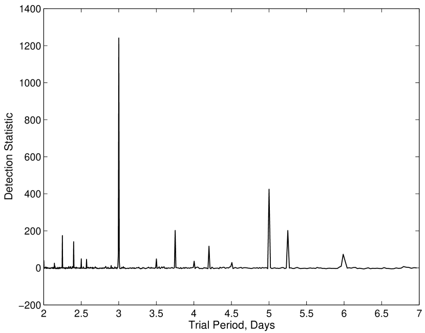
Figure 3: The co-added spectrum corresponding to the time series in Fig. 2 is shown. The periodogram has been co-added to itself so that the components of a periodic signal appear in the same bin, and thus, dramatically increase the chance of detection. Note the strong peak at 3 days, corresponding to the period of the signal in the time series. This may not always be the case as it depends on the strength of the fundamental compared to the background stellar and instrumental noise. In any case, the presence of many strong peaks at rational harmonics of the actual fundamental provide additional confidence that a periodic signal has been detected, and their spacing dictates the fundamental period.

Our detector consists of taking the periodogram as an estimate of the power spectral density (PSD) of the observations, estimating the broadband background power spectrum of the measurement noise, “whitening” the PSD, and then forming detection statistics from the whitened PSD. We first form a Hanning-windowed periodogram of the $N$-point observations. For convenience, we assume the number of samples is a power of 2. For Kepler’s sampling rate, $f_{s}$=4 hr^-1, $N=2^{17}$ points corresponds to 3.74 yr or about 4 yr. The broadband background, consisting of stellar variability and instrumental noise, is estimated by first applying a 21-point moving median filter (which replaces each point by the median of the 21 nearest points), followed by applying a 195-point moving average filter (or boxcar filter). The moving median filter tends to reject outliers from its estimate of the average power level, preserving signatures of coherent signals in the whitened PSD. The length of 195 points for the moving average corresponds to the number of frequency bins between harmonics of a 7 day period planet for the assumed sampling rate and length of the observations. Both of these numbers are somewhat arbitrary: wider filters reject more noise but don’t track the power spectrum as well as shorter filters do in regions where the PSD is changing rapidly. This background noise estimate is divided into the periodogram point-wise, yielding a “whitened” spectrum as in Figure 2. The advantage of whitening the periodogram is that the statistical distribution of each frequency bin is uniform for all frequencies except near the Nyquist frequency and near DC (a frequency of 0), simplifying the task of establishing appropriate detection thresholds. The whitened periodogram is adjusted to have an approximate mean of 1.0 by dividing it by a factor of 0.6931, the median of a $\chi_{2}^{2}(2x)$ process. (This adjustment is necessitated by the moving median filter.) Finally, the value 1 is subtracted to yield a zero-mean spectrum. [The distribution of the periodogram of zero-mean, unit-variance WGN is $\chi_{2}^{2}(2x)$ (see, e. g., Papoulis, 1984).] Finally, the detection statistic for each trial period $N/\left(Kf_{s}\right)$ is formed by adding the bins with center frequencies $iKf_{s}/N$, $i=1,\ldots,M$ together, where $M\leq 7$, as in Figure 3. The trial periods are constrained to be inverses of the frequency bins between 1/2 and 1/7 days^-1.

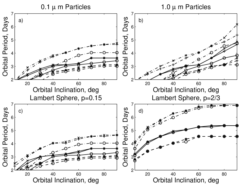
Figure 4: The maximum detectable planetary period at a detection rate of 90% vs. orbital inclination for various stellar brightnesses and rotation periods and 4 yr of data are plotted for: a) Seager et al.’s $\bar{r}=0.1$ $\mu$m particle model, b) Seager et al.’s $\bar{r}=1.0$ $\mu$m particle model, c) a Lambert sphere with geometric albedo $p=0.15$, and d) a Lambert sphere with $p=2/3$. The number of assumed Fourier components, $M$, is set to one here. Stellar rotation periods of 20 days, 25 days and 35 days are denoted by dashed lines, solid lines and dash-dotted lines, respectively. Stellar magnitudes $m_{R}$=9.5, 11.5 and 13.5 are denoted by ‘x’s, crosses, and open circles, respectively. The first three models yield comparable numbers of expected CEGP detections. Seager et al.’s $\bar{r}=1.0$ $\mu$m particle model is easier to detect at longer periods at high orbital inclinations relative to the $\bar{r}=0.1$ $\mu$m particle model or the $p=0.15$ Lambert sphere model. This is due to the greater number of Fourier components, which can compensate for red noise from stellar variability that can mask lower frequency harmonics.

This procedure was applied to each of 450 model reflected light curves spanning inclinations from 10^∘ to 90^∘, orbital periods from 2 to 7 days, plus stellar variability for stars with $P_{rot}$ between 5 and 40 days and instrumental and shot noise corresponding to apparent stellar brightnesses between R=9.0 and R=15.0. The combinations of these parameters generated a total of 21,600 synthetic PSDs for which the corresponding detection statistics were calculated. The number of assumed Fourier components was varied from $M=1$ to $M=7$. Some results of these numerical trials are summarized in Figure 4, which plots the maximum detectable orbital period, $P_{\mathrm{max}}$, for $M=1$ at a detection rate of 90% against $I$, for $P_{rot}$=20, 25 and 35 days, for Sun-like (G2V) stars with apparent stellar magnitudes $m_{R}$=9.5, 11.5 and 13.5. Detection thresholds and detection rates are discussed in §7.

For $\bar{r}=0.1$ $\mu$m clouds (Fig. 4a), planets are detectable out to $P=4.75$ days for $P_{rot}$=35 days, out to $P=3.7$ days for $P_{rot}=25$ days, and out to $P=3.1$ days for $P_{rot}=20$ days. The curves are rounded as they fall at lower inclinations, and planets with $I$ as low as 50^∘ are detectable for all the curves, while planets with $I>20^{\circ}$ are detectable only for stars with $P_{rot}=35$ days. For clouds consisting of $\bar{r}=1.0$ $\mu$m particles (Fig. 4b), the curves of $P_{\mathrm{max}}$ are more linear, extending to orbital periods as long as 6 days for $P_{rot}=35$ days, as long as 4.8 days for $P_{rot}=25$ days, and to $>3$ days at high inclinations for stars brighter than $m_{R}$=14. The detectability of both of these models at high orbital inclinations would be improved by searching for more than one Fourier component, (i. e., choosing a higher value for $M$). This is a consequence of the larger number of harmonics in the reflected light signature. Although the power is distributed among more components, as the orbital period increases, the signal is less sensitive to the low frequency noise power due to stellar variability, which easily masks the low frequency components of the signal. The behavior of the maximum detectable planetary radius for a Lambert sphere with $p=0.15$ (Fig. 4c) is very similar to Seager et al.’s $\bar{r}=0.1$ $\mu$m model. A Lambert sphere with $p=2/3$ outperforms all the other models, as expected due to its significantly more powerful signal. Planets in orbits up to nearly 7 days can be detected for Sun-like stars with rotation periods of 35 days. For Sun-like stars with rotation periods of 25 and 20 days, planets are detectable with orbital periods up to 5.4 and 4.6 days, respectively. The Lambert sphere model PSD’s contain only two Fourier components. Consequently, the detectability of such signatures is not improved significantly by choosing $M>1$.

Now that we have specified the detector, we must analyze its performance for the stellar population and expected planetary population. We should also determine the optimal number, $M_{\mathrm{opt}}$, of Fourier components to search for, if possible. The value of doing so cannot be overstated: higher values of $M$ require higher detection thresholds to achieve a given false alarm rate. If too large a value for $M$ is chosen then adding additional periodogram values for $M>M_{\mathrm{opt}}$ simply adds noise to the detection statistic. This will drive down the total number of expected detections. On the other hand, if too small a value for $M$ is chosen, then the sensitivity of the detector to CEGP signatures would suffer and here, too, the number of expected detections would not be maximized. The first step is to determine the appropriate threshold for the desired false alarm rate as a function of $M$. This is accomplished via Monte Carlo runs as presented in §7. To determine the best value of $M$, we also need a model for the population of target stars, which defines the observation noise, and a model for the distribution of CEGPs. We use the Besançon galactic model to characterize the target star population (§5). The distribution of CEGPs with orbital period can be estimated from the list of known CEGPs. Moreover, we need a method for extrapolating solar-like variability from that of the Sun to the other spectral types. Two methods are considered and discussed in §8. In the first, the stellar variability is treated strictly as a function of stellar rotation period, so that the detection statistics are adjusted for the varying stellar size. In the second, it is assumed that the mitigating effects of decreasing (increasing) the stellar area towards cooler (warmer) late-type stars are exactly balanced by an increase (decrease) in stellar variability. Hence, no adjustment is made to the detection statistics as a function of spectral type. Given this information, we can then determine which value of $M$ maximizes the number of expected CEGP detections for a particular atmospheric model.

We found that the optimal value of $M$ depends a great deal on the assumed stellar population, and the distribution of CEGPs with orbital period. If the rotation periods of Kepler’s target stars were evenly distributed, then optimal values for $M$ varied from $M=1$ to $5$, depending on the atmospheric model and method for extrapolating stellar variability across spectral type. Adopting a realistic distribution of stellar rotation period and spectral type produced a surprising result. We found that $M=1$ yielded the highest number of detections assuming all four of the atmospheric models considered were equally likely. The number of detections for each atmospheric model as a function of $M$, and the average number of detections across all four atmospheric models are given in Table 4. The results of both methods for extrapolating stellar variability across spectral type are averaged together for this exercise. The effects of setting $M$ to 1 were not strong for Seager et al.’s $\bar{r}$=1.0 $\mu$m model where $M_{\mathrm{opt}}$ exceeded 1. In this case, $M=2$ or 3 was optimal, depending on how stellar variability was extrapolated. Up to 6% fewer CEGPs would be detected using $M=1$ rather than $M=3$ (174 vs. 185 total detections). For Seager et al.’s $\bar{r}=$0.1 $\mu$m model and both Lambert sphere models, $M=1$ was optimal, although the average number of detections drops slowly with $M$.

7 Monte Carlo Analysis

In order to determine the detection thresholds and the corresponding detection rates, we performed Monte Carlo experiments on WGN sequences. Much of this discussion draws on that of Jenkins et al. (2002), which concerns the analogous problem of establishing thresholds for transit searches. Each random time series was subjected to the same whitening, and spectral co-adding as described in §6. Two statistical distributions produced by these Monte Carlo trials are of interest: that of the null statistics for a single trial period, and that of the maximum null statistic observed for a search over all the trial periods. The former defines in part the probability of detection for a given planetary signature and background noise environment, since the distribution of the detection statistic in the presence of a planet can be approximated by shifting the null distribution by the mean detection statistic. The latter dictates the threshold necessary to control the total number of false alarms for a search over a given number of stars.

Let $l_{1,0}(M)$ denote the random process associated with the null statistics for a single trial period, and assumed number of Fourier components, $M$. Likewise, let $l_{\mathrm{max},0}(M)$ denote the random process corresponding to the null statistics for a search of a single light curve over all trial periods. The corresponding cumulative distribution functions are $P_{l_{1,0}}(x,M)$ and $P_{l_{\mathrm{max},0}}(x,M)$, respectively. For $N_{*}$ stars, the thresholds, $\eta(M)$, that yield a false alarm rate of $1/N_{*}$ for each search are those values of $x$ for which

$$Q_{l_{\mathrm{max},0}}(x,M)=1-P_{l_{\mathrm{max},0}}(x,M)=1-1/N_{*}$$ (3)

and hence, deliver a total expected number of false alarms of exactly one for a search of $N_{*}$ light curves. For a given threshold, $\eta$, and mean detection statistic, $\bar{l}_{1}(M)$, corresponding to a given planetary signature the detection rate, $P_{D}(M)$, is given by

$$P_{D}(M)=P_{l_{1,0}}(\bar{l}_{1}-\eta,M),$$ (4)

where the explicit dependence of $\bar{l}_{1}$ and $\eta$ on $M$ is suppressed for clarity.

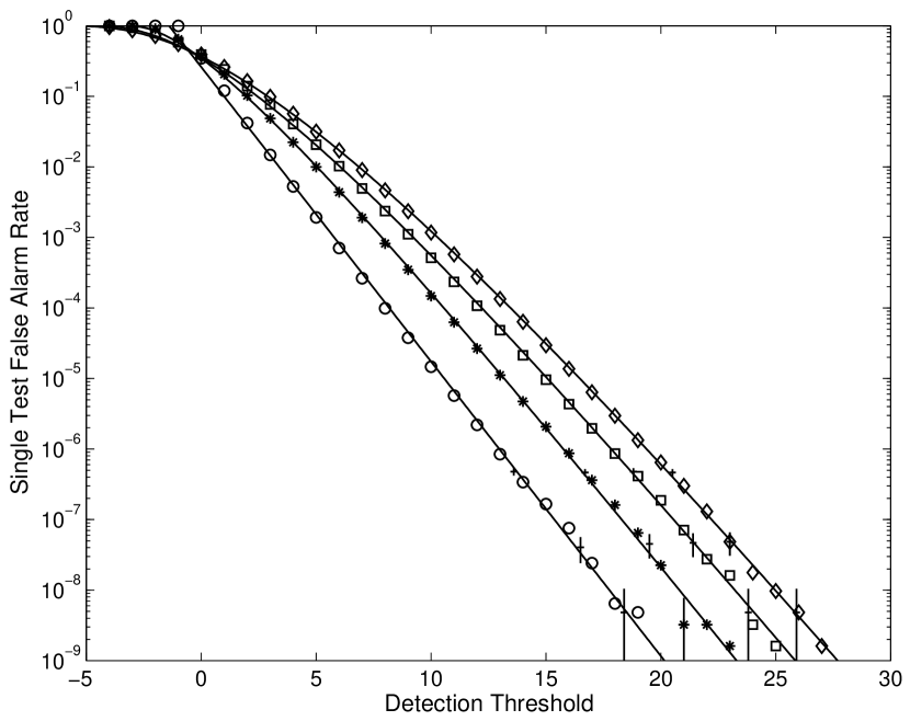
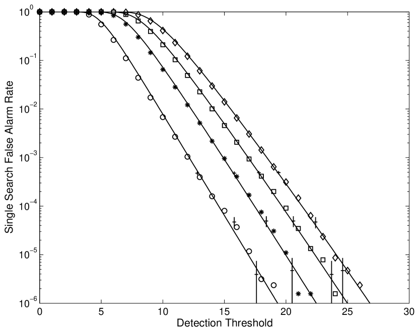
Figure 5: The single test a) and single search b) false alarm rates as functions of detection threshold for the proposed detector. The number of assumed Fourier components, $M$=1, 3, 5 and 7, are denoted by circles, asterisks, squares, and diamonds, respectively, for the sample distributions. For clarity, only every fifth point of each sample distribution is plotted. The solid curves indicate the least-squares fits to the log of the sample distributions, emphasizing the upper tail in the fit. Error bars for 95% confidence intervals are denoted by vertical line segments crossed by horizontal line segments at various locations in each sample distribution. The single test false alarm rates can be used to estimate the detection rates for a given CEGP signal (see Fig. 6), while the single search false alarm rates determine the detection threshold for a given number of target stars and desired total number of false alarms. Determining the optimal value of $M$ is important, given that higher values of $M$ require correspondingly higher detection thresholds, which drives down the number of detections if the chosen value of $M$ is too high.

Figure 5a shows the sample distributions for $Q_{l_{1,0}}(x,M)$ resulting from 619 million Monte Carlo trials for $M=1$, 3, 5, and 7. This represents the single test false alarm rate as a function of detection threshold. Figure 5b shows $Q_{l_{\mathrm{max},0}}(x,M)$ resulting from 1.3 million Monte Carlo runs, for the same values of $M$. This represents the single search false alarm rate as a function of detection threshold for each value of $M$. Error bars denoting the 95% confidence intervals appear at selected points in both panels.

It is useful to model $P_{l_{1,0}}$ and $Q_{l_{\mathrm{max},0}}$ analytically. If the whitening procedure were perfect, and assuming that the observation noise were Gaussian (though not necessarily white), $l_{1,0}$ would be distributed as a $\chi^{2}_{2\,M}$ random variable with a corresponding distribution $Q_{\chi^{2}_{2\,M}}(2\,x+2\,M)$. Figure 5a shows the sample distributions for $l_{1,0}$ resulting from 619 million Monte Carlo runs. Higher values of $M$ require higher thresholds to achieve a given false alarm rate. We fit analytic functions of the form

$$Q_{l_{1,0}}(x,M)\approx Q_{\chi^{2}_{2\,M}}(A\,x+B)$$ (5)

to the sample distributions $Q_{l_{1,0}}(x,M)$, where parameters $A$ and $B$ allow for shifts and scalings of the underlying analytical distributions. Two methods for determining the fitted parameters are considered. In the first, we fit the analytic expressions directly to the sample distributions, including the uncertainties in each histogram bin. The resulting fit is useful for estimating the detection rate as a function of signal strength above the threshold, but may not fit the tail of the distribution well. In the second method, the log of the analytic function is fitted to the log of the sample distributions in order to emphasize the tail. The fitted parameters are given in Table 5. Regardless of whether the sample distribution or the log sample distribution is fitted, the values for $A$ are within a few percent of 2 and the values of $B$ are no more than 14% different from $2\,M$, indicating good agreement with the theoretical expectations.

To determine the appropriate detection thresholds, we need to examine the sample distributions $Q_{l_{\mathrm{max},0}}$. These are likely to be well-modeled as the result of taking the maximum of some number, $N_{\mathrm{EIT}}$, of independent draws from scaled and shifted $\chi^{2}_{2\,M}$ distributions. Here, $N_{\mathrm{EIT}}$ is the effective number of independent tests conducted in searching for reflected light signatures of unknown period in a single light curve. We take the values for $A$ and $B$ obtained from the fits to the log of $Q_{l_{1,0}}(x,M)$ and fit the log of the analytic functions of the form

$$Q_{l_{\mathrm{max},0}(x,M)}\approx 1-P_{\chi^{2}_{2\,M}}^{N_{\mathrm{EIT}}}\left(A,x+B\right)$$ (6)

to the log of the sample distributions $Q_{l_{\mathrm{max},0}}(x,M)$. The values for $N_{\mathrm{EIT}}$ are given in Table 5 and fall between 430 and 476. For the length of data considered, there are $\sim$490 frequency bins corresponding to periods between 2 and 7 days. Thus the whitening and spectral co-adding operations apparently introduce some correlation among the resulting detection statistics, somewhat reducing the total number of independent tests conducted per search.

In determining the expected number of CEGPs whose reflected light signatures Kepler will likely detect, we average the detection rates from §6 over all inclinations and over the distribution of planetary periods of known CEGPs (see §5). The former can be accomplished by noting that inclination for randomly oriented orbits is distributed according to the sine function. Table 6 contains the average detection rates for 1.2 R${}_{\mathrm{J}\,}$planets orbiting Sun-like stars as functions of stellar rotation period and apparent magnitude for all four atmospheric models for a detector with $M=1$. These results correspond to a false alarm rate of 1 in $10^{5}$ light curve searches. The detection rate falls more rapidly with decreasing stellar rotation period than it does with increasing apparent stellar magnitude for the range of magnitudes and rotation periods considered here. The atmospheric models predicted by Seager et al. (2000) are sensitive to the planet-star separation and are not likely to be accurate for planets well within 0.04 AU or planets much beyond 0.05 AU. Most of the planets making up our assumed planetary orbit distribution function fall within or close to these limits. Thus, we do not believe that departures from the simple scaling suggested by Seager et al. (2000) are important in estimating the number of CEGPs that Kepler will detect. The detection rate is zero for stars with rotation periods shorter than 20 days for all save the $p=2/3$ Lambert sphere model which can detect planets orbiting stars with $P_{rot}$ as short as 15 days.

8 Expected Number of Detections

In this section we use the results of §5, §6 and §7 along with statistics of the known CEGPs to estimate the expected number of detections of CEGPs by reflected light for Kepler. As discussed in §6, the results depend on $M$, the assumed number of harmonics in the CEGP light curve. Here we discuss in detail only the results obtained by setting $M=1$, which maximized the number of detections assuming all four atmospheric models were equally likely. Throughout this discussion we assume a uniform radius of 1.2 R_J for all CEGPs. This is somewhat conservative: the only CEGP with a known radius is the celebrated case of HD209458b with a radius of 1.4 R_J (Cody & Sasselov, 2002).

Two methods to extrapolate stellar variability as a function of spectral type are considered. In the first, we assume that the relationship between rotation period and stellar variability holds for all spectral types, so that we modify the detection rates by accounting for the dependence on the signal amplitude with the area of the star, $R_{*}^{-2}$. That is, the PSD of stellar variability is assumed to be a function of stellar rotation period alone, while the amplitude of the planetary signature also depends on the size of the star. We denote this method as spectral type compensation method A. The second method, B, starts with the general observation that warmer late-type stars tend to be more photometrically quiescent than cooler late-type stars at time scales relevant to detecting CEGPs and further assumes that this relationship compensates exactly for the dependence of signal strength on stellar radius. That is, for this model, no adjustment for stellar radius is made to the amplitude of the planetary signature. The validity of these approaches will be tested by Kepler and the other upcoming photometry space missions. An important point is that the proposed detector can be tuned to the actual observation noise via Monte Carlo techniques since CEGPs are relatively rare. The two approaches considered here are not expected to be 100% valid, but should produce reliable estimates for the number of CEGPs Kepler can expect to detect.

The expected number of CEGPs detected under spectral type compensation method A are given in Table 7, which lists the number of detected planets for each of the four planetary atmospheric models. Seager et al.’s $\bar{r}$=1.0 $\mu$m and $\bar{r}$=0.1 $\mu$m models, and the Lambert sphere model with $p=0.15$ all detect about the same number of planets: $\sim$120 to $m_{R}=14.0$ and $\sim$220 to $m_{R}$=15.0. For G-type stars, $\sim$65 CEGPs to $m_{R}$=14.0 and $\sim$114 CEGPs to $m_{R}$=15.0 should be detected for each of these models. Among the four atmospheric models and spectral type compensation method A, the Lambert sphere model with $p=2/3$ stands out. In this case, 230 and 712 CEGPs would be detected to $m_{R}$=14.0, and $m_{R}$=15.0, respectively. A little over half of these detections would occur around G-type stars. In contrast to the other atmospheric models, significant numbers of CEGPs would be detected around F-type stars, in addition to G-, K- and M-type stars.

Table 8 contains the estimates for the number of CEGPs detected under spectral type compensation method B. Here, for Seager et al.’s models and for the $p=0.15$ Lambert sphere, the number of expected detections drop by about $\sim$40% to $m_{R}$=14.0 and by $\sim$50% to $m_{R}$=15.0. About 80 planets are detected to $m_{R}$=14.0 ($\sim$55 orbiting G-type stars), and $\sim$115 planets are detected to $m_{R}$=15.0 ($\sim$80 orbiting G-type stars). In contrast, the $p=2/3$ Lambert sphere model detects $\sim$8% more planets than it does for method A. The reason for the differences between method A and method B is that the detections are shifted to earlier type stars. The $p=2/3$ Lambert sphere model gains detections because there are more F-type target stars than G-type target stars according to the galactic model, which offsets the lower detectability of the CEGP signal for the faster rotating F stars. The detectabilities of the CEGP signals for the other atmospheric models are more sharply reduced for F stars, so that while the detections shift towards F stars, an insufficient number are gained to offset the reduced number of detections for later star types.

As expected, more detections are obtained if stars as dim as $m_{R}$=15.0 are observed. There are 132,000 more stars between $m_{R}$=14.0 and $m_{R}$=15.0 than there are to $m_{R}$=14.0 ($\sim$80,000), for a total of $\sim$200,000 main-sequence stars in the FOV. Kepler’s downlink and onboard storage system are capable of handling $\sim$200,000 target stars for the first year of operation, and $\sim$140,000 thereafter. The most promising targets are those stars with long rotation periods. This can be ascertained after several months of observation once a good PSD estimate can be obtained and the detection rates can be estimated. It is likely that the $\sim$200,000 main sequence stars to $m_{R}$=15.0 in Kepler’s FOV can be pared down to $\sim$140,000 during the first year of observation. Thus, Kepler can be expected to detect the reflected light signatures of between 100 and 760 CEGPs (see Tables 7 and 8). Note that the detections should be evenly distributed in time: the energy of a reflected light signature is directly proportional to the length of its time series. Thus, approximately 25% of the discoveries, or between 25 and 190 CEGPs should be detected by reflected light within the first year of the Kepler Mission.

The highest detection rates occur for edge-on planetary orbits: those most likely to produce transits. Between 14% and 40% of the CEGPs detected by reflected light will exhibit transits, depending on the assumed atmospheric model and stellar variability model. These planets present an opportunity to extract the shape of the occultation of the planet by its star. In this case, the average brightness or DC level of the reflected light signature can also be determined, which is not the case for non-transiting CEGPs. Moreover, since the transits will almost certainly be detected in the first several weeks of the mission, the requisite thresholds for detecting the reflected light signatures can be significantly reduced, since the period is constrained by the observations of the transits. Given that $\sim$181 CEGPs in the FOV will exhibit transits, we should be able to constrain if not measure the albedos quite well.

While solar variability may certainly not be safely extrapolated to significantly different stellar classes, detections of CEGPs might also be possible around G3 through early K giants because of their expected low rotation rates, if the rotation period criteria in this study is found to be applicable to giant stars. M giants might be too large to allow very close planets (see, e. g., Gray, 1992), however K giants, because of their increased mass, would allow planets 50% more distant with the same orbital periods discussed above.

9 Potential Sources of Confusion and Methods of Discrimination

Detection algorithms detect all signals of sufficient amplitude with features that are well matched to the shape of the signal of interest. Thus, not all signals yielding detection statistics above the detection threshold need be signatures of CEGPs. Indeed, several potential sources of confusion exist that might inject signals similar to reflected light signatures of CEGPs. These include intrinsic photometric variability of target stars themselves, and dim background variable stars within the photometric apertures of target stars. Such variations include those produced by star spots, eclipsing or grazing eclipsing binaries, or intrinsic stellar pulsations. Section §9.1 describes each of these classes of variability along with an assessment of the likelihood they pose as sources of confusion. Section §9.2 presents a robust method for rejecting confusion from blended, variable background stars in a target star’s photometric aperture.

9.1 Potential Sources of Confusion

Sources of stellar variability that might be mistaken for reflected light signatures of CEGPs include stellar pulsations, star spots, and photometric variability induced by binarity. These phenomena can occur in the target star or in a blended background star, but the amplitudes of concern are different since the magnitude of the variations of a blended background star will be diluted by the flux of the target star. In addition, non-reflected light signatures of CEGPs might be present, confounding the isolation and detection of the reflected light signature. In this section we discuss these sources of photometric variability and assess the likelihood that each poses as a source of confusion.

CEGPs can induce periodic photometric variations other than that due to reflected light. Doppler modulation of the host stellar spectrum via reflex motion of the host star about the system barycenter modulates the total flux observed in the photometer’s bandpass. Loeb & Gaudi (2003) estimate the amplitude of this effect and conclude that Doppler-induced photometric variations for Jupiter-mass planets orbiting solar-type stars in periods less than 7 days are about 20 times fainter than the reflected light signature of Jupiter-sized, $p=2/3$ Lambert spheres. The Doppler-induced photometric signal is 90^∘ out of phase with that of the reflected light component from a CEGP. Hence, rather than making it more difficult to detect a CEGP, the combination of the two signatures makes it easier to detect one since the power from orthogonal signals add constructively in the frequency domain. Radial velocity measurements should help distinguish between the two signatures in the case of non-transiting CEGPs.

Stellar pulsations can cause strictly periodic photometric variations. Acoustic waves traveling in the Sun resonate at specific frequencies with characteristic periods on the order of 5 minutes and typical amplitudes of $\sim$10 ppm. The coherence lifetime for these so-called p-mode oscillations is approximately a month, beyond which the sinusoidal components drift out of phase (Deubner, 1984). Buoyancy waves (also called gravity waves) should have much longer periods of 0.28-2.8 hours along with correspondingly longer coherence timescales. To date, no one has observed the signatures of g-modes in the Sun. The VIRGO experiment aboard SOHO has placed upper limits of 0.5 ppm on the amplitudes of solar g-modes (Appourchaux et al., 2000), which is in line with theoretical predictions (Andersen, 1996). It does not appear that pulsations of solar-like stars could present major problems: the coherence timescales are short and the amplitudes are significantly smaller than those due to the reflected light component from CEGPs. Moreover, the amplitudes preclude stellar pulsations of background blended stars from being confused with signatures of CEGPs due to dilution.

Long-lived star spots or groups of spots can produce quasi-sinusoidal photometric signatures. Some individual starspot groups of F, G, and K dwarfs have been known to last for months-to-years and cover an appreciable fraction of the star’s surface (20-40% in extreme cases, Cram & Kuhi, 1989), with the starspot cycles themselves lasting from a half to several decades for nearby solar-type stars (Baliunas & Vaughan, 1985). Contributions to solar variability at tens of minutes come from granulation and are present in only a few tens of ppm, while sunspots contribute a variation of about 0.2$\%$ over days or weeks. Faculae can also contribute variations of about $0.1\%$ over tens of days and last longer than individual sunspots, because differential rotation distributes these over the whole solar disc (Hudson, 1988). It is difficult to imagine that star spots on solar-like single stars could be easily confused with CEGPs. On the Sun, for example, individual sunspots evolve and change continuously on timescales comparable to the mean solar rotation period (26.6 days). Thus, the photometric signatures of sunspots vary from rotation to rotation so that the photometric dips due to spots do not repeat with a great degree of precision. In the Fourier domain it can be difficult to identify the fundamental associated with the solar rotation period: the peak is extremely broad. Of more concern, then, are photometric variations from dim background late-type binaries, such as BY Dra or RS CVn variables.

The BY Draconis variables are dKe and dMe stars with typical differential amplitudes of 0.2 magnitudes and periods of a few days. For example, in photometric observations of CM Draconis (M4 + M4, 1.27 day period), Lacy (1977) noted a $\sim$0.01 mag sinusoidal feature he attributed to a long-lived, high latitude spot group that persisted for years. RS CVn stars are generally eclipsing binaries consisting of at least one subgiant component. These stars display nearly sinusoidal variations of up to 0.6 mag. The photometric variations are due to an uneven distribution of cool spots in longitude that rotationally modulate the apparent flux. Fortunately, one way of distinguishing these variations from the phase variations of CEGPs is the fact that starspot activity of these stars varies with phase over time. Kozhevnikov & Kozhevnikova (2000) found that the quasi-sinusoidal starspot variation of CM Draconis had shifted by 60 degrees in phase over a two decade period and had increased in amplitude (to $\sim$0.02 mag). The eponymous BY Dra (M0 Ve + M0 Ve) has a mean photometric period of 3.836 days, and can demonstrate rather fickle photometric behavior: the nearly sinusoidal variations discovered by Chugainov (1973) nearly disappeared by mid-1973. The light curves for several BY Dra and RS CVn stars can be explained by the presence of two large spots on one of the stellar components. As the spots evolve and migrate in longitude, the photometric variations change significantly (see, e. g., Rodonó et al., 1986). Some RS CVn systems with orbital rotation periods of several days exhibit remarkable photometric variations over timescales of months. The RS CVn binary V711 Tau (K0 V + B5 V), for example, has an orbital period of 2.84 days, and migration of spot groups in longitude leads to changes in its “photometric wave” including the exhibition of double peaks, nearly sinusoidal variations, and rather flat episodes (Bartolini et al., 1983). Starspot-induced variations do not seem likely candidates for being mistaken for reflected light signatures of CEGPs, even for binary systems.

Ellipsoidal variables [e. g., o Persei (B1 III + B2 III), period = 4.42 days, differential amplitude 0.07 magnitudes in V] are non-eclipsing binaries that display photometric variations due to the changing rotational aspect of their tidally elongated shapes (Sterken, & Jaschek, 1996). These stars’ light curves exhibit two maxima and two minima per orbital period, and one minimum can actually be significantly deeper than the other. Thus, we do not expect that ellipsoidal variables will be mistaken for CEGPs as the shape of the variations is significantly different from that expected for CEGPs.

It is unlikely that photometric variations of binary target stars will be confused with CEGPs. The Kepler Mission will be preceded by ground-based observations to characterize all the stars in the FOV with $m_{R}\leq 16$. These observations should be able to detect almost all of the short period binaries. Moreover, ground-based, follow-up observations should be able to detect any of these types of variable stars in the cases where one might have been mistakenly classified. These follow-up observations should help discriminate between planetary and stellar sources for any candidate signatures of CEGPs. Nevertheless, we should examine the frequency of such binary systems in the photometric apertures of target stars, and Kepler’s ability to distinguish between photometric variability intrinsic to a target and that due to blended background variables.

In a study of the light curves of 46,000 stars in the cluster 47 Tuc, Albrow et al. (2001) identified 71 likely BY Dra stars that exhibited photometric variations as high as 0.2 magnitudes. The fraction of stars that are in binary systems is significantly lower in 47 Tuc ($\sim$14%) than it is in the galactic disc ($\sim$65%, as per Duquennoy & Mayor, 1991). The peak-to-peak amplitudes of the CEGP reflected light curves considered here are between 20 and 60 ppm, so that background BY Dra binaries would need to be $\sim$8 magnitudes dimmer than a particular target star to exhibit photometric variations of the appropriate amplitude. We determined the distribution of late-type (G, K and M) stars with $m_{R}$=17.0 to 23.0 corresponding to the range of apparent magnitudes for Kepler target stars discussed in §8 using the Besançon galactic model. The number of binary systems with rotation periods between 2 and 7 days can be estimated using the Gaussian model of Duquennoy & Mayor (1991) for the distribution of binaries as a function of the log period. According to this distribution, $\sim$1.75% of binaries in the galactic disc should have periods in this range. Table 9 gives the number of background binaries with periods in this range consisting of at least one dwarf G, K or M star in each aperture of a Kepler target star. The apertures vary from 400 square arcsec for $m_{R}$=9.5 stars, to 200 square arcsec for $m_{R}=$14.5 stars, with a corresponding number of background binaries varying from 13 to 69, respectively. Even if such a system appears in the photometric aperture of a target star, it is likely that it can be detected by observing the centroid of the brightness distribution over time (Ron Gilliland 2001, personal communication), as discussed in §9.2.

9.2 A Method to Mitigate Confusion from Blended Background Stars

Since Kepler will return target star pixels rather than stellar fluxes to the ground, it will be possible to construct centroid time series for all the target stars. This represents a robust and reliable means to discriminate between sources of variability intrinsic to a target star and those due to background variable stars situated within the target stars’ photometric aperture. Suppose that the background variable located at $\bf{x_{2}}$ is separated from the target star located at $\bf{x_{1}}$ by $\mathbf{\Delta x}=\mathbf{x_{2}}-\mathbf{x_{1}}$, and that its brightness changes by $\delta b_{2}$ from a mean brightness of $\bar{b}_{2}$, while the target star’s mean brightness is $\bar{b}_{1}$. Then the change in the photometric centroid position $\mathbf{\delta x_{c}}$ with respect to the mean position is given by

$$\mathbf{\delta x_{c}}=\delta b_{2}\;\mathbf{\Delta x}/(1+\bar{b}_{1}/\bar{b}_{2}).$$ (7)

Thus, a background star 8 magnitudes dimmer than the target star separated by 1 arcsec and exhibiting a change in brightness of 10% will cause the measured centroid to change by 63 $\mu$as. The uncertainty in the centroid, however, is determined largely by the Poisson statistics of the stellar flux signal and the random noise in each pixel. For Kepler’s Point Spread Function (PSF), the uncertainty of the centroid of an $m_{R}$=9.5 star measured over a 24 hr interval is $\sim$16 $\mu$as (on a single axis). At a magnitude of $m_{R}$=13.5, the corresponding uncertainty is $\sim$118 $\mu$as. Note, however, that we are not limited to the resolution of a centroid over a short interval: Equation 7 implies that the time series of the displacements of the target star’s centroid will be highly correlated with the photometric variations if the latter are caused by a variable background star offset sufficiently from the target star. This fact implies that the centroid time series of a star can be subjected to a periodogram-based test to determine if there are statistically significant components at the photometric period. We performed numerical experiments with the PSF for Kepler and the expected shot and instrumental noise to determine the radius to which background variables can be rejected at a confidence level of 99.9% for four years of observation. The expected accuracy of the centroids given above assumes that errors in pointing can be removed perfectly by generating an astrometric grid solution for Kepler’s target stars. At some magnitude, systematic errors will become significant. Here, we assume that the limiting radius inside which we cannot reject false positives is 1/8 pixels, or 0.5 arcsec. Better isolation of background binaries might be obtained in practice for stars brighter than $m_{R}=14.0$. The relevant figures for these calculations are given in Table 9, showing that Kepler should be able to reject almost all such false positives for $m_{R}<$14.0. A significant number (28) of false positives might occur for target stars with $14.0<m_{R}<15.0$. These would require further follow-up observations to help discriminate between background variables and signatures of CEGPs. We note, however, that this assumes that the background variables display periodic signatures that retain coherence over several years. As discussed in §9.1, this is generally not the case.

In summary, we do not expect intrinsic stellar variations to mimic signatures of CEGPs over timescales of years. The Kepler Mission incorporates a robust set of ground-based, follow-up observations that include radial velocity studies as well as CaII H&K emission-line studies that can confirm starspot periodicities. The Doppler signatures of any candidate planets obtained by reflected light can also be assessed by radial velocity measurements, a relatively easy task for those stars with $m_{R}\leq 12$. We note that between 14% and 40% of the CEGPs detected by reflected light will also exhibit transits, which together with the reflected light signatures will provide another means of confirming many of the candidates.

10 Conclusions

Although tailored for seeking Earth-sized planets via transit photometry, NASA’s Kepler Mission is well positioned to detect from 100 to $\sim$760 close-in giant inner planets (CEGPs) by reflected light, depending on the presence of clouds and their structure and composition. The detector used in this analysis has a threshold designed to produce no more than one false alarm for the entire campaign. Further, a combination of analysis of the candidate stars’ centroids and follow-up observations should reject most false positives due to the injection of quasi-sinusoidal variations into the target stars’ apertures by variable stars. For a given atmosphere, the detectability is most sensitive to the stellar rotation period, although stellar magnitude becomes important for $m_{R}>$12.5. We can state that it should be possible to discriminate between an atmosphere composed of $\bar{r}$=0.1 $\mu$m clouds and one composed of $\bar{r}$=1.0 $\mu$m clouds at high orbital inclinations, given the great difference between the Fourier expansions of the predicted light curves. Both of Seager et al.’s $\bar{r}$=1.0 $\mu$m and $\bar{r}$=0.1 $\mu$m cloud models, and a $p=0.15$ Lambert sphere model yield comparable number of detections: $\sim$120 to $m_{R}$=14, and $\sim$220 to $m_{R}$=15. If CEGP atmospheres are better characterized as $p=2/3$ Lambert spheres, then $\sim$250 and $\sim$760 CEGPS will be detected to $m_{R}$=14, and to $m_{R}$=15, respectively. This analysis is based on realistic, yet preliminary models for CEGP atmospheres, as well as a simple stellar variability model extrapolated from high precision photometric observations of the Sun. Clearly, the various near-term, microsatellite photometry missions will permit development of better models of stellar variability for a variety of main-sequence stars. Further, observations of stars with known CEGPs by these missions may stimulate development of more comprehensive atmospheric models. Future work should incorporate emerging theories of CEGP atmospheres and space-based photometry of a wider range of spectral types and luminosity classes as they become available. It should also address the inverse problem of determining atmospheric parameters from reflected light curves reconstructed from synthetic observations. This exercise may also better constrain the structure of the Fourier series of such light curves, permitting the design of better detection algorithms.

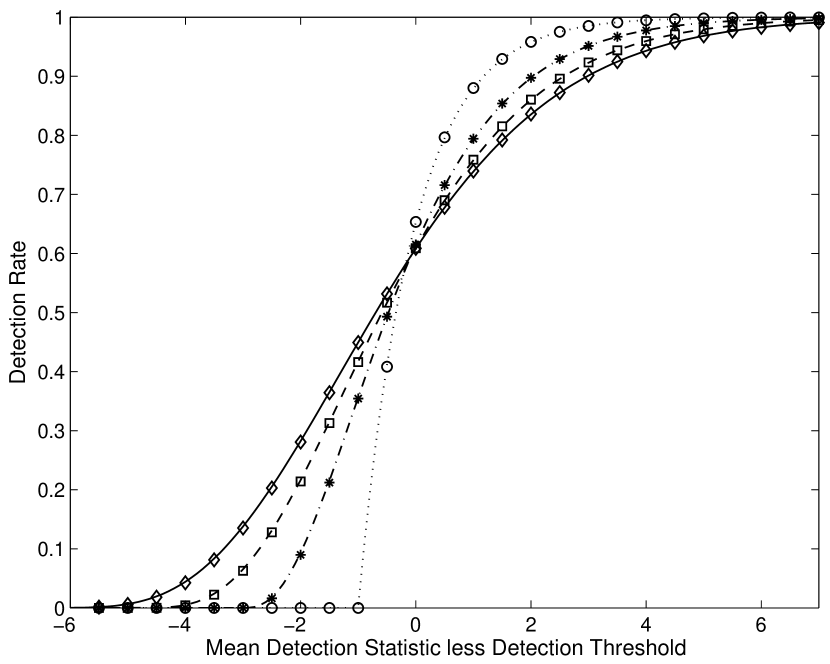
Figure 6: The detection rate as a function of the signal strength above the detection threshold (various symbols) along with analytic expressions (various curves) fitted to the empirical distributions. The number of assumed Fourier components, $M$=1, 3, 5 and 7, are denoted by circles, asterisks, squares and diamonds, respectively for the sample distributions. The corresponding analytical fits are denoted by dotted, dash-dotted, dashed and solid curves, respectively. For clarity, only every 5th point is plotted for the sample distributions. At the threshold, the detection rate attains $\sim$60%. This is due to the asymmetry of the distribution of null statistics. On this scale, the empirical distribution functions and the analytic expressions appear identical.

Table 1: Modeled Number of Main-Sequence Stars in Kepler’s Field of View

	Spectral Type
$m_{R}$	B5	A5	F5	G5	K5	M5	All
9.5	151	299	200	86	20	0	756
10.5	481	838	706	358	80	0	2463
11.5	1002	2181	2248	1300	242	7	6979
12.5	1832	5004	7037	4189	991	46	19098
13.5	3051	10245	19796	13379	3271	167	49909
14.5	4498	18142	51098	42035	10969	611	127352
Total	11014	36708	81085	61347	15573	831	206558

Table 2: Expected Number of Close-in Extrasolar Giant Planets (CEGPs) in Kepler’s Field of View

	Spectral Type
$m_{R}$	B5	A5	F5	G5	K5	M5	All
9.5	1	3	2	1	0	0	7
10.5	4	7	6	3	1	0	22
11.5	9	19	20	11	2	0	61
12.5	16	44	62	37	9	0	167
13.5	27	90	173	117	29	1	437
14.5	39	159	447	368	96	5	1114
Total	96	321	709	537	136	7	1807

Table 3: Expected Transiting CEGPs in Kepler’s Field of View

	Spectral Type
$m_{R}$	B5	A5	F5	G5	K5	M5	All
9.5	0	0	0	0	0	0	1
10.5	0	1	1	0	0	0	2
11.5	1	2	2	1	0	0	6
12.5	2	4	6	4	1	0	17
13.5	3	9	17	12	3	0	44
14.5	4	16	45	37	10	1	111
Total	10	32	71	54	14	1	181

Table 4: Number of Expected Detections vs. Assumed Number of Fourier Components

	Atmospheric Model
$M$	$\bar{r}=1.0$	$\bar{r}=0.1$	$p=2/3$	$p=0.15$	Average
1	173.7	168.7	738.0	158.9	309.8
2	184.7	155.3	736.6	146.9	305.9
3	183.8	140.4	719.7	130.8	293.7
4	175.0	126.7	706.6	117.6	281.5
5	165.8	116.1	693.6	107.7	270.8
6	159.1	108.6	683.2	101.0	263.0
7	152.9	102.5	675.6	96.0	256.8

Table 5: Analytical Fits to Monte Carlo Null Distributions

	Fit to Single Test				Fit to
	Direct Fit		Fit to Tail		Single Search
$M$	$A$	$B$	$A$	$B$	$N_{\mathrm{EIT}}$	Threshold
1	2.110	2.114	1.923	2.691	451.81	16.9
2	2.106	4.231	1.936	4.911	429.73	18.8
3	2.104	6.346	2.001	6.738	462.57	20.0
4	2.104	8.460	1.995	9.002	463.56	21.3
5	2.103	10.574	2.006	11.082	469.40	22.3
6	2.103	12.688	1.980	13.548	459.68	23.5
7	2.104	14.801	2.037	15.170	476.03	24.1

Table 6: Average Detection Rate for 1.2 R_J planets Orbiting Sun-Like Stars, (%)

	Apparent Stellar Magnitude
Prot	($m_{R}$)
(Days)	9.5	10.5	11.5	12.5	13.5	14.5
$\bar{r}$=1.0 $\mu$m Particles
5	0.0	0.0	0.0	0.0	0.0	0.0
10	0.0	0.0	0.0	0.0	0.0	0.0
15	0.0	0.0	0.0	0.0	0.0	0.0
20	12.2	12.0	11.8	10.8	8.2	2.6
25	36.0	35.7	34.6	31.8	24.0	8.2
30	49.6	48.7	47.4	43.5	33.2	13.3
35	59.3	58.2	55.3	53.0	40.8	15.9
40	66.5	65.9	64.4	56.6	44.6	16.8
$\bar{r}$=0.1 $\mu$m Particles
5	0.0	0.0	0.0	0.0	0.0	0.0
10	0.0	0.0	0.0	0.0	0.0	0.0
15	0.0	0.0	0.0	0.0	0.0	0.0
20	10.8	10.6	10.3	9.9	5.1	0.0
25	36.5	36.3	35.7	34.0	25.8	5.0
30	53.5	53.2	51.6	48.3	39.2	9.5
35	62.9	62.1	60.4	58.2	46.9	10.0
40	72.0	71.5	68.8	64.4	51.1	10.2
Albedo $p=0.15$ Lambert Sphere
5	0.0	0.0	0.0	0.0	0.0	0.0
10	0.0	0.0	0.0	0.0	0.0	0.0
15	0.0	0.0	0.0	0.0	0.0	0.0
20	6.8	6.7	6.3	4.9	1.0	0.0
25	38.6	38.4	37.5	34.0	25.4	1.2
30	56.6	56.4	55.9	52.7	42.4	4.6
35	67.3	67.1	65.6	61.2	50.0	5.6
40	75.6	75.4	74.4	70.1	54.7	5.9
Albedo $p=2/3$ Lambert Sphere
5	0.0	0.0	0.0	0.0	0.0	0.0
10	0.0	0.0	0.0	0.0	0.0	0.0
15	39.0	39.0	39.0	38.9	38.8	37.5
20	67.1	67.1	67.0	66.9	66.3	64.3
25	82.4	82.4	82.4	82.3	81.9	78.8
30	84.1	84.1	84.1	84.1	83.6	80.9
35	93.9	93.9	93.8	93.4	92.4	84.6
40	97.3	97.3	97.2	96.4	95.6	89.1

Table 7: Number of CEGPs Detected, Signal Adjusted for Stellar Radius

	Spectral Type
$m_{R}$	B5	A5	F5	G5	K5	M5	All
$\bar{r}$=1.0 $\mu$m Particles
9.5	0	0	0	0	0	0	1
10.5	0	0	0	1	1	0	2
11.5	0	0	0	5	2	0	7
12.5	0	0	1	14	7	0	23
13.5	0	0	2	37	22	1	62
14.5	0	0	0	54	60	5	120
Total	0	0	3	112	91	7	214
$\bar{r}$=0.1 $\mu$m Particles
9.5	0	0	0	0	0	0	1
10.5	0	0	0	1	1	0	2
11.5	0	0	0	5	2	0	7
12.5	0	0	1	16	7	0	24
13.5	0	0	2	42	23	1	68
14.5	0	0	0	50	64	5	119
Total	0	0	3	115	96	7	222
Lambert Sphere, $p$=0.15
9.5	0	0	0	0	0	0	1
10.5	0	0	0	2	1	0	2
11.5	0	0	0	5	2	0	8
12.5	0	0	1	17	7	0	25
13.5	0	0	1	46	22	1	71
14.5	0	0	0	45	60	5	110
Total	0	0	3	115	92	7	216
Lambert Sphere, $p$=2/3
9.5	0	0	0	1	0	0	1
10.5	0	0	1	3	1	0	4
11.5	0	0	4	9	2	0	15
12.5	0	0	13	29	8	0	50
13.5	0	0	38	93	27	1	160
14.5	0	0	104	283	90	5	482
Total	0	0	160	417	128	7	712

Table 8: Number of CEGPs Detected, Signal Not Adjusted for Stellar Radius

	Spectral Type
$m_{R}$	B5	A5	F5	G5	K5	M5	All
$\bar{r}$=1.0 $\mu$m Particles
9.5	0	0	0	0	0	0	0
10.5	0	0	0	1	0	0	2
11.5	0	0	1	4	1	0	6
12.5	0	0	2	13	3	0	19
13.5	0	0	6	32	9	1	48
14.5	0	0	6	40	11	1	59
Total	0	0	16	91	25	2	133
$\bar{r}$=0.1 $\mu$m Particles
9.5	0	0	0	0	0	0	0
10.5	0	0	0	1	0	0	2
11.5	0	0	1	5	1	0	6
12.5	0	0	3	14	4	0	21
13.5	0	0	5	36	10	1	52
14.5	0	0	3	24	7	1	34
Total	0	0	12	81	22	2	116
Lambert Sphere, $p$=0.15
9.5	0	0	0	0	0	0	0
10.5	0	0	0	1	0	0	2
11.5	0	0	1	5	1	0	7
12.5	0	0	2	15	4	0	21
13.5	0	0	4	38	10	1	53
14.5	0	0	1	13	3	0	18
Total	0	0	8	72	19	1	102
Lambert Sphere, $p$=2/3
9.5	0	0	1	1	0	0	1
10.5	0	0	2	2	1	0	5
11.5	0	0	6	9	2	0	16
12.5	0	0	19	28	7	0	55
13.5	0	0	58	89	24	1	173
14.5	0	0	161	272	76	5	514
Total	0	0	247	400	110	6	764

Table 9: Number of Background Binaries Not Excluded by Astrometry

	Apparent Stellar Magnitude
	($m_{R}$)
Parameter	9.5	10.5	11.5	12.5	13.5	14.5
Number of Background Binaries in Target Apertures	3	18	85	296	903	2405
Centroid Rejection Radius (arcsec)	$<$0.5	$<$0.5	$<$0.5	$<$0.5	$<$0.5	0.7
Aperture Size (square arcsec)	400	384	352	288	240	192
Number of Potential False Alarms	0	0	0	1	3	18

References

- Albrow et al. (2001) Albrow, M. D., Gilliland, R. L., Brown, T. M., Edmonds, P. D., Guhathakurta, P., Sarajedini, A. 2001, ApJ, 559, 1060
- Andersen et al. (1998) Andersen, B., Leifsen, T., Appourchaux, T., Frohlich, C., Jiménez, A., Wehrli, C. 1998, in Proceedings of the SOHO 6/GONG 98 Workshop, Structure and Dynamics of the Interior of the Sun and Sun-like Stars (Boston), 83
- Andersen (1996) Andersen, B. 1996, A&A, 312, 610
- Appourchaux et al. (2000) Appourchaux, T. & 14 other authors 2000, ApJ, 538, 401
- Baliunas & Vaughan (1985) Baliunas, S. L., Vaughan, A. 1985, Ann Rev Astron Ap, 23
- Bartolini et al. (1983) Bartolini, C., & 15 other authors 1983, A&A117, 149
- Batalha et al. (2002) Batalha, N., M., Jenkins, J., Basri, G. S., Borucki, W. J., & Koch, D. G. 2002, in Proceedings of the First Eddington Workshop, Stellar Structure and Habitable Planet Finding, ed. B. Battrick et al.(Cordoba: Noordwijk), 35
- Borucki et al. (1997) Borucki, W. J., Koch, D. G., Dunham, E. W., & Jenkins, J. M. 1997, in ASP Conf. Ser. 119, Planets Beyond the Solar System and The Next Generation of Space Missions, ed. D. Soderblom (San Francisco: ASP), 153
- Borucki et al. (1996) Borucki, W. J., Jenkins, J. M., Scargle, J., Koch, D., & Doyle, L. R. 1996, BAAS 28, 1115.
- Butler et al. (1999) Butler, R. P., Marcy, G. W., Fischer, D. A., Brown, T. M., Contos, A. R., Korzennik, S. G., Nisenson, P., Noyes, R. W. 1999, ApJ, 526, 916
- Cameron et al. (1999) Cameron, A. C., Horne, K., Penny, A., & James, D. 1999, Nature, 402, 751
- Charbonneau et al. (2002) Charbonneau, D., Brown, T. M., Noyes, R. W., Gilliland, R. L. 2002, ApJ, 568, 377
- Chugainov (1973) Chugainov, P. F. 1973, Izv Krym Astrofiz Obs, 48, 3
- Charbonneau et al. (1999) Charbonneau, D., Noyes, R. W., Korzennik, S. G., Nisenson, P., Jha, S., Vogt, S. S., & Kibrick, R. I. 1999, ApJ, 522, L145
- Cochran et al. (1997) Cochran, W. D., Hatzes, A. P., Butler, R. P., & Marcy, G. W. 1997, ApJ, 483, 457
- Cody & Sasselov (2002) Cody, A. M., Sasselov, D. D. 2002, ApJ, 569, 451
- Cram & Kuhi (1989) Cram, L. E., & Kuhi, L. V. 1989, FGK Stars and T Tauri Stars, NASA SP-502, (Washington, DC: US Gov. Printing Office)
- Deubner (1984) Deubner, F.-L., & Gough, G. O. 1984, Ann Rev Astron Ap, 22, 593
- Doyle (1996) Doyle, L. R., 1996, Photometric Spinoffs from the Kepler (Formerly FRESIP) Mission, SETI Institute whitepaper, March 27
- Duquennoy & Mayor (1991) Duquennoy, A., & Mayor, M. 1991, A&A, 248, 485
- Fröhlich et al. (1997) Fröhlich, C., et al.1997, SoPh, 175, 267
- Frölich (1987) Frölich, C., 1987, JGR, 92, 796
- Gray (1992) Gray, D. F., 1992, The Observation and Analysis of Stellar Photospheres (2nd edition; Cambridge: Cambridge Univ. Press)
- Green et al. (2002) Green, D., Mathews, J., & Seager, S. 2002, Presented at the Scientific Frontiers Conference in Research on Extrasolar Planets, Carnegie Institution, June 18-21
- Haywood, Robin, & Crézé (1997a) Haywood, M., Robin, A. C. & Crézé , M. 1997, A&A, 320, 420
- Haywood, Robin, & Crézé (1997b) Haywood, M., Robin, A. C. & Crézé , M. 1997, A&A, 320, 428
- Hudson (1988) Hudson, H. S., 1988, Ann Rev Astron Ap, 26, 473
- Jenkins (2002) Jenkins, J. M. 2002, ApJ, 575, 493
- Jenkins et al. (2002) Jenkins, J. M. , Caldwell, D. A., & Borucki, W. J. 2002, ApJ, 564, 495
- Jenkins et al. (2000b) Jenkins, J. M., Witteborn, F., Koch, D. G., Dunham, E. W., Borucki, W. J., Updike, T. F., Skinner, M. A. & Jordan, S. P. 2000, Proc. SPIE, 4013, 520
- Kawaler (1989) Kawaler, S. D. 1989, ApJ, 353, 65
- Kay (1998) Kay, S. 1998, Fundamentals of Statistical Signal Processing: Detection Theory, (Upper Saddle River: Prentice-Hall PTR)
- Knollenberg et al. (1980) Knollenberg, R. G., & Hunten, D. M. 1980, JGR, 85, 8036
- Kozhevnikov & Kozhevnikova (2000) Kozhevnikov, V. P. and Kozhevnikova, A. V. 2000, IBVS, 5252
- Koch et al. (2000) Koch, D. G., Borucki, W. J., Dunham, E. W., Jenkins, J. M., Webster, L., & Witteborn, F. 2000, Proc. SPIE, 4013, 508
- Lacy (1977) Lacy, C. H., ApJ, 218, 444
- Loeb & Gaudi (2003) Loeb, A., & Gaudi, B. S. 2003, astro-ph/0303212
- Mayor & Queloz et al. (1995) Mayor, M., & Queloz, D. 1995, Nature, 378, 355
- Messina et al. (2001) Messina, S., Rodono, M., & Guinan, E. F. 2001, A&A, 366, 215
- Noyes et al. (1984) Noyes, R. W., Hartmann, L., Baliunas, S. L., Dunkan, D. K., & Vaughan, A. H. 1984, ApJ, 279, 763
- Papoulis (1984) Papoulis, A. 1984, Probability, Random Variables, and Stochastic Processes, (New York: McGraw Hill)
- Perryman (2000) Perryman, M. A. C., 2000, Reports on Progress in Physics, 63, 1209
- Rabello-Soares et al. (1997) Rabello-Soares, M. C., Roca Cortes, T., Jimenez, A., Andersen, B. N., Appourchaux, T. 1997, A&A, 318, 970
- Radick et al. (1998) Radick, R. R., Lockwood, G. W., Skiff, B. A., & Baliunas, S. L. 1998, ApJS, 118, 239
- Remund et al. (2001) Remund, Q. P., Jordan, S. P., Updike, T. F., Jenkins, J. M., & Borucki, W. J. 2001, Proc. SPIE, 4495, 182
- Robin & Crézé (1986) Robin, A. C., & Crézé, M. 1986, A&A, 157, 71
- Rodonó et al. (1986) Rodonó, M., et al.1986, A&A, 165, 135
- Schneider et al. (1998) Schneider, J., et al.1998, in Origins, ASP Conf. Ser. 148, San Francisco, 298
- Seager et al. (2000) Seager, S., Whitney, B. A., & Sasselov, S. S. 2000, ApJ, 540, 505
- Sterken, & Jaschek (1996) Sterken, C., & Jaschek, C. 1996, Light Curves of Variable Stars (Cambridge U. Press, Cambridge)
- Walden et al. (1998) Walden, A. T., Percival, D. B., & McCoy, E. J. 1998, IEEE Trans Sig Proc, 46, 3153
- West et al. (1986) West, R. A., Stobel, D. F., & Tomasko, M. G., 1986, Icarus, 65, 161
- Willson & Hudson (1991) Willson, R. C. & Hudson, H. S. 1991, Nature, 351, 42