Small-scale CMB Temperature and Polarization Anisotropies Due to Patchy Reionization

Abstract

We study contributions from inhomogeneous (patchy) reionization to arcminute scale ($1000<\ell<10,000$) cosmic microwave background (CMB) anisotropies. We show that inhomogeneities in the ionization fraction, rather than in the mean density, dominate both the temperature and the polarization power spectra. Depending on the ionization history and the clustering bias of the ionizing sources, we find that rms temperature fluctuations range from 2 $\mu$K to 8 $\mu$K and the corresponding values for polarization are over two orders of magnitude smaller. Reionization can significantly bias cosmological parameter estimates and degrade gravitational lensing potential reconstruction from temperature maps but not from polarization maps. We demonstrate that a simple modeling of the reionization temperature power spectrum may be sufficient to remove the parameter bias. The high-$\ell$ temperature power spectrum will contain some limited information about the sources of reionization.

1 Introduction

Free electrons in the reionized (or reionizing) intergalactic medium (IGM) with peculiar velocities lead to new anisotropies as the CMB photons scatter off of them. Here we revisit predictions for the temperature and polarization power spectra of these new anisotropies at small angular scales in light of recent indications from observations by the Wilkinson Microwave Anisotropy Probe (WMAP) for an extended period of reionization (Kogut et al., 2003).

The argument for an extended period of reionization is as follows. The WMAP has detected the correlation between temperature and polarization on large angular scales (Kogut et al., 2003) that has an amplitude proportional to the total optical depth of CMB photons to Thomson scattering, $\tau$ (Sunyaev & Zeldovich, 1980; Zaldarriaga, 1997; Kaplinghat et al., 2002). Modeling reionization with a single sharp transition at $z_{ri}$, a multi–parameter fit to the WMAP data gives $z_{ri}=17\pm 5$ (Spergel et al., 2003). On the other hand, the evolution of quasar spectra from $z=6.3$ and $z=6.4$ to $z=6$ shows a rapid decrease in the amount of neutral Hydrogen, indicating the end of reionization (Fan et al., 2003). A simple interpretation to explain these two very different datasets is that reionization started early, $z_{ri}\sim 20$, but did not conclude until much later ($z\sim 6$).

As detected by WMAP, free electrons in the IGM scatter CMB photons and produce large angular scale CMB polarization. The fluctuations in the electron density field lead to small angular scale signatures both in the temperature and polarization. In the case of temperature, the new small scale anisotropy contribution is generally known as the kinetic Sunyaev-Zel’dovich (kSZ) effect (Sunyaev & Zeldovich, 1980) Inhomogeneities in the electron density may be due to perturbations in the baryon density or ionization fraction. If the ionized fraction is taken to be homogeneous and baryon density perturbations are calculated to first order then the effect is called the Ostriker-Vishniac (OV) effect (Ostriker & Vishniac, 1986; Vishniac, 1987). Non-linear effects from density perturbations make additional contributions beyond the OV effect on small scales (Hu, 2000; Gnedin & Jaffe, 2001; Ma & Fry, 2002). When only modulations in the ionized fraction are considered then we refer to the resulting temperature power spectrum as the patchy power spectrum. We focus on the patchiness because we find that, for the models we consider, variations in the ionized fraction are much more important than variations in the baryon density. For a review of the imprint of reionization on the CMB see Haiman & Knox (1999).

This extended period of reionization may be one in which the ionization fraction is highly inhomogeneous, i.e.“patchy”. As discussed by Aghanim et al. (1996), Gruzinov & Hu (1998) and Knox et al. (1998) (hereafter K98) such patchy reionization can lead to much larger anisotropies than homogeneous reionization (see also Valageas et al. 2001, Aghanim et al. 2002). Aghanim et al. (1996) and Gruzinov & Hu (1998) modeled the patches as spatially uncorrelated. K98 considered a model of correlated patches, and showed that these correlations were very important because they can greatly increase the signal in the $\ell=1000$ to 3000 range. In this paper we will take into account the correlations between these reionized patches by assuming they are associated with ionizing sources residing in dark matter halos. The correlations will then be proportional to the linear theory dark matter correlations, with the proportionality constant given by an average of the halo bias weighted by halo mass and an ionizing photon production efficiency factor, since these determine the size of the individual ionized patch around each dark halo. In our models, the kSZ power spectrum typically increases by an order of magnitude when the inhomogeneities in the ionized fraction are taken into account.

Patchy reionization also boosts the creation of polarization anisotropies on small angular scales. K98 pointed out that this polarization signal, since it is sourced by the temperature quadrupole as opposed to the velocities which have grown by gravitational instability, would be much smaller than the temperature signal. This was subsequently confirmed by explicit calculation (Weller, 1999; Hu, 2000). Hu (2000) pointed out that the B–mode power spectrum would be equal to the E–mode power spectrum (for a flat-sky version, see Baumann et al. 2002). We also calculate the polarization power spectrum from reionization and find that it is indeed too small to significantly affect cosmological parameter determination or lensing potential reconstruction.

Our paper is organized as follows. In § 2 we describe the kinetic SZ effect and how to calculate the temperature and polarization angular power spectra in the presence of ionization fraction and baryon density fluctuations. In § 3 we briefly describe our models for reionization (described with more detail in Haiman & Holder 2003), including our calculation of the effective bias of the patches. In § 4 we discuss the resulting power spectra and how they can be used as probes of reionization. We also derive in § 4.1 the expected errors from a ground–based experiment capable of detecting this signal. In § 5 we calculate the resulting bias in the cosmological parameter determination from Planck data that can be caused by patchy reionization, and show how simple phenomenological modeling can eliminate these biases. Finally, in § 6, we discuss the impact on lensing potential reconstruction. We conclude with a summary in § 7. Throughout the paper, unless stated otherwise, we will assume the cosmological parameters, $\Omega_{m}=0.29$, $\Omega_{\Lambda}=0.71$, $\Omega_{b}=0.047$, $h=0.72$, $\tau=0.17$ and $n=1$ with normalization $\sigma_{8}=0.9$ in agreement with a recent analysis of CMB data (Spergel et al., 2003).

2 Kinetic SZ effect

Compton-scattering via moving electrons leads to a Doppler effect and a corresponding temperature perturbation along the line-of-sight:

$$\frac{\Delta T}{T}({\bf\hat{n}})=\int d\eta\,a(\eta)\,g({\bf x},\eta)\,{\bf\hat{n}}\cdot{\bf v}\,,$$ (1)

where ${\bf\hat{n}}$ is the unit vector along the direction of observation, $\eta$ is the conformal time (with value $\eta_{0}$ today), ${\bf x}={\bf\hat{n}}(\eta_{0}-\eta)$ and ${\bf v}$ is the electron velocity. The visibility function, $g({\bf x},\eta)$, corresponds to the probability that the photon scattered at time $\eta$ and traveled freely since then:

$$g({\bf x},\eta)=\sigma_{T}\,n_{e}({\bf x},\eta)\,e^{-\tau(\eta)},$$ (2)

where $\tau$ is the optical depth to electron scattering between here and distance $\eta_{0}-\eta$ and $\sigma_{T}$ is the Thomson cross section. The free electron density is $n_{e}=X_{e}({\bf x},\eta)n_{p}({\bf x},\eta)$ and both the ionization fraction, $X_{e}$ and proton density, $n_{p}$, are allowed to have a spatial dependence.

Under a smooth distribution of free electrons with $n_{e}=\bar{n}_{e}$, the Doppler contribution to temperature anisotropies is significantly reduced as photons scatter against the crests and troughs of the velocity perturbations (Kaiser, 1984). This cancellation is avoided when there are significant fluctuations in the free electron density field, which can originate from perturbations in the ionized fraction ($\delta_{X_{e}}$) or the baryon density ($\delta_{b}$). The total contribution to the temperature anisotropy, up to second order, can then be expressed as:

$$\frac{\Delta T}{T}({\bf\hat{n}})=\sigma_{T}\,\bar{n}_{p}(\eta_{0})\int d\eta\,\left[a^{-2}(\eta)e^{-\tau}\bar{X}_{e}(\eta)\right]\,\,{\bf\hat{n}}\cdot{\bf q}\,,$$ (3)

with

$${\bf q}=(1+\delta_{X_{e}}+\delta_{b})\,{\bf v}$$ (4)

and $\sigma_{T}\,\bar{n}_{p}(\eta_{0})=2.03\times 10^{-5}\,\Omega_{b}h^{2}\,{\rm Mpc}^{-1}$.

2.1 Power spectrum

We next calculate the kSZ power spectrum on small angular scales, where the signal is not overwhelmed by the primary anisotropies. Then, for $\ell\gg 1$, we can use the Limber approximation (Limber, 1954) and write the spherical Fourier coefficient $C_{\ell}$ in terms of the 3D power spectrum of ${\bf q}({\bf x},\eta)$ (Kaiser, 1992; Dodelson & Jubas, 1995; Hu & White, 1996; Jaffe & Kamionkowski, 1998):

$$C_{\ell}=\sigma_{T}^{2}\,\bar{n}_{p}(\eta_{0})^{2}\int{d\eta\over x^{2}}\,a^{-4}(\eta)e^{-2\tau}\bar{X}_{e}^{2}(\eta)\,P_{q_{\perp}}\left({\ell\over x},\eta\right),$$ (5)

where

$$\langle{\bf q}_{\perp}({\bf k})\cdot{\bf q}_{\perp}^{*}({\bf k}^{\prime})\rangle=2(2\pi)^{3}\delta({\bf k}-{\bf k}^{\prime})\,P_{q_{\perp}}(k)$$ (6)

and ${\bf q}_{\perp}({\bf k})$ is the component of the 3D Fourier transform of ${\bf q}({\bf x})$ that is perpendicular to ${\bf k}$ (${\bf q}_{\perp}({\bf k})\cdot{\bf k}=0$). The implicit assumption here is that the quantity $\left[a^{-2}(\eta)e^{-\tau}\bar{X}_{e}(\eta)\right]$ is slowly-varying across a wavelength of the perturbation ($\Delta\eta\sim\eta_{0}/\ell$ at most). This is a good approximation for the angular scales of interest ($\ell\;\hbox to0.0pt{\lower 2.5pt\hbox{$\sim$}\hss}\raise 1.5pt\hbox{$>$}\;1000$).

The key quantity to compute is therefore $P_{q_{\perp}}$ for all possible contributions. To first order ${\bf q}={\bf v}$ and ${\bf v}({\bf k})\propto{\bf k}$ so that, as already stated, there will be no contribution to the CMB power spectrum from equation (5). At larger angular scales, on the other hand, the anisotropy from the component of ${\bf q}({\bf k})$ parallel to ${\bf k}$ becomes significant and is taken into account in standard Boltzmann calculations. Considering the density–modulated and ionized–fraction–modulated anisotropies, the components of ${\bf q}({\bf k})$ perpendicular to ${\bf k}$ are

$$q_{\perp,i}({\bf k}) = -i\int{d^{3}k^{\prime}\over(2\pi)^{3}}V({\bf k}^{\prime})\left({k_{i}^{\prime}\over k^{\prime}}-\mu^{\prime}{k_{i}\over k}\right)\times$$

$$\left[\delta_{b}(|{\bf k}-{\bf k}^{\prime}|)+\delta_{X_{e}}(|{\bf k}-{\bf k}^{\prime}|)\right],$$

where $\mu^{\prime}\equiv\hat{{\bf k}}\cdot\hat{{\bf k}}^{\prime}$ and we have assumed that the velocity field is a potential flow, ${\bf v}({\bf k})=-iV({\bf k})\hat{{\bf k}}$, as expected in linear perturbation theory. The corresponding power spectrum is then

$$P_{q_{\perp}}(k) = {1\over 2}\sum_{a,b=\delta_{b},\delta_{X_{e}}}\int{d^{3}k^{\prime}\over(2\pi)^{3}}\left[{\over}(1-\mu^{\prime 2})P_{ab}(|{\bf k}-{\bf k}^{\prime}|)P_{vv}(k^{\prime})\right.$$ (8)

$$-\left.{(1-\mu^{\prime 2})k^{\prime}\over|{\bf k}-{\bf k}^{\prime}|}P_{av}(|{\bf k}-{\bf k}^{\prime}|)P_{bv}(k^{\prime})\right].$$

Note that, due to geometric reasons, there is no connected fourth moment contribution to $P_{q_{\perp}}(k)$ (Cooray, 2001; Ma & Fry, 2002).

2.2 Density-modulated anisotropies

If reionization was homogeneous throughout the Universe, temperature anisotropies can only arise from perturbations in the baryon density (e.g. $a=b=\delta_{b}$ in equation 8). When $\delta_{b}$ is in the linear regime, this is the Ostriker-Vishniac effect (Ostriker & Vishniac, 1986; Vishniac, 1987), which has already been studied in some detail (Dodelson & Jubas, 1995; Hu et al., 1994; Persi et al., 1995; Hu & White, 1996; Jaffe & Kamionkowski, 1998; Hu, 2000). Here we will just try to give an order of magnitude estimate for the effect. For wavelengths that are much smaller than the coherence scale of the velocity fields, equation (8) simplifies considerably. First we note that, using the continuity equation:

$$P_{vv}(k^{\prime},\eta)\propto P_{\delta_{c}\delta_{c}}(k^{\prime})/k^{\prime 2}\,\,\,\,\,P_{\delta_{c}v}(k^{\prime},\eta)\propto P_{\delta_{c}\delta_{c}}(k^{\prime})/k^{\prime},$$

where we have assumed that the baryonic gas traces the cold dark matter. For large $k^{\prime}$, typically larger than $k_{m}\sim 0.1\ h/$Mpc (Hu, 2000) we then have $P_{vv}\sim 0$ and $P_{\delta_{c}v}\sim 0$ (density fluctuations uncorrelated with the bulk velocity field). Therefore, for large $k$ the integral in equation (8) can be evaluated under the approximation $|{\bf k}-{\bf k}^{\prime}|\approx k$ so that,

$$P_{q_{\perp}}(k,\eta)\sim{1\over 3}P_{\delta_{c}\delta_{c}}(k,\eta)v_{rms}^{2}(\eta),$$ (9)

with

$$v_{rms}^{2}=\int{k^{2}dk\over 2\pi^{2}}P_{vv}(k,\eta).$$ (10)

The factor of 1/3 arises from angular averaging, since only the line of sight component of the velocity field contributes to the signal (the two transverse parts drop out). For these small wavelengths, typically $P_{\delta_{c}\delta_{c}}(k)\propto k^{-3}$ so that, introducing the above expression in equation (5), gives $C_{\ell}\propto\ell^{-3}$ (for $\ell\gg\eta_{0}\,k_{m}$). Moreover, assuming our LCDM fiducial model and instantaneous reionization of the Universe, we obtain, as an order of magnitude estimate, $\ell^{2}C_{\ell}/(2\pi)\sim 3\times 10^{-13}(5000/\ell)$.

In the low redshift universe most of the baryonic matter resides in collapsed, high density objects. We therefore need to modify the above expressions to take into account the non-linearities of the density perturbations (Hu, 2000; Gnedin & Jaffe, 2001; Ma & Fry, 2002). These non-linearities only affect the density field below the coherence scale of the bulk velocity. Therefore, equation (9) will be a good approximation for scales that become non-linear. One then only needs to obtain the corresponding non-linear matter power spectrum using an appropriate prescription such as the halo model (Ma & Fry, 2000). Figure 1 compares the OV power spectrum with the non-linear correction calculated using the halo model (thin lines). We see that for sufficiently large $\ell$ there is an increase in power due to a similar increase in the matter power spectrum. We point out that this non–linear OV effect includes contributions to the kSZ signal from low redshift galaxy clusters. As will be seen below, the amplitude of the kSZ signal from the high–redshift ionized patches overwhelms this low–redshift contribution in most reionization models. The results in Ma & Fry (2002) agree reasonably well with hydrodynamical simulations (Springel et al., 2001; da Silva et al., 2001; White et al., 2002) for the angular scales of interest.

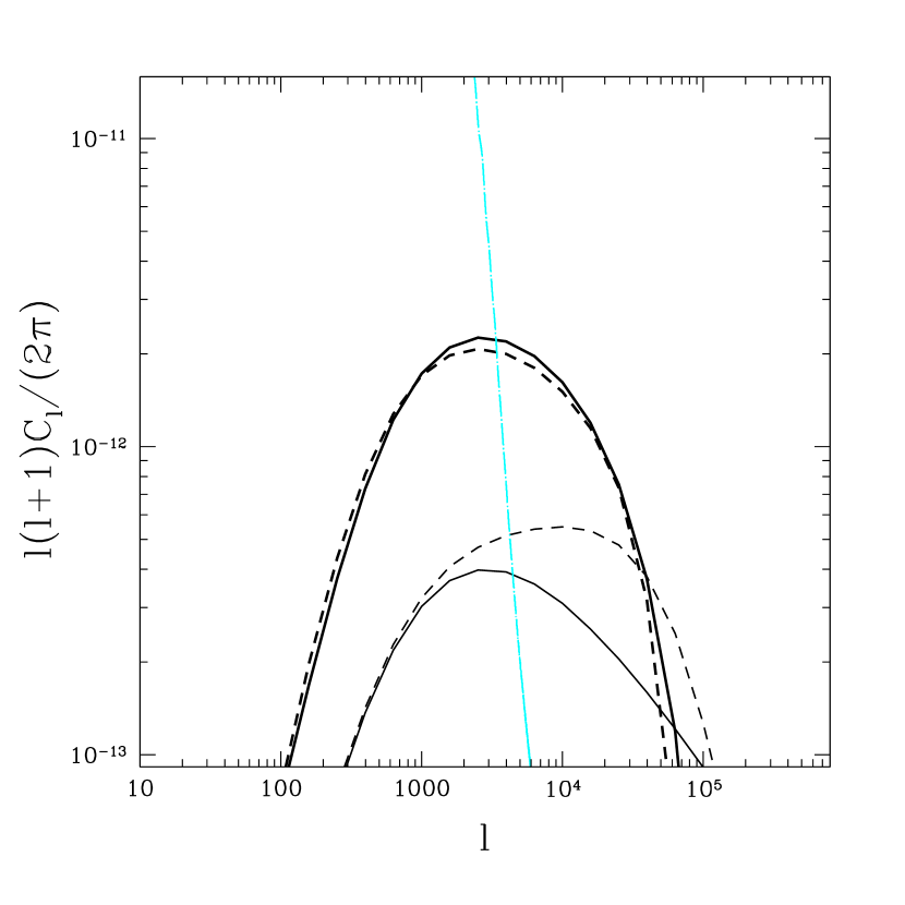
Figure 1: The several contributions to the kSZ temperature power spectrum assuming the LCDM model described in the introduction. The thin solid line is the O-V power spectrum from homogeneous reionization and dashed line is the non-linear correction. The thick solid line is the typical contribution from inhomogeneous reionization and uses the model shown in Figure 3 and 4 (solid line). Dashed line shows the approximate model from eq. (17). The patchy power spectrum basically follows the shape of the matter power spectrum. Also shown is the primary lensed CMB power spectrum (dot-dashed).

2.3 Patchy reionization

Exactly as with perturbations in the matter density, inhomogeneities in the ionized fraction create temperature anisotropies through modulation of the Doppler effect (K98, Gruzinov & Hu 1998). Considering the case where $a=b=\delta_{X_{e}}$ in equation (8), we now need to obtain an expression for $P_{{\delta_{X_{e}}}{\delta_{X_{e}}}}(k)$. We assume the ionizing radiation is coming from stars formed from gas clouds that cooled in dark matter halos. The dark halo correlation function can be expressed in terms of the linear theory dark matter one (Mo & White, 1996; Jing, 1998):

$$\xi_{halo}(r;M,M^{\prime},\eta)=b(M,\eta)b(M^{\prime},\eta)\xi_{\delta_{c}\delta_{c}}(r,\eta),$$ (11)

where $\xi_{halo}(r;M,M^{\prime})$ is the correlation function between halos of mass $M$ and $M^{\prime}$ and $b()$ is the clustering bias parameter. To obtain the clustering properties of the ionized fraction we need to take into account the dependence of the size and spatial distribution of the ionizing patches on the masses and ionization efficiencies of dark halos. Therefore, one should be able to write the correlation as:

$$\xi_{{\delta_{X_{e}}}{\delta_{X_{e}}}}(r,\eta)=b^{2}_{eff}(\eta)\xi_{\delta_{c}\delta_{c}}(r,\eta)$$ (12)

where $b_{eff}$ is the mean bias weighted by the different halo properties. Since these ionizing patches are rare objects we expect them to be more clustered than the underlying dark matter (e.g. $b_{eff}>1$). We will compute this bias in more detail in Section 3. Finally, one has to take into account that the perturbations will be smoothed out on scales smaller than the size of the patch. Choosing a Gaussian filter, the power spectrum for the ionized fraction will then be

$$P_{{\delta_{X_{e}}}{\delta_{X_{e}}}}(k,\eta)=b^{2}_{eff}(\eta)P_{\delta_{c}\delta_{c}}(k,\eta)e^{-k^{2}R^{2}},$$ (13)

where $R$ is the mean radius of the ionized patches (HII regions).

We crudely model the time–dependence of $R$ as

$$R\sim\left({1\over 1-\bar{X}_{e}}\right)^{1/3}R_{p},$$ (14)

where $R_{p}$ is the (comoving) size of the fundamental patch which we take to be $R_{p}\sim 100$  Kpc. The cutoff scale $R$ is equal to $R_{p}$ when reionization starts and increases with time as HII regions overlap and form larger HII regions. Equation 14 follows from assuming a Poisson distribution of patches and that their volumes add when they overlap. But the essential consequence of equation (14) is that on the scales of interest ($\ell\lesssim 10,000$ or $R\gtrsim 1$Mpc) the transition is very sudden; i.e., $R$ increases from 1 Mpc to $\infty$ very rapidly. We expect this behavior to be generic and thus our results should be insensitive to the specifics of the overlap modeling.

To calculate the patchy power spectrum we neglect the cross–correlation between velocity and $\delta_{X_{e}}$ since it is small, though we discuss this contribution later. Then, we simply plug expression (13) into equation (8). The result for our fiducial reionization model (discussed in the next section) is shown in Figure 1. To have a better understanding of the expected shape and amplitude of this power spectrum we will now derive an approximate expression. Using an expression similar to equation (9) we find the patchy power spectrum to be

$$C_{\ell}={\sigma_{T}^{2}\,\bar{n}_{p}(\eta_{0})^{2}\over 3} \int_{\eta_{i}}^{\eta_{1}}{d\eta\over x^{2}}\,a^{-4}(\eta)e^{-2\tau}\bar{X}_{e}^{2}(\eta)\times$$ (15)

$$P_{{\delta_{X_{e}}}{\delta_{X_{e}}}}\left({\ell\over x},\eta\right)v_{rms}^{2}(\eta),$$

where $\eta_{i}$ signals the start of reionization (when $X_{e}$ starts increasing from its value at recombination) and $\eta_{1}$ corresponds to the time when $\bar{X}_{e}=1$. We can write the time dependence of the dark matter perturbation as $\delta_{c}(k,\eta)\ =\ \left({G\over G_{0}}\right)\delta_{c}(k,\eta_{0})$, where $G$ is the growth factor (Carroll et al., 1992) and $G_{0}$ is the value today. Moreover, assuming $x_{i}-x_{1}\ll x_{1}$, we can pull the $\ell$ dependence out of the time integration, so that:

$$C_{\ell} \approx {\sigma_{T}^{2}\,\bar{n}_{p}^{2}\over 3\bar{x}^{2}}P_{\delta_{c}\delta_{c}}\left({\ell\over\bar{x}}\right)e^{-{\ell^{2}\bar{R}^{2}\over\bar{x}^{2}}}\left({v_{rms}(\eta_{0})\over G_{0}\dot{G}_{0}}\right)^{2}\times$$ (16)

$$e^{-2\bar{\tau}}\int_{\eta_{i}}^{\eta_{1}}d\eta\,a^{-2}\bar{X}_{e}^{2}(\eta)\,b_{eff}^{2}(\eta)(G\dot{G})^{2},$$

where $\dot{G}\equiv{dG\over d\eta}$. The quantities, $x$, $R$ and $\tau$ are assumed to be evaluated at the average time, $(\eta_{1}+\eta_{i})/2$. At the redshifts of interest for the above time integration, the cosmological constant is negligible, so that $G\sim a$ and $H\sim H_{0}\sqrt{\Omega_{m}/a^{3}}$. The power spectrum can then be expressed as

$$\ell^{2}C_{\ell}/(2\pi) \sim 6.18\times 10^{-21}\ell^{3}\,T^{2}(\ell/\bar{x})e^{-{\ell^{2}\bar{R}^{2}\over\bar{x}^{2}}}\times$$ (17)

$$\int_{z_{1}}^{z_{i}}{dz\over\sqrt{1+z}}\bar{X}_{e}^{2}(z)\,b_{eff}^{2}(z),$$

where we are using our fiducial cosmological model, so that $v_{rms}(\eta_{0})/c=1.8\times 10^{-3}$, $\bar{x}\sim 8.0\times 10^{3}$ Mpc/h and $\bar{R}\sim 0.20$ Mpc/h. The matter power spectrum is normalized to give $\sigma_{8}=0.9$ and the transfer function, $T(k)$ (Bardeen et al., 1986; Eisenstein & Hu, 1998; Seljak & Zaldarriaga, 1996), is normalized to 1 on large scales. All the dependence on the reionization model is in the time integration, through $\bar{X}_{e}$ and $b_{eff}$. Therefore we expect the power spectrum from different reionization histories to have approximately the same shape but different amplitudes. Figure 1 shows a possible power spectrum from the above patchy reionization model. Also shown is the approximate model from equation (17). This signal typically overwhelms the OV effect, even when including the non-linear correction, which can be traced back to the large effective bias, $b_{eff}\;\hbox to0.0pt{\lower 2.5pt\hbox{$\sim$}\hss}\raise 1.5pt\hbox{$>$}\;5$, in equation (16).

We have ignored the term, $\langle v_{1}{\delta_{X_{e}}}_{2}\rangle\langle v_{2}{\delta_{X_{e}}}_{1}\rangle$ as sub-dominant to $\langle{\delta_{X_{e}}}_{1}{\delta_{X_{e}}}_{2}\rangle\langle v_{1}v_{2}\rangle$. The former term may become important for length scales above the velocity coherence length, which projects to $l\sim 500$ from high redshifts. Due to the tendency of overdense regions to fall toward each other, this term is negative and the net effect will be a suppression of power. This power suppression will be small in the scales of interest. We have also neglected the cross correlation $\langle\delta_{c}{\delta_{X_{e}}}\rangle$ because it will be suppressed by approximately one factor of the bias from $\langle{\delta_{X_{e}}}{\delta_{X_{e}}}\rangle$.

2.4 Polarization Signatures

Thomson scattering of radiation with a quadrupole anisotropy generates linear polarization in the CMB. Again, the dominant source at small angles is the modulation of the quadrupole through perturbations in the matter density or ionized fraction. The power spectra of the $E$ and $B$ parity states are then (Hu, 2000; Baumann et al., 2002)

$$C_{\ell}^{EE} = C_{\ell}^{BB}={3\sigma_{T}^{2}\,\bar{n}_{p}(\eta_{0})^{2}\over 100}\int{d\eta\over x^{2}}\,a^{-4}(\eta)e^{-2\tau}\bar{X}_{e}^{2}(\eta)\times$$ (18)

$$\left(P_{\delta_{c}\delta_{c}}+P_{\delta_{X_{e}}\delta_{X_{e}}}\right)\,Q_{rms}^{2}(\eta),$$

where $Q_{rms}$ is the quadrupole anisotropy. The power spectrum from the primordial quadrupole source will typically dominate over the kinematic and intrinsic contributions (Hu, 2000). Moreover, this quadrupole is a slowly varying function of time and can be taken out of the integral above. Figure 2 shows the patchy and density contributions to polarization (using $Q_{rms}\sim 25\mu$K), compared to the $B$ mode polarization from tensor and lensing effects. Again the patchy signal dominates over the density modulated polarization. However, it does not seem to be an important contaminant on the relatively large scales ($\ell\;\hbox to0.0pt{\lower 2.5pt\hbox{$\sim$}\hss}\raise 1.5pt\hbox{$<$}\;200$) where tensor $B$ modes are significant, and it is well below the scalar $E$ mode on all scales.

The patchy polarization power spectrum is $\sim 10^{5}$ times smaller than the patchy temperature power spectrum because $Q_{\rm rms}\sim 10^{-2}v_{\rm rms}$ and due to the geometric factor of 100 in equation 18 in place of the factor of 3 in equation 15.

Figure 2: $B$ mode polarization for our fiducial model, with contributions from lensing (thin solid line) and tensor modes (thin-dashed) with a tensor to scalar ratio of $10^{-3}$. Also shown is the contribution from density (thick dashed) and ionization (thick solid) modulated scattering. The density modulated contribution assumes gas traces dark matter and uses the halo model for non-linear corrections. Also shown for comparison is the scalar E mode contribution (dot-dashed line).

3 Reionization Models

We now need to obtain the evolution of the electron fraction, $\bar{X}_{e}$ and effective bias, $b_{eff}$, in physically motivated models of the reionization history. For that purpose, we adapt semi–analytical models from Haiman & Holder (2003), modified to include the spatial biasing of the ionizing sources and hence of the ionized regions. These models fit all the relevant observations (including the electron scattering optical depth $\tau=0.17$ measured by WMAP and inferences from redshift $z\sim 6$ quasar spectra). For details, the reader is referred to that paper; here we provide only a brief summary, and a description of how the bias is calculated.

We follow the volume filling fractions $F_{\rm HII}$ of HII regions (which, by definition, equals the mean electron fraction $\bar{X}_{e}$) assuming that discrete ionized Strömgren spheres are being driven into the IGM by ionizing sources located in dark matter halos. In this picture, each fluid element is engulfed by an ionization front at a different time. Reionization has a complex history that reflects contributions from three distinct types of ionizing sources, and two different feedback effects (all of which have physical motivations as described in detail in Haiman & Holder 2003). In short, ionizing sources (assumed to be massive metal–free stars) first appear inside gas that cools via ${\rm H_{2}}$ lines, and collects in the earliest non–linear halos with virial temperature of $100\,{\rm K}\;\hbox to0.0pt{\lower 2.5pt\hbox{$\sim$}\hss}\raise 1.5pt\hbox{$<$}\;T\;\hbox to0.0pt{\lower 2.5pt\hbox{$\sim$}\hss}\raise 1.5pt\hbox{$<$}\;10^{4}$K (Haiman et al., 1996). These sources ionize $\sim 50\%$ of the volume in hydrogen. However, at this stage (redshift $z\sim 17$) the entire population of these sources effectively shuts off due to global ${\rm H_{2}}$–photodissociation by the cosmic soft UV background they had built up (Haiman et al., 1997a, b, 2000). Soon more massive halos, with virial temperatures of $10^{4}\,{\rm K}\;\hbox to0.0pt{\lower 2.5pt\hbox{$\sim$}\hss}\raise 1.5pt\hbox{$<$}\;T\;\hbox to0.0pt{\lower 2.5pt\hbox{$\sim$}\hss}\raise 1.5pt\hbox{$<$}\;2\times 10^{5}$K form, which do not rely on ${\rm H_{2}}$ to cool their gas (they cool via neutral H excitations), and new ionizing sources turn on in these halos. These are assumed to be “normal” stars, since the gas had already been enriched by heavy elements from the first generation. This population continues ionizing hydrogen, but is also self–limiting: gas infall to these relative shallow potential wells is prohibited inside regions that had already been ionized and photo–heated to $10^{4}$K (Thoul & Weinberg, 1996). As a result, hydrogen reionization starts slowing down around $z\sim 10$. However, at this stage, still larger halos with virial temperatures of $T\;\hbox to0.0pt{\lower 2.5pt\hbox{$\sim$}\hss}\raise 1.5pt\hbox{$>$}\;2\times 10^{5}$K start forming. These relatively massive halos are impervious to photoionization feedback, and complete the reionization of hydrogen at around $z\approx 7$.

In order to predict the kSZ signal, we need to compute in our models the mean bias of the ionized regions as a function of redshift. At any given redshift, there is an ensemble of HII regions, the sum of which make up the total ionized volume fraction. Each HII region has at least one ionizing source, each of which has a fixed halo mass and formation redshift.

We assume that the volume of each ionized region scales linearly with halo mass within each of three distinct mass bins; we only allow a dependence of ionizing photon production efficiencies in discrete jumps between these bins. This assumption could be relaxed to include more generic dependencies on halo mass. This, in general, would change the effective bias we obtain, but would involve introducing more free parameters; we avoid this complication in the present paper. Under these assumptions, the mean bias of ionized regions can be computed as follows. We first note that at a given redshift, the total volume–filling fraction $F_{\rm HII}$ is given by

$$F_{\rm HII} (z)=\rho_{\rm b}(z)\int_{\infty}^{z}dz^{\prime}\left\{\epsilon_{\rm Ib}\frac{dF_{\rm coll,Ib}}{dz}(z^{\prime})+\left[1-F_{\rm HII}(z^{\prime})\right]\right.\times$$ (19)

$$\left.\left[\epsilon_{\rm Ia}\frac{dF_{\rm coll,Ia}}{dz}(z^{\prime})+\epsilon_{\rm II}\frac{dF_{\rm coll,II}}{dz}(z^{\prime})\right]\right\}{\tilde{V}}_{\rm HII}(z^{\prime},z),$$

where $\rho_{\rm b}=\Omega_{\rm b}\rho_{\rm crit}$ is the average baryonic density and $\rho_{\rm crit}$ is the critical density of the universe. In the second term on the right hand side of equation (19), we have explicitly included a factor $(1-F_{\rm HII})$, which takes into account the photoionization feedback. Here $F_{\rm coll,II}$, $F_{\rm coll,Ia}$ and $F_{\rm coll,Ib}$, are the fractions of baryons collapsed into halos of increasing mass ranges. For example (using $\bar{\rho}_{\rm tot}$ as the present–day total mass density),

$$F_{\rm coll,II}\equiv{1\over\bar{\rho}_{\rm tot}}\int_{M_{\rm min}}^{M_{\rm max}}dM\frac{dn}{dM}(z)M$$ (20)

where $M_{\rm min}$ and $M_{\rm max}$ correspond to halo virial temperatures of $T_{\rm vir}=100$K and $T_{\rm vir}=10^{4}$K at redshift $z$, respectively. The $\epsilon_{\rm II}$, $\epsilon_{\rm Ia}$ and $\epsilon_{\rm Ib}$ are the efficiencies in these halos of producing and leaking ionizing photons into the IGM. The efficiencies are defined as the product $\epsilon_{*}\equiv N_{\gamma}f_{*}f_{\rm esc}$, where $f_{*}\equiv M_{*}/(\Omega_{\rm b}M_{\rm halo}/\Omega_{m})$ is the fraction of baryons in the halo that turns into stars; $N_{\gamma}$ is the mean number of ionizing photons produced by an atom cycled through stars, averaged over the initial mass function (IMF) of the stars; and $f_{\rm esc}$ is the fraction of these ionizing photons that escapes into the IGM. Finally, ${\tilde{V}}_{\rm HII}(z_{\rm on},z)$ is the volume per unit mass and unit efficiency ionized by redshift $z$ by a single source that turned on the earlier redshift $z_{\rm on}>z$. The evolution of $F_{\rm HII}$ for a few models described in Haiman & Holder (2003) is shown in Figure 3. They all produce a total electron scattering optical depth of $\tau=0.17$ by construction, in agreement with the WMAP result. For the one we take as our fiducial model in this paper (solid line), the efficiencies are $\epsilon_{\rm II}=200$ and $\epsilon_{\rm Ia}=\epsilon_{\rm Ib}=80$.

Figure 3: $\bar{X}_{e}$ for three different fiducial models with $\tau=0.17$. Solid line is for the fiducial model used throughout the paper. Dashed line assumes that $H_{2}$ feedback effectively shuts off star formation in all Type II halos. Dot-dashed line assumes that a transition from metal free to normal star formation takes place abruptly at a certain redshift.

To calculate the effective clustering bias for any field, the first step is to write the field as an integral over halo mass and formation redshifts, which we have effectively done with equation (19) and (20). We then use this sum to define $b_{eff}$ as the appropriate weighted average of the bias factor for a halo of mass $M$ and formation redshift $z$, $b(z,M)$. The effective bias for the ionization fraction for our reionization models can thus be efficiently written as:

$$b_{eff}(z)=F^{b}_{\rm HII}/F_{\rm HII}$$ (21)

where

$$F^{b}_{\rm HII} (z)\equiv\rho_{\rm b}(z)\int_{\infty}^{z}dz^{\prime}\biggl{\{}\epsilon_{\rm Ib}b_{\rm Ib}(z^{\prime})\frac{dF_{\rm coll,Ib}}{dz}(z^{\prime})+$$ (22)

$$\left[\epsilon_{\rm Ia}b_{\rm Ia}(z^{\prime})\frac{dF_{\rm coll,Ia}}{dz}(z^{\prime})+\epsilon_{\rm II}b_{\rm II}(z^{\prime})\frac{dF_{\rm coll,II}}{dz}(z^{\prime})\right]\times$$

$$\left[1-F_{\rm HII}(z^{\prime})\right]\biggr{\}}{\tilde{V}}_{\rm HII}(z^{\prime},z)$$

and

$$b_{\rm II}(z)\equiv\left[F_{\rm coll,II}\,\bar{\rho}_{\rm tot}\right]^{-1}\int_{M_{\rm min}}^{M_{\rm max}}dM\frac{dn}{dM}(z)b(z,M)M,$$ (23)

with analogous expressions defining $b_{\rm Ia}(z)$ and $b_{\rm Ib}(z)$.

In this last equation, $b(z,M)$ is the usual halo bias (Mo & White 1996). The averaging over formation redshift only introduces a small correction to the bias calculation, since at a given redshift most of the contribution comes from young ionizing sources.

Figure 4 shows the effective bias for the same three models as in Figure 3. The increase of the bias as $z$ decreases toward $\sim 7$ is due to the formation of rare, massive halos, which play an important role in the last stages of reionization.

Note that the bias factor as calculated in Eq. (21), Eq. (22) and (23) agrees with the halo model description of source bias (Cooray & Sheth, 2002) when one makes the connection between the presence of ionized electrons and the halo occupation distribution. Here, the bias factors are calculated with the assumption that ionized electrons occupy halos with mass in the range $M_{\rm min}$ and $M_{\rm max}$, such that the mean halo occupation number is unity in this mass range and zero otherwise.

Figure 4: Effective bias (equation 21) for the same fiducial models as in Figure 3.

We now remark on the robustness of the model of patchy reionization we have presented. This simple picture has the HII regions localized around the halos hosting the ionizing sources. Further, our calculation of $V(z,z^{\prime})$ assumes the recombination rate is given by the square of the background density times some constant clumping factor. In reality, there must be complicated shapes for the volume $V(z,z^{\prime})$, which depend on the three-dimensional arrangement of the density field, and also on the locations and strengths of the ionizing sources. The degree of localization of the HII regions around the sources of ionizing photons will also depend on how hard the radiation is, with harder spectra reionizing more uniformly (Oh et al., 2001; Venkatesan et al., 2001). And, if reionization is from decaying dark matter then $X_{e}$ would be yet more uniform (Hansen & Haiman, 2003).

Another simple, but complementary, picture (Miralda-Escudé et al., 2000) (hereafter MHR) is that the ionizing radiation from a source leaves the surrounding dense regions neutral and the i-fronts propagate along directions of the the lowest column density into the voids. In this case it actually does not matter that the sources are in high-$\sigma$ peaks. MHR postulate that all gas below some threshold density, $\rho_{t}$, is ionized, and all gas above this $\rho_{t}$ remains neutral. The patchy power spectrum in this case could be computed using the two-point function of regions with $\rho<\rho_{t}$.

The MHR picture is the extreme opposite of ours (see also Peebles & Juszkiewicz 1998). Which picture is a better description of reality depends entirely on how rapidly percolation occurs. We assume it only happens as $\bar{X}_{e}$ gets very close to unity. For our calculations to be correct at $l\lesssim 10,000$ requires that prior to $\bar{X}_{e}\sim 1$, the ionizing radiation in the HII regions mostly comes from sources closer than 3 Mpc.

4 Temperature Power Spectra

In Figure 5, we plot the patchy power spectrum for the three reionization models (including our fiducial model), all with the same cosmological parameters and $\tau=0.17$ but differing $X_{e}(z)$ and $b_{\rm eff}(z)$. As expected, the shapes are very similar. Allowing $\tau$ to vary also does not significantly affect the shape, as demonstrated by the fourth model plotted with $\tau=0.11$ but higher bias that is close to a $\tau=0.17$ model. The higher bias is achieved by moving the ionizing sources to more massive halos (Type Ia and Ib). The optical depth is prevented from dropping even further by increasing the efficiencies in Type Ia halos.

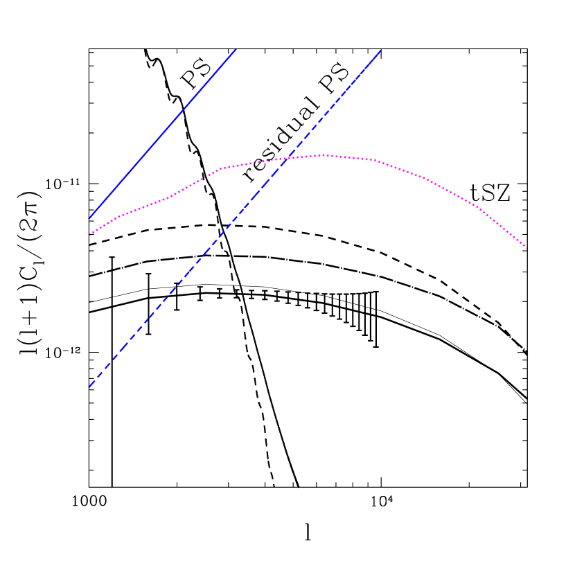
Figure 5: Patchy power spectra for the reionization models in Figure 3 (same line styles), together with other astrophysical contributions and expected measurement errors (see text). The solid (dashed) straight line is the the point source contribution at 217 GHz before (after) multi-frequency cleaning. The primary unlensed (dashed) and lensed (solid) CMB power spectra are also shown as is the thermal SZ power spectrum from White et al. (2002) (dotted) with its expected amplitude at lower frequencies. The thin line close to the solid one shows the patchy power spectrum for a model with $\tau=0.11$ but large bias.

The degeneracy between $\tau$ and bias means that $\tau$ cannot be inferred from the kSZ power spectrum alone, as suggested by Zhang et al. (2003). However, if $\tau$ becomes tightly constrained by polarization measurements at low $\ell$, which is possible with future missions (Holder et al., 2003), the mean effective bias for the sources of reionization can be determined. Having this information will constrain the typical halo masses of the sources that dominate reionization. Whether the sources are located in the 2-sigma or in the 3-sigma peaks is important for the physics of reionization (see Rees 1999). This will also constrain the mean efficiency $\epsilon$.

To demonstrate the range of possible power spectrum amplitudes we calculate the patchy power spectra for a variety of reionization models with values of $\tau$ spanning the 2$\sigma$ range allowed by WMAP. In Figure 6 we plot the patchy power spectrum with variations in $\tau$ about two of the models shown in Figure 5 (solid and dashed lines). Variations in $\tau$ for the solid (dashed) line are done by essentially changing the efficiencies in the Type II (Ia) halos. Again the shape is very similar (at least up to $\ell\sim 10^{4}$) with the amplitudes ranging from $1\times 10^{-12}$ to $8\times 10^{-12}$ at $\ell\sim 2000$.

At $\ell>10^{4}$ the power spectrum is sensitive to the structure of the reionized patches on comoving length scales smaller than 1 Mpc. At these smaller scales the details of the patch geometries and sizes become important. With sufficiently reliable modeling of the power spectrum on these scales (which we have not attempted) observations at $l>10^{4}$ could be used to constrain these patch properties, although contamination by point sources will make such observations difficult.

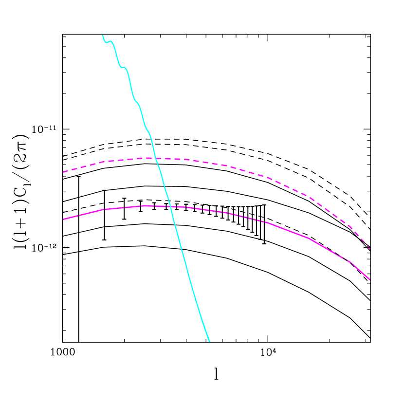
Figure 6: Patchy power spectrum for variations in $\tau$ about two of the models shown in Figure 5 (thick solid and dashed lines). Solid lines correspond to the following values of $\tau$ (from bottom to top): 0.05, 0.11, 0.17, 0.24, 0.31. Dashed lines correspond to $\tau=$0.11, 0.17, 0.22, 0.28. Also shown are the expected measurement errors and primary lensed CMB power spectrum.

4.1 Measuring the kSZ Power Spectrum

Ground-based observations, with 1^′ to 2^′ angular resolution, may be able to measure the kSZ power spectrum. In order to do so, several other astrophysical signals must be cleaned from the maps: namely, thermal SZ and emission from dusty galaxies.

We take as an illustrative example a multi-frequency experiment that includes a channel at 217 GHz. We assume that the thermal SZ in the 217 GHz channel is insignificant, or at least that the residuals after multi-frequency cleaning are insignificant. We further assume the 217 GHz channel has an angular resolution of $\theta_{b}=0^{\prime}.9$ and an rms error of $\Delta_{T}=12\mu$K on every beam-size pixel in a fraction, $f_{\rm sky}=0.01$, of the sky, or 400 sq. degrees.

For our point source model, we adopt model E of Guiderdoni et al. (1998). For this model, with 0^′.9 resolution, 10 mJy point sources stand out as 5$\sigma$ fluctuations where $\sigma^{2}$ is the variance due to sources fainter than 10 mJy. Removing these bright sources with a 5$\sigma$ cut leaves a power spectrum due to the faint point sources of $l^{2}C^{\rm ps}_{l}/(2\pi)=2.5\times 10^{-12}(l/2000)^{2}$ and is plotted as the solid straight line in Figure 5. Exploiting the frequency dependence of these remaining sources (with respect to CMB temperature fluctuations) might reduce the power in this contamination by a factor of 10 (dashed blue line).

The error on the total fluctuation power is

$$\Delta C_{l}^{\rm tot} = \sqrt{2\over(2l+1)f_{\rm sky}}(C_{l}^{\rm tot}+N_{l})\,{\rm where}$$

$$C_{l}^{\rm tot} = C_{l}^{\rm P}+C_{l}^{\rm PS}+C_{l}^{\rm kSZ}{\rm\ \ \ and}$$

$$N_{l} = (\Delta_{T}\theta_{b})^{2}\exp(l^{2}\theta_{b}^{2}/(8\ln{2})).$$ (24)

Here $C_{l}^{\rm P}$ corresponds to the primary anisotropy contribution and $C_{l}^{\rm kSZ}$ is the power spectrum from the kSZ effect. A multi-parameter fit to $C_{l}^{\rm kSZ}$, the amplitude of a shot-noise spectrum, and the cosmological parameters governing $C_{l}^{\rm P}$ will result in

$$\Delta C_{l}^{\rm kSZ}\approx\Delta C_{l}^{\rm tot}$$ (25)

since $C_{l}^{\rm P}$ and $C_{l}^{\rm PS}$ will be very well determined. We plot the $\Delta C_{l}^{\rm tot}$ errors in Figure 5 about our fiducial kSZ model.

5 Impact on Parameter Determination

The large anisotropies at $\ell\;\hbox to0.0pt{\lower 2.5pt\hbox{$\sim$}\hss}\raise 1.5pt\hbox{$>$}\;1000$ predicted from a patchy reionization phase may significantly affect the high precision parameter estimation predicted for future CMB experiments. Let us suppose we obtain a set of best fit parameters ${a_{i}}$ by minimizing the likelihood, $\mathcal{L}^{o}$, without considering the patchy reionization signal (e. g. ${\partial\ln{\mathcal{L}^{o}}\over\partial a_{i}}=0$). The above set should be shifted by an amount $\delta a_{i}$ so that they minimize the true likelihood, $\mathcal{L}^{n}$, which includes the patchy contribution:

$$\delta a_{i}=\sum_{j}\mathcal{F}_{ij}^{-1}{\partial\ln{\mathcal{L}^{n}}\over\partial a_{j}},$$ (26)

where $\mathcal{F}_{ii^{\prime}}$ is the fisher matrix,

$$\mathcal{F}_{ij}=-\langle{\partial^{2}\ln{\mathcal{L}^{n}}\over\partial a_{i}\partial a_{j}}\rangle.$$ (27)

The bias in the estimation of each parameter will then be, as in K98,

$$\delta a_{i}\approx-\sum_{j\ell}\mathcal{F}_{ij}^{-1}{C_{\ell}^{R}\over\sigma_{\ell}^{2}}{\partial C_{\ell}^{P}\over\partial a_{j}},$$ (28)

where $C_{\ell}^{R}$ can represent the power spectrum from inhomogeneous reionization and $\sigma_{\ell}$ is the error expected on the $C_{\ell}$’s, e.g. the sum of the errors due to sample variance and noise, $N_{\ell}$ (Knox, 1995; Bond et al., 1997; Zaldarriaga, 1997), $\sqrt{2\over 2\ell+1}(C_{\ell}^{P}+C_{\ell}^{R}+N_{\ell})$. We estimated the bias for the same set of cosmological parameters as in Kaplinghat et al. (2003) taking into account the weak lensing contribution on small scales. Using our fiducial model for $C_{\ell}^{R}$, Table 1 shows the expected bias for Planck (Tauber, 2001).

Table 1: Bias and standard deviation in the parameter estimation for Planck ($\ell_{\rm max}=3000$).

	$\Omega_{m}h^{2}$	$\Omega_{b}h^{2}$	$n_{s}$	$n_{s}^{\prime}$	$m_{\nu}$	$Y_{H_{e}}$	$z_{r}$	$\theta_{s}$	$\ln{P_{\Phi}}$	$w_{x}$
bias	0.00012	0.00025	-0.030	-0.022	-1.20	-0.10	1.9	-0.0006	0.03	0.74
$1\sigma$	0.0013	0.00030	0.013	0.0050	0.45	0.021	3.2	0.0026	0.048	0.56

In Figure 7 we plot the ratio of this systematic offset to the statistical uncertainty as a function of the maximum multipole considered.

Figure 7: Absolute ratio of bias to 1$\sigma$ for Planck as a function of $\ell_{max}$. Shown are the parameters that will have a significant bias: $n_{s}$ (continuous line), $m_{\nu}$ (dotted), $Y_{H_{e}}$ (dashed), $n_{s}^{\prime}$ (dot-dashed) and $w_{x}$ (long-dashed).

The situation is even worse for a sample variance dominated experiment. As we can see in Table 2, most of the biases are already important at $\ell=2000$, thus becoming a problem for parameter estimation.

Table 2: Bias and standard deviation in the parameter estimation for a sample variance dominated experiment ($\ell_{\rm max}=2000$)

	$\Omega_{m}h^{2}$	$\Omega_{b}h^{2}$	$n_{s}$	$n_{s}^{\prime}$	$m_{\nu}$	$Y_{H_{e}}$	$z_{r}$	$\theta_{s}$	$\ln{P_{\Phi}}$	$w_{x}$
bias	-0.00018	0.00030	-0.030	-0.0210	-1.14	-0.105	0.88	-0.00006	0.019	0.40
$1\sigma$	0.00100	0.00027	0.011	0.0049	0.43	0.018	2.87	0.0020	0.044	0.52

The solution is to obtain a model for the patchy power spectrum in terms of a few parameters and take them into account when doing a multi-dimensional fit to the data. Looking at equation (16) we see that although the amplitude depends on the reionization model, the shape does not. Let $C_{\ell}^{1}$ be a typical $C_{\ell}$ from patchy reionization, then any other reionization model can be written as $C_{\ell}^{f}\approx AC_{\ell}^{1}$. There will still be a bias due to the slight differences in shape between the reionization models (e.g. $C_{\ell}^{R}=C_{\ell}^{f}-AC_{\ell}^{1}$). Table 3 shows the ratio, ${\rm bias}/\sigma$, for a cosmic–variance dominated experiment when considering the amplitude as an extra parameter. We see that the expected bias is now negligible at the cost of an increase in the statistical uncertainty.

Table 3: Ratio of bias to statistical uncertainty.

	$\Omega_{m}h^{2}$	$\Omega_{b}h^{2}$	$n_{s}$	$n_{s}^{\prime}$	$m_{\nu}$	$Y_{H_{e}}$	$z_{r}$	$\theta_{s}$	$\ln{P_{\Phi}}$	$w_{x}$	A
${bias/\sigma_{n}}$	0.027	0.027	-0.060	-0.083	-0.030	-0.077	-0.008	-0.031	-0.008	0.007	0.011
${\sigma_{n}/\sigma_{o}}$	1.0	1.4	1.1	1.0	2.4	1.0	1.0	1.0	1.1	1.4

The dominant source of the increased statistical uncertainty is the remaining uncertainty in the amplitude of the patchy power spectrum. This uncertainty can be reduced by experiments sensitive to $l>3000$ where the patchy power spectrum dominates, such as considered in the previous Section.

6 Impact on Lensing Potential Reconstruction

To understand the secondary confusion related to patchy reionization in lensing reconstruction with CMB data, we follow suggested approaches in the literature (Hu & Okamoto, 2002; Cooray & Kesden, 2003) and modify the noise calculation related to lensing reconstruction to include the kSZ contribution. In the case of temperature, the variance of quadratic statistics, with $\hat{\Theta}^{2}({\bf l})$ as the filtered version of the squared temperature (see, for example, Cooray & Kesden 2003), leads to a reconstructed lensing potential power spectrum of

$$\langle\hat{\Theta}^{2}({\bf l})\hat{\Theta}^{2}({\bf l}^{\prime})\rangle=(2\pi)^{2}\delta_{D}({\bf l}+{\bf l}^{\prime})\left[C_{l}^{\phi\phi}+N_{l}^{\phi\phi}\right]\,,$$ (29)

where the noise is

$$[N_{l}^{\phi\phi}]^{-1}=\int\frac{d^{2}{\bf l}_{1}}{(2\pi)^{2}}\frac{[{\bf l}\cdot{\bf l}_{1}C_{l_{1}}^{P}+{\bf l}\cdot({\bf l}-{\bf l}_{1})C_{|{\bf l}-{\bf l}_{1}|}^{P}]^{2}}{2C_{l_{1}}^{\rm tot}C_{|{\bf l}-{\bf l}_{1}|}^{\rm tot}}\,.$$ (30)

Here, $C_{l}^{P}$ is the power spectrum of unlensed primordial temperature fluctuations, while, following equation (24), $C_{l}^{{\rm tot}}$ accounts for all contributions to the temperature power spectrum including noise. Instead of point sources included in equation (24), here, we include foreground contributions related to secondary effects, mainly thermal (tSZ) and kinetic (kSZ) SZ contributions.

In Figure 8, we summarize our results where we show the deflection angle power spectrum, $C_{l}^{dd}=l(l+1)C_{l}^{\phi\phi}$ and related noise contributions. In addition to temperature, we have also considered lensing reconstruction from polarization data and have concentrated on the quadratic combination related to E and B-mode maps. This combination provides the best estimator for lensing reconstruction from CMB data if the signal-to-noise is sufficiently high (Hu & Okamoto, 2002). In calculating these noise curves, we assume temperature and polarization maps with noise rms of 2 $\mu$K in each beam–size pixel, and a beam size of 3^′. Such sensitivities may be achieved by future ground or space-based missions.

The thermal SZ contribution boosts the noise by an order of magnitude from the case with noise alone. This is, however, not a significant source of worry since the SZ thermal contribution can be removed from thermal CMB maps based on the frequency spectrum of the SZ contribution in multifrequency data. The source of worry will then be the kSZ signal, including the contribution from patchy reionization. We show the level of expected noise following our calculation related to Figure 1. The noise is a factor of a few higher than the case of detector noise alone.

Equation (29) assumes that the patchy power spectrum is perfectly known. Uncertainties in the amplitude and shape will further increase the noise in the lensing potential reconstruction, though probably not by much since measurements at $l\sim 5000$ combined with modeling (such as described in our paper) can be used to constrain the amplitude and shape.

While the lensing reconstruction from temperature data is degraded, this is not the case for polarization. As shown in Figure 8, the noise level including patchy reionization is the same as when only detector noise is included. Even for a perfect polarization map with no detector noise, the reconstruction with polarization is not significantly affected since the level of foreground noise is significantly below the cosmic variance limit of the E-mode power and below the cosmic variance of lensed scalars in the B-mode power. Thus, polarization observations provide a confusion free way to extract lensing information and to study primordial anisotropy contributions.

In addition to foreground noise variance, given by their power spectra, the foreground secondary effects can also be correlated with lensing potentials. While this leads to an additional noise contribution, we have found this to be significantly smaller than the Gaussian noise shown in Fig. 1, since the quadratic maps are prefiltered to maximize lensing reconstruction such that other higher order correlations are reduced (Cooray & Kesden, 2003). Another secondary source of noise is the non-Gaussianity of foregrounds themselves. In the case of kSZ related to patchy reionization, we expect this contribution to be negligible since at high redshifts clustering is linear and on large scales we will be averaging over the contributions from many patches.

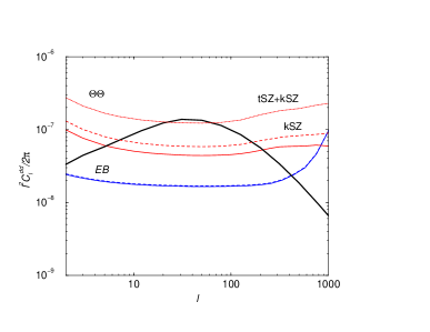
Figure 8: The deflection angle power spectrum (black thick solid line) and the noise variance for its reconstruction with different assumptions. In solid red, we show the noise related to reconstruction with temperature maps while in blue we show the same using polarization data (based on the quadratic combination of E mode with B mode). The dotted line shows the reconstruction noise with temperature in the presence of SZ thermal effect. This secondary contribution can be removed in multi frequency data using the SZ spectrum. The resulting lensing reconstruction is then affected by the kSZ signal from patchy reionization (red dashed line). The blue dashed line shows the same noise in the presence of kSZ polarization contribution. The latter is significantly smaller and leads to the same noise when the polarization from patchy reionization is ignored.

7 Summary

The kSZ power spectrum is important phenomenologically in two ways: 1) as a contaminant of the primary/lensing CMB power spectrum and 2) as an interesting probe of the epoch of reionization. We have shown that, if neglected, the patchy contribution can lead to statistically significant biases in the cosmological parameters estimated from Planck data. Higher–resolution observations (such as by ACT, APEX, SPT ) could be even more strongly affected. We have proposed a simple solution, which is to phenomenologically parameterize the patchy power spectrum. Fortunately for this purpose, as we have seen analytically, although the amplitude in the relevant l range is highly uncertain, the shapes are not. For the models we have considered, extending our cosmological parameter set to include one more parameter (the amplitude of the patchy power spectrum) eliminates any significant bias (even for an all-sky cosmic-variance limited experiment to $\ell=3000$).

In addition to parameter estimation, high–resolution temperature and polarization anisotropies are affected by gravitational lensing. CMB maps can be used to reconstruct the lensing potential, whose auto and cross power spectra (cross with CMB maps and cosmic shear lensing potential maps) are sensitive to the dark energy properties and neutrino masses. We have also investigated the degradation of lensing potential reconstruction and conclude that lensing studies with temperature data alone will be affected by fluctuations related to patchy reionization while polarization data will not be affected. Thus parameter estimation and lensing–potential reconstruction from polarization are much less affected by reionization than is the case for temperature anisotropies.

The kSZ power spectrum can also give us some information about the reionization process. At $l\gtrsim 3000$ and at frequencies near the null of the thermal SZ effect, the kSZ reionization power spectrum will be the dominant source of fluctuation power on the sky, after cleaning out point sources. SZ survey instruments such as ACT, SPT, APEX and CARMA with the ability to clean out the thermal SZ signal based on its spectral dependence will be able to make highly accurate measurements of the kSZ power spectrum. We have calculated the expected power spectrum errors for a nominal observation, including modeling of residual point source contamination. If $\tau$ becomes tightly constrained, this type of experiment should allow us to determine the mean effective bias and thus provide important information about the sources of reionization.

In this paper we have only calculated power spectra. We expect that these two-point functions are the most important statistics, both for consideration of patchy reionization as a signal and as a contaminant (see Castro 2003 for a discussion of non-Gaussianity from homogeneous reionization). At $\ell\lesssim 10^{4}$, we expect the signal to be approximately Gaussian due to the large number of patches along each line of sight. Non–Gaussian properties may also be of interest and have been studied by Gnedin & Shandarin (2002), though at very small scales ($\ell\sim 10^{5}$).

References

- Aghanim et al. (2002) Aghanim, N., Castro, P. G., Melchiorri, A., & Silk, J. 2002, A&A, 393, 381
- Aghanim et al. (1996) Aghanim, N., Desert, F. X., Puget, J. L., & Gispert, R. 1996, A&A, 311, 1
- Bardeen et al. (1986) Bardeen, J. M., Bond, J. R., Kaiser, N., & Szalay, A. S. 1986, ApJ, 304, 15
- Baumann et al. (2002) Baumann, D., Cooray, A., & Kamionkowski, M. 2002, ArXiv Astrophysics e-prints (New Astronomy, in press), 8511
- Bond et al. (1997) Bond, J. R., Efstathiou, G., & Tegmark, M. 1997, MNRAS, 291, L33
- Carroll et al. (1992) Carroll, S. M., Press, W. H., & Turner, E. L. 1992, ARA&A, 30, 499
- Castro (2003) Castro, P. G. 2003, Phys. Rev. D, 67, 123001
- Cooray (2001) Cooray, A. 2001, Phys. Rev. D, 64, 63514
- Cooray & Kesden (2003) Cooray, A., & Kesden, M. 2003, New Astronomy, 8, 231
- Cooray & Sheth (2002) Cooray, A., & Sheth, R. 2002, Phys. Rep., 372, 1
- da Silva et al. (2001) da Silva, A. C., Kay, S. T., Liddle, A. R., Thomas, P. A., Pearce, F. R., & Barbosa, D. 2001, ApJ, 561, L15
- Dodelson & Jubas (1995) Dodelson, S., & Jubas, J. M. 1995, ApJ, 439, 503
- Eisenstein & Hu (1998) Eisenstein, D. J., & Hu, W. 1998, ApJ, 496, 605
- Fan et al. (2003) Fan, X., Strauss, M. A., Schneider, D. P., Becker, R. H., White, R. L., Haiman, Z., Gregg, M., Pentericci, L., Grebel, E. K., Narayanan, V. K., Loh, Y., Richards, G. T., Gunn, J. E., Lupton, R. H., Knapp, G. R., Ivezić, Ž., Brandt, W. N., Collinge, M., Hao, L., Harbeck, D., Prada, F., Schaye, J., Strateva, I., Zakamska, N., Anderson, S., Brinkmann, J., Bahcall, N. A., Lamb, D. Q., Okamura, S., Szalay, A., & York, D. G. 2003, AJ, 125, 1649
- Gnedin & Jaffe (2001) Gnedin, N. Y., & Jaffe, A. H. 2001, ApJ, 551, 3
- Gnedin & Shandarin (2002) Gnedin, N. Y., & Shandarin, S. F. 2002, MNRAS, 337, 1435
- Gruzinov & Hu (1998) Gruzinov, A., & Hu, W. 1998, ApJ, 508, 435
- Guiderdoni et al. (1998) Guiderdoni, B., Hivon, E., Bouchet, F. R., & Maffei, B. 1998, MNRAS, 295, 877
- Haiman et al. (2000) Haiman, Z., Abel, T., & Rees, M. J. 2000, ApJ, 534, 11
- Haiman & Holder (2003) Haiman, Z., & Holder, G. P. 2003, ArXiv Astrophysics e-prints, 2403
- Haiman & Knox (1999) Haiman, Z., & Knox, L. 1999, in ASP Conf. Ser. 181: Microwave Foregrounds, 227
- Haiman et al. (1997a) Haiman, Z., Rees, M. J., & Loeb, A. 1997a, ApJ, 476, 458
- Haiman et al. (1997b) —. 1997b, ApJ, 484, 985
- Haiman et al. (1996) Haiman, Z., Thoul, A. A., & Loeb, A. 1996, ApJ, 464, 523
- Hansen & Haiman (2003) Hansen, S. H., & Haiman, Z. 2003, ArXiv Astrophysics e-prints, 5126
- Holder et al. (2003) Holder, G., Haiman, Z., Kaplinghat, M., & Knox, L. 2003, astro-ph/0302404
- Hu (2000) Hu, W. 2000, ApJ, 529, 12
- Hu & Okamoto (2002) Hu, W., & Okamoto, T. 2002, ApJ, 574, 566
- Hu et al. (1994) Hu, W., Scott, D., & Silk, J. 1994, Phys. Rev. D, 49, 648
- Hu & White (1996) Hu, W., & White, M. 1996, Astron. & Astrophys., 315, 33
- Jaffe & Kamionkowski (1998) Jaffe, A. H., & Kamionkowski, M. 1998, Phys. Rev. D, 58, 043001
- Jing (1998) Jing, Y. P. 1998, ApJ, 503, L9+
- Kaiser (1984) Kaiser, N. 1984, ApJ, 282, 374
- Kaiser (1992) —. 1992, ApJ, 388, 272
- Kaplinghat et al. (2003) Kaplinghat, M., Chu, M., Haiman, Z., Holder, G. P., Knox, L., & Skordis, C. 2003, ApJ, 583, 24
- Kaplinghat et al. (2002) Kaplinghat, M., Knox, L., & Skordis, C. 2002, ApJ, 578, 665, astro-ph/0203413
- Knox (1995) Knox, L. 1995, Phys. Rev. D, 52, 4307
- Knox et al. (1998) Knox, L., Scoccimarro, R. ., & Dodelson, S. 1998, Phys. Rev. Lett., 81, 2004
- Kogut et al. (2003) Kogut, A., et al. 2003, astro-ph/0302213
- Limber (1954) Limber, D. N. 1954, ApJ, 119, 655
- Ma & Fry (2000) Ma, C., & Fry, J. N. 2000, ApJ, 543, 503
- Ma & Fry (2002) —. 2002, Physical Review Letters, 88, 211301
- Miralda-Escudé et al. (2000) Miralda-Escudé, J., Haehnelt, M., & Rees, M. J. 2000, ApJ, 530, 1
- Mo & White (1996) Mo, H. J., & White, S. D. M. 1996, MNRAS, 282, 347
- Oh et al. (2001) Oh, S. P., Haiman, Z., & Rees, M. J. 2001, ApJ, 553, 73
- Ostriker & Vishniac (1986) Ostriker, J. P., & Vishniac, E. T. 1986, ApJ, 306, L51
- Peebles & Juszkiewicz (1998) Peebles, P. J. E., & Juszkiewicz, R. 1998, ApJ, 509, 483
- Persi et al. (1995) Persi, F. M., Spergel, D. N., Cen, R., & Ostriker, J. P. 1995, ApJ, 442, 1
- Rees (1999) Rees, M. J. 1999, ArXiv Astrophysics e-prints, 2345
- Seljak & Zaldarriaga (1996) Seljak, U., & Zaldarriaga, M. 1996, ApJ, 469, 437
- Spergel et al. (2003) Spergel, D. N., et al. 2003, astro-ph/0302209
- Springel et al. (2001) Springel, V., White, M., & Hernquist, L. 2001, ApJ, 549, 681
- Sunyaev & Zeldovich (1980) Sunyaev, R. A., & Zeldovich, I. B. 1980, MNRAS, 190, 413
- Tauber (2001) Tauber, J. A. 2001, in IAU Symposium, 493–+
- Thoul & Weinberg (1996) Thoul, A. A., & Weinberg, D. H. 1996, ApJ, 465, 608
- Valageas et al. (2001) Valageas, P., Balbi, A., & Silk, J. 2001, A&A, 367, 1
- Venkatesan et al. (2001) Venkatesan, A., Giroux, M. L., & Shull, J. M. 2001, ApJ, 563, 1
- Vishniac (1987) Vishniac, E. T. 1987, ApJ, 322, 597
- Weller (1999) Weller, J. 1999, ApJ, 527, L1
- White et al. (2002) White, M., Hernquist, L., & Springel, V. 2002, ApJ, 579, 16
- Zaldarriaga (1997) Zaldarriaga, M. 1997, Phys. Rev. D, 55, 1822
- Zhang et al. (2003) Zhang, P., Pen, U., & Trac, H. 2003, ArXiv Astrophysics e-prints, 4534