Gamma-Ray Bursts versus Quasars: Lyman-$\alpha$ Signatures of Reionization versus Cosmological Infall

Abstract

Lyman-$\alpha$ absorption is a prominent cosmological tool for probing both galactic halos and the intergalactic medium at high redshift. We consider a variety of sources that can be used as the Lyman-$\alpha$ emitters for this purpose. Among these sources, we argue that quasars are the best probes of the evolution of massive halos, while $\gamma$-ray bursts represent the cleanest sources for studying the reionization of the intergalactic medium.

1. Introduction

Over the past three decades, quasars have been traditionally used to probe the intervening intergalactic medium (IGM) at redshifts $z\lesssim 6$ when this medium was highly ionized. The polarization anisotropies of the microwave background measured by WMAP indicate that the IGM was significantly ionized at a much higher redshift $z\sim 17\pm 4$ (Spergel et al., 2003), possibly implying two separate reionization phases separated by a prolonged period of nearly complete recombination (Wyithe & Loeb, 2003a, b; Cen, 2003). Attention is now shifting towards direct observations of the epoch of reionization. The process of reionization started with the emergence of individual H II regions centered on discrete sources, which eventually overlapped [see reviews by Barkana & Loeb (2001); Loeb & Barkana (2001)]. Observationally, a central goal is to determine the average neutral fraction of the IGM, and possibly even map the topology of the H II islands, as a function of redshift. The main problem with using resonant Ly$\alpha$ absorption by neutral hydrogen for this purpose is that the corresponding resonant cross-section is too large; a neutral fraction as small as $\sim 10^{-3}$ is already sufficient to suppress the quasar flux below detectability. For example, the spectrum of the Sloan Digital Sky Survey (SDSS) quasar at $z=6.28$ shows complete absorption [the so-called Gunn-Peterson (1965) trough] of its spectral flux shortward of the Ly$\alpha$ resonance wavelength at the quasar redshift (Becker et al., 2001), but it remains unclear whether the IGM is highly ionized or whether it contains pockets of neutral gas at this redshift (Barkana, 2002; Fan et al., 2002).

The use of other atomic lines is problematic for other reasons. For example, absorption by metal lines (Oh, 2002) can only probe regions that had been previously metal-enriched by supernovae and the ionization state of this disturbed gas may not be representative of the entire IGM (since most metals may reside within H II bubbles near their source galaxies). Another possible probe, 21 cm absorption by neutral hydrogen, suffers from a cross-section that is too small (the opposite problem from Ly$\alpha$) leading to a very low optical depth and requiring the use of very bright radio sources ($\gtrsim 10$ mJy) that should be rare in the early universe (Carilli, Gnedin, & Owen, 2002; Furlanetto & Loeb, 2002). Detection of 21 cm absorption or emission against the microwave background is technologically challenging (Tozzi, Madau, Meiksin, & Rees, 2000; Iliev, Shapiro, Ferrara, & Martel, 2002; Furlanetto, Sokasian, & Hernquist, 2003) and is likely to be overwhelmed by foregrounds (Di Matteo, Perna, Abel, & Rees, 2002; Loeb, 1996).

It is therefore important to explore any possible way of using the Ly$\alpha$ absorption signature near the source in order to measure the IGM neutral fraction. In fact, for photon wavelengths longer than the Ly$\alpha$ resonance at the source redshift, the absorption cross-section is weaker (since these photons are offset from resonance) and so the quasar spectrum should gradually recover its unabsorbed spectral flux level as the wavelength becomes redder. The detailed spectral shape of the red damping wing of the Gunn-Peterson trough can potentially be used to infer the neutral hydrogen fraction in the IGM during the epoch of reionization. Miralda-Escudé (1998) calculated this shape for the idealized case of a weak point source embedded in a neutral uniformly expanding IGM. In reality, however, the ionizing effect of a quasar on the surrounding IGM [the so-called ”proximity effect” (Bajtlik, Duncan, & Ostriker, 1988)] complicates this interpretation (Cen & Haiman, 2000; Madau & Rees, 2000). In addition, cosmological infall changes the IGM density and velocity field near bright early quasars because these are likely to be hosted by a massive galaxy; Barkana & Loeb (2003) have shown that this effect can be used as an important tool in itself, as a way to measure directly the masses of the host dark matter halos of quasars, and to test fundamental aspects of the processes of galaxy and quasar formation. Indeed, we explore this tool further in this paper and consider how infall around quasars can be probed over a broad range of halo masses and redshifts.

Given that quasars and their massive hosts perturb the IGM around them both radiatively and gravitationally, the following question arises: Are there better sources than quasars for probing the Ly$\alpha$ damping wing during reionization? Our answer is positive. These sources are the afterglows of Gamma-Ray Bursts (GRBs), suggested before for this purpose (Miralda-Escudé, 1998; Loeb, 2003) but with additional advantages that we highlight in this paper.

GRBs are the brightest electromagnetic explosions in the universe, and should be detectable out to redshifts $z>10$ (Lamb & Reichart, 2000; Ciardi & Loeb, 2000). High-redshift GRBs can be easily identified through infrared photometry, based on the Ly$\alpha$ break induced by absorption of their spectrum at wavelengths below $1.216\,\mu{\rm m}\,[(1+z)/10]$. Follow-up spectroscopy of high-redshift candidates can then be performed on a 10-meter-class telescope. There are three main advantages of GRBs relative to quasars:

• The afterglow flux at a given observed time lag after the $\gamma$-ray trigger is not expected to fade significantly with increasing redshift, since higher redshifts translate to earlier times in the source frame, during which the afterglow is intrinsically brighter (Lamb & Reichart, 2000; Ciardi & Loeb, 2000). For standard afterglow lightcurves and spectra, the increase in the luminosity distance with redshift is compensated by this cosmic time-stretching effect.

• In the standard $\Lambda$CDM cosmology, galaxies form hierarchically, starting from small masses and increasing their average mass with cosmic time. Hence, the characteristic mass of quasar black holes and the total stellar mass of a galaxy were smaller at higher redshifts, making these sources intrinsically fainter (Wyithe & Loeb, 2002). However, GRBs are believed to originate from a stellar mass progenitor and so the intrinsic luminosity of their engine should not depend on the mass of their host galaxy. At high redshifts, a GRB should strongly dominate the luminosity of its host galaxy. Hence GRBs are expected to be increasingly brighter than any other competing source as higher redshifts are considered.

• Since the GRB progenitors are believed to be stellar, they likely originate in the most common star-forming galaxies at a given redshift rather than in the most massive host galaxies, as is the case for bright quasars. Low mass host galaxies induce only a weak ionization effect on the surrounding IGM and do not greatly perturb the Hubble flow around them. Hence, the Ly$\alpha$ damping wing should be closer to the idealized unperturbed IGM case (Miralda-Escudé, 1998) and its detailed spectral shape should be easier to interpret. Note also that unlike the case of a quasar, a GRB afterglow can itself ionize at most $\sim 4\times 10^{4}E_{51}M_{\odot}$ of hydrogen if its UV energy is $E_{51}$ in units of $10^{51}$ ergs, and so it should have a negligible cosmic effect on the surrounding IGM.

Although the nature of the central engine that powers the relativistic jets of GRBs is unknown, recent evidence indicates that GRBs trace the formation of massive stars (Bloom et al., 2002; Kulkarni et al., 2000; Totani, 1997; Wijers et al., 1998; Blain & Natarajan, 2000). Since the first stars are predicted to be predominantly massive (Abel, Bryan, & Norman, 2002; Bromm, Coppi, & Larson, 2002), their death might give rise to large numbers of GRBs at high redshifts. Detection of high-redshift GRBs could probe the earliest epochs of star formation, one massive star at a time. The upcoming Swift satellite (see http://swift.gsfc.nasa.gov/), scheduled for launch in May of 2004, is expected to detect about a hundred GRBs per year. Bromm & Loeb (2002) calculated the expected redshift distribution of GRBs; under the assumption that the GRB rate is simply proportional to the star formation rate they found that about a quarter of all GRBs detected by Swift should originate at $z>5$ (see also Lamb & Reichart, 2000). This estimate is rather uncertain because of the poorly determined GRB luminosity function. We caution further that in principle, the rate of high-redshift GRBs may be significantly suppressed if the early massive stars fail to launch a relativistic outflow. This is possible, since metal-free stars may experience negligible mass loss before exploding as a supernova. They would then retain their massive hydrogen envelope, and any relativistic jet might be quenched before escaping the star (Heger et al., 2003). However, localized metal enrichment is expected to occur rapidly (on a timescale much shorter than the age of the then-young universe) due to starbursts in the first galaxies and so even the second generation of star formation could occur in an interstellar medium with a significant metal content, resulting in massive stars that resemble more closely the counterparts of low-redshift GRB progenitors.

In this paper we compare quantitatively the spectral profile of Ly$\alpha$ absorption for quasars and GRB afterglows, including both resonant absorption and the damping wing and taking into account the ionization and infall effects induced by their host galaxies and halos on the surrounding IGM. We present our detailed model in §2, and then illustrate it in §3. In §4 we show how quasars can be used as a tool for measuring infall, which probes the properties of massive halos and their formation process. In §5 we show how, on the other hand, GRBs can be used to cleanly probe the reionization of the IGM. Finally, we give our conclusions in §6.

2. Modeling Ly$\alpha$ transmission

2.1. Summary of Simple Models

We assume throughout a standard $\Lambda$CDM cosmology. For the contributions to the energy density, we assume ratios relative to the critical density of $\Omega_{m}=0.27$, ${\Omega_{\Lambda}}=0.73$, and $\Omega_{b}=0.044$, for matter, vacuum (cosmological constant), and baryons, respectively. We also assume a Hubble constant $H_{0}=71\mbox{ km s}^{-1}\mbox{ Mpc}^{-1}$, and a primordial nearly scale invariant power spectrum (with a slowly varying spectral index) with $\sigma_{8}=0.84$, where $\sigma_{8}$ is the root-mean-square amplitude of mass fluctuations in spheres of radius $8\ h^{-1}$ Mpc. These parameter values are based on recent temperature anisotropy measurements of the cosmic microwave background in combination with other large scale structure measurements, and the full set of parameters is given by Spergel et al. (2003).

An ionizing source embedded within the neutral IGM can ionize a region of maximum proper size

$$R_{\rm max}=0.942\,\left(\frac{N_{\rm tot}}{10^{70}}\right)^{1/3}\,\left(\frac{1+z}{8}\right)^{-1}\,\left(\frac{\Omega_{b}h^{2}}{0.0222}\right)^{-1/3}\,{\rm Mpc}\ ,$$ (1)

assuming that recombinations are negligible and that all $N_{\rm tot}$ ionizing photons are absorbed by hydrogen atoms. More generally, the evolution of an H II region, including a non-steady ionizing source, recombinations, and cosmological expansion, is given by the expanding Strömgren sphere equation (Shapiro & Giroux, 1987),

$$\frac{dV}{dt}=\frac{1}{\bar{n}_{H}^{0}}\frac{dN_{\gamma}}{dt}-\alpha_{B}\bar{n}_{H}^{0}V(1+z)^{3}\ ,$$ (2)

where $V$ is the comoving volume of the H II region, $dN_{\gamma}/dt$ is the number of photons per unit time output by the source, $\bar{n}_{H}^{0}$ is the $z=0$ cosmic mean number density of hydrogen, and the case B recombination coefficient for hydrogen at $T=10^{4}$ K is $\alpha_{B}=2.6\times 10^{-13}$ cm³ s^-1

When dealing with Ly$\alpha$ emission and absorption, it is useful to associate a redshift $z$ with a photon of observed wavelength $\lambda_{\rm obs}$ according to $\lambda_{\rm obs}=\lambda_{\alpha}(1+z)$, where the Ly$\alpha$ wavelength is $\lambda_{\alpha}=1215.67$Å. In the absence of infall, the optical depth $\tau_{\rm damp}$ due to the IGM damping wing of neutral gas between $z_{1}$ and $z_{2}$ (where $z_{1}<z_{2}<z$) can be calculated analytically (Miralda-Escudé, 1998). For a source above the reionization redshift, $z_{2}$ is the redshift corresponding to the blue edge of the H II region, and $z_{1}$ is the reionization redshift. In the limit where $z_{2}$ is very close to $z$ while $z_{1}$ is not, the full formula can be approximated as

$$\tau_{\rm damp} \approx\left\{\frac{30.2\mbox{\AA}}{\Delta\lambda}-\frac{0.0140\times 8}{1+z}\,\log\left[\frac{1.95\times 10^{4}\mbox{\AA}}{\Delta\lambda}\,\frac{1+z}{8}\right]\right\}$$ (3)

$$\times\left(\frac{1+z}{8}\right)^{5/2}\,\left(\frac{\Omega_{m}h^{2}}{0.136}\right)^{-1/2}\,\left(\frac{\Omega_{b}h^{2}}{0.0222}\right)\ ,$$

where $\Delta\lambda=\lambda_{\alpha}\,(z-z_{2})$ and in this limit the result is independent of $z_{1}$.

In addition to the damping wing due to neutral gas that lies outside the H II region, photons may also be absorbed near the Ly$\alpha$ resonance by the small neutral hydrogen fraction within the ionized region. In the absence of clumping, this resonant absorption produces an optical depth

$$\tau_{\rm res}=\tau_{\rm GP}\,x_{\rm H\,I}\,\Delta\ ,$$ (4)

assuming gas at relative density $\Delta=\rho_{g}/\bar{\rho}_{g}$ and a neutral fraction $x_{\rm H\,I}$, where the standard (Gunn-Peterson, 1965) optical depth is

$$\tau_{\rm GP}=4.83\times 10^{5}\left({1+z\over 8}\right)^{3/2}\left({\Omega_{m}h^{2}\over 0.136}\right)^{-{1/2}}\left({\Omega_{b}h^{2}\over 0.0222}\right)\ .$$ (5)

The neutral fraction is given by ionization equilibrium. The optical depth at a proper distance $R$ from a source that spews hydrogen-ionizing photons into the IGM at a rate $dN_{\gamma}/dt$ is

$$\tau_{\rm res} =0.731\,\Delta^{2}\,\left(\frac{R}{1\,{\rm Mpc}}\right)^{2}\,\left(\frac{dN_{\gamma}/dt}{10^{57}\,{\rm s}^{-1}}\right)^{-1}\,\left(\frac{\bar{\sigma}_{H}}{2\times 10^{-18}\,{\rm cm}^{2}}\right)^{-1}$$ (6)

$$\times\left(\frac{1+z}{8}\right)^{9/2}\,\left(\frac{\Omega_{m}h^{2}}{0.136}\right)^{-1/2}\,\left(\frac{\Omega_{b}h^{2}}{0.0222}\right)^{2}\ ,$$

where $\bar{\sigma}_{H}$ is the frequency-averaged photoionization cross section of hydrogen (which depends on the ionizing photon spectrum), and this result uses the value of $\alpha_{B}$ given above.

Previous studies that included the absorption of gas in the H II region (Cen & Haiman, 2000; Madau & Rees, 2000) have all assumed that the mean gas density in this region is equal to the cosmic mean density, and for the most part have treated gas clumping very simply, taking a constant clumping factor $C\equiv<\Delta^{2}>/<\Delta>^{2}\,\sim 10$ to enhance both $\tau_{\rm res}$ and the recombination rate during the growth of the H II region [see eq. (2)]. More recently, Haiman & Cen (2002) used numerical simulations directly, while Haiman (2002) assumed a lognormal distribution of gas densities. In the following section we account for infall and also use a realistic redshift-dependent distribution of gas clumping that is based on numerical simulations.

2.2. Gas Infall and Clumping

In the standard CDM-dominated picture of galaxy formation, galaxies form within dark matter halos that themselves form only in regions of high initial density. Since the density field is generated according to an initial power spectrum, the region around a halo is strongly correlated with the region that leads to the halo itself and the former also tends to have a higher than average initial density. As the dense central region undergoes gravitational collapse, the surrounding region is drawn in towards the forming halo. Thus, by the time a given dark matter halo has finally virialized, a much larger region of surrounding gas has already acquired a significant infall velocity and, by mass conservation, a large overdensity. Infall affects resonant Ly$\alpha$ absorption through $\Delta$ [eq. (4)] and also affects the damping wing, for which the optical depth is no longer given by a simple formula such as eq. (3) but must be numerically integrated over the infall profile.

Barkana (2004) developed a model for calculating the initial density profile around overdensities that later collapse to form virialized halos. This model, which we adopt in this paper, accounts for the so-called “cloud-in-cloud” problem: if the average initial density on a certain scale is high enough to collapse by a given redshift, this region may be contained within a larger region that is itself also dense enough to collapse; in this case the original region should be counted as belonging to the halo with mass corresponding to the larger collapsed region. Technically, Barkana (2004) adopted the definition of halos in terms of the initial density field as proposed by Bond et al. (1991), who improved on the original Press & Schechter (1974) model by including the cloud-in-cloud problem in the definition and in the statistics of halos.

Barkana (2004) found that the mean initial density profile around an overdensity that leads to a halo depends on both the mass of the halo and its formation redshift. At high redshift, low mass halos tend to have a stronger density enhancement around them that extends out to larger distances (in units of the initial radius containing the virial mass of the eventual halo); this is a result of the presence of stronger correlations on smaller scales in the standard cosmological model. However, at lower redshifts, low mass halos tend to be surrounded by initial regions of relatively low density. This can be understood as follows: low mass halos that were initially surrounded by a high overdensity would most likely end up as part of a larger halo, since even large halos are common at low redshift; therefore, isolated low mass halos at low redshift should typically be surrounded by initial regions of low density, preventing them from becoming part of a larger collapsed halo.

Starting from this mean initial profile, spherical collapse can be used to obtain the final density and velocity profile surrounding the virialized halo. In reality, there will be some variation in the initial profiles, with each leading to a different final profile. This scatter was also studied by Barkana (2004), but in this paper we adopt the mean profile described above, which accounts for the overall trends in the infall profile as a function of the halo parameters.

Once the dark matter infall profile is fixed, we assume that the infalling gas follows the dark matter at large distances from the halo, where pressure gradients are negligible compared to gravitational forces (i.e., we only consider halos well above the Jeans mass of the intergalactic gas). When the gas finally does fall into the halo, incoming streams from all directions strike each other at supersonic speeds, creating a strong shock wave. Three-dimensional hydrodynamic simulations show that the most massive halos at any time in the universe are indeed surrounded by strong, quasi-spherical accretion shocks (Abel, Bryan, & Norman, 2002; Keshet et al., 2003). These simulations show that along different lines of sight, the shock radius lies at a distance from the halo center of around 1–1.3 times the halo virial radius. We adopt 1.15 as an illustrative value, noting that the results are not altered substantially as long as the shock radius is fairly close to the virial radius.

We calculate gas infall down to the radius of the accretion shock, and neglect any Ly$\alpha$ absorption due to the post-shock gas. The post-shock gas is heated to around the virial temperature which, in halos we consider, is $\gtrsim 10^{4}$ K. In halos where the temperature is far greater than $10^{4}$ K the gas is highly collisionally-ionized in addition to the effect of the intense radiation field near the source, and the absorption should be weak. If the gas is instead shocked to a temperature close to $10^{4}$ K then it will subsequently cool and likely collapse onto the galactic disk. Hydrodynamic simulations are required in order to check for the possibility of having a thin cold shell of shocked gas that may produce some absorption, but in any case such absorption will be seen well to the blue side of the absorption due to the infalling pre-shock gas.

In addition to the increase in the mean gas density due to infall, the gas is also clumped, and this has an additional effect on the recombination rate and on Ly$\alpha$ absorption. For the distribution of gas clumps we adopt the distribution that Miralda-Escudé et al. (2000) constructed based on numerical simulations at $z=2$–4 and extrapolated to other redshifts:

$$P_{V}(\Delta_{C})=A\,\exp\,\left[-\frac{(\Delta_{C}^{-2/3}-C_{0})^{2}}{2(2\delta_{0}/3)^{2}}\right]\,\Delta_{C}^{-\beta}\ ,$$ (7)

where clumps at an overdensity $\Delta_{C}$ account for a volume fraction $P_{V}(\Delta_{C})d\Delta_{C}$ of the gas. Following Miralda-Escudé et al. (2000), we adopt $\beta=2.5$ for $z\geq 6$ and slightly lower values of $\beta$ at lower redshifts, set $\delta_{0}=7.61/(1+z)$, and fix the other parameters by requiring the total volume and mass fractions to be normalized to unity. Miralda-Escudé et al. (2000) compared their clumping distribution only to post-reionization simulations, and only up to $\Delta_{C}\sim 100$; however, we are justified in adopting this distribution (up to $\Delta_{\rm max}=100$) since we apply it only within H II regions, where the gas has already been photoionized and heated, and we also demonstrate below that all our observable predictions are insensitive to the high-density tail of the distribution. In our model we assume that eq. (7) applies with $\Delta_{C}$ interpreted as the extra overdensity due to clumping, measured relative to the mean gas density $\Delta$ (which itself may be higher than the cosmic mean, due to infall).

Miralda-Escudé et al. (2000) modeled reionization with a model that assumes that all clumps up to some critical $\Delta_{C}$ are fully ionized while clumps above this $\Delta_{C}$ are completely neutral. This model is inadequate for our purposes, since the small neutral fraction expected in the low-density clumps is in fact crucial in determining the total Ly$\alpha$ absorption, and in addition high-density clumps are in reality not self-shielded and fully neutral except at very high densities that do not affect our results. We thus assume that clumps are optically thin instead, and find the neutral fraction $x_{\rm H\,I}(\Delta_{C})$ separately for each $\Delta_{C}$ based on ionization equilibrium of gas at that overdensity. This implies that the neutral fraction essentially increases in proportion to $\Delta_{C}$ (except when $x_{\rm H\,I}(\Delta_{C})\rightarrow 1$, which occurs only for extremely high overdensities and does not affect our results). Thus, we may define one type of effective clumping factor in terms of the total neutral fraction compared to the value it would have in the absence of clumping:

$$C_{x_{\rm H\,I}}=\int_{0}^{\Delta_{\rm max}}\frac{x_{\rm H\,I}(\Delta\times\Delta_{C})}{x_{\rm H\,I}(\Delta)}\,P_{V}(\Delta_{C})\Delta_{C}\,d\Delta_{C}\ ,$$ (8)

where $\Delta$ is the enhancement of the mean density due to gas infall.

The recombination rate of a given gas element and the optical depth to ionizing photons are both proportional to $C_{x_{\rm H\,I}}$. However, Ly$\alpha$ absorption is not determined simply by the total number density of hydrogen atoms, since it results from resonant absorption by separate gas elements at a variety of overdensities; even if high-density clumps produce complete absorption, photons at wavelengths that resonate with gas in voids are strongly transmitted. Cosmological volume is dominated by voids, and furthermore the mean fraction of a given line of sight covered by gas of a given overdensity is simply equal to the volume fraction occupied by gas at that overdensity, regardless of the topology of the clumps [e.g., see footnote in §2.5 of Barkana & Loeb (2002)]. Thus, the effective clumping factor for Ly$\alpha$ transmission $C_{{\rm Ly}\alpha}$ is determined by

$$e^{-\left[\tau_{\rm GP}\,C_{{\rm Ly}\alpha}\,\Delta\,x_{\rm H\,I}(\Delta)\right]}=\int_{0}^{\Delta_{\rm max}}\,e^{-\left[\tau_{\rm GP}\,\Delta\,x_{\rm H\,I}(\Delta\times\Delta_{C})\,\Delta_{C}\right]}P_{V}(\Delta_{C})\,d\Delta_{C}\ .$$ (9)

Note that when we use $C_{{\rm Ly}\alpha}$, we are in effect averaging over the density fluctuations in the IGM. This could in principle be compared directly to observations averaged over many different lines of sight through the IGM. Any particular line of sight is expected to show significant fluctuations (in the resonant absorption component) relative to the average pattern that we predict. These fluctuations are the high-redshift equivalent of the Ly$\alpha$ forest of absorption features seen in the IGM at lower redshifts. Note that unlike resonant absorption, damping wing absorption is determined by the cumulative effect of a large column of gas (typically of order 1 Mpc long) and is therefore unaffected by fluctuations and clumping that occur on much smaller spatial scales.

The mean free path to ionizing photons depends on the total neutral fraction and thus on $C_{x_{\rm H\,I}}$, since absorption of ionizing photons is not a resonant process but is instead cumulative along a line of sight. While $C_{{\rm Ly}\alpha}$ is typically dominated by low values of $\Delta_{C}\lesssim 1$, $C_{x_{\rm H\,I}}$ is sensitive to the high integration limit $\Delta_{\rm max}$. However, this sensitivity is a mathematical artifact, not a real physical dependence of the mean free path of ionizing photons; it shows that if gas clumps were uniformly distributed, so that the one-point distribution of gas density in arbitrarily small volumes were given by eq. (7), then the high-density tail of clumps would indeed dominate the value of $C_{x_{\rm H\,I}}$. However, in reality gas clumps in the ionized IGM at densities $\gtrsim 20$ are found only around or inside localized, rare, virialized halos. The clumping distribution is only correct as an average over large volumes that contain a large statistical sample of voids, filaments, and halos [but note that the simulations fitted by Miralda-Escudé et al. (2000) could not probe a possible population of minihalos]. An ionizing photon, for example, may travel a long distance through a void before encountering any clump of significant overdensity, and thus the mean free path of ionizing photons is determined by the topology of the clumps and not just by the overall one-point distribution of $\Delta_{C}$. Miralda-Escudé et al. (2000) solved this problem approximately, finding a rough formula for the typical distance $\bar{d}$ (defined as a mean free path) along a random line of sight between encounters of clumps with $\Delta_{C}\geq\widetilde{\Delta}_{C}$:

$$\bar{d}(\widetilde{\Delta}_{C})\approx 60\,{\rm km\,s}^{-1}\,H^{-1}(z)\,\left[1-\int_{0}^{\widetilde{\Delta}_{C}}\,P_{V}(\Delta_{C})d\Delta_{C}\,\right]^{-2/3}\ ,$$ (10)

where $H(z)$ is the Hubble constant at redshift $z$. If, for a given $\widetilde{\Delta}_{C}$, we consider a line of sight of length $l$ through an H II region, then the probability of encountering any gas clump with $\Delta_{C}\geq\widetilde{\Delta}_{C}$ somewhere along this line of sight is

$$P_{\rm any}(>\widetilde{\Delta}_{C})=1-e^{-l/\bar{d}(\widetilde{\Delta}_{C})}\ .$$ (11)

In this paper, we consider absorption along relatively short lines of sight from a source. Most such lines of sight will not contain any clumps with very high density $\Delta_{C}$. Thus, we fix our maximum $\Delta_{\rm max}$ so that a line of sight of the length we are considering is reasonably likely to go through at least one clump of that high a density. Since Miralda-Escudé et al. (2000) compared eq. (10) to simulations averaged over the mean IGM, in regions overdense due to infall we replace the line of sight length $l$ by an effective length weighted by the overdensity $\Delta$. In our model we set $\Delta_{\rm max}$ according to $P_{\rm any}(>\Delta_{\rm max})=0.5$ (i.e., a typical line of sight), but the absorption profiles are only weakly sensitive to the adopted probability. The resulting values of $\Delta_{\rm max}$ range from $\sim$1 for the smallest ($\sim 0.1$ Mpc) H II regions up to $\sim$ 50 for the largest ($\sim 10$ Mpc) H II regions.

2.3. Basic Halo Parameters

The absorption profile due to H I in the IGM depends on several basic parameters. The first is the source redshift $z_{S}$. The second is the source halo mass $M$, which determines the density and velocity profile of infalling gas, as well as the virial radius and thus the shock radius. The remaining three describe the source ionizing photon production. One parameter is $dN_{\gamma}/dt$, the total rate at which hydrogen ionizing photons from the source enter the IGM. The second parameter is the age of the source $t_{S}$, which is the period of time during which the source has been active (with an assumed constant $dN_{\gamma}/dt$, for simplicity). Note that the source lifetime is only important prior to the end of reionization, when the lifetime affects the size of the surrounding H II region. The final parameter is $\bar{\sigma}_{H}$, the frequency-averaged photoionization cross section of hydrogen, which affects the absorption and depends on the spectrum of the ionizing photons.

Bright quasars are powerful ionizing sources and so the stellar emission of their galactic host can be neglected. In order to predict the ionizing intensity for a quasar with a given continuum flux, we assume a typical quasar continuum spectrum as follows. We adopt a power-law shape of $F_{\nu}\propto\nu^{-0.44}$ in the rest-frame range 1190–5000Å based on the SDSS composite spectrum (Vanden Berk et al., 2001), and $F_{\nu}\propto\nu^{-1.57}$ at 500–1190Å using the composite quasar spectrum from the Hubble Space Telescope (Telfer et al., 2002). Based on observations in soft X-rays (Yuan et al., 1998), we extend this power-law towards short wavelengths. We assume that the brightest quasars shine at their Eddington luminosity (but we also compare to the case of a tenth of Eddington), and we note that for the SDSS composite spectrum (Vanden Berk et al., 2001), the total luminosity above 1190Å equals 1.6 times the total continuum luminosity at 1190–5000Å. Thus, ionizing photons stream out of the quasar’s galactic host at the rate $\dot{N}=1.04\times 10^{56}M_{8}$ s^-1, where $M_{8}$ is the black hole mass $M_{\rm BH}$ in units of $10^{8}M_{\odot}$. With these assumptions, the black hole mass can be inferred from the observed continuum at 1350Åwith the conversion $F_{\nu}=1.74\times 10^{30}M_{8}$ erg s^-1 Hz^-1.

In order to predict the Ly$\alpha$ absorption around a quasar we must estimate the mass of its host halo. A tight correlation has been measured in local galaxies between the mass of the central black hole and the bulge velocity dispersion (Ferrarese & Merritt, 2000; Tremaine et al., 2002). This relation also fits all existing data on the luminosity function of high-redshift quasars within a simple model (Wyithe & Loeb, 2002, 2003c) in which quasar emission is assumed to be triggered by mergers during hierarchical galaxy formation. We use the best-fit (Ferrarese & Merritt, 2000; Tremaine et al., 2002; Wyithe & Loeb, 2003c) relation, in which the black hole mass $M_{\rm BH}$ is related to the circular velocity $V_{c}$ at the halo virial radius by

$$M_{\rm BH}=8.8\times 10^{7}\left(\frac{V_{c}}{300\mbox{ km s}^{-1}}\right)^{5}M_{\odot}\ .$$ (12)

In general, we assume a source age $t_{S}\sim 10^{7}$–$10^{8}$ yr [see (Wyithe & Loeb, 2003c) for a discussion].

When we consider GRB afterglows at redshifts $z\gtrsim 7$, which are typically found in relatively small galaxies, the above scalings imply that the contribution of a central black hole in these galaxies is negligible compared to the stars, and we must therefore include the stellar output of ionizing radiation. For stars, we find it useful to express $dN_{\gamma}/dt$, for given values of $M$ and $t_{S}$, as follows:

$$\frac{dN_{\gamma}}{dt}=\frac{M}{m_{p}}\,\frac{\Omega_{b}}{\Omega_{m}}\,\frac{N_{\rm ion}}{t_{S}}\ ,$$ (13)

where $m_{p}$ is the proton mass, and $N_{\rm ion}$ gives the overall number of ionizing photons per baryon. To derive the expected range of possible values of $N_{\rm ion}$, we note that it is determined by

$$N_{\rm ion}=N_{\gamma}\,f_{*}\,f_{\rm esc}\ ,$$ (14)

where we assume that baryons are incorporated into stars with an efficiency of $f_{*}$, that $N_{\gamma}$ ionizing photons are produced per baryon in stars, and that the escape fraction (out to the virialization shock radius) for the resulting ionizing radiation is $f_{\rm esc}$. We adopt $f_{*}=10\%$ (based on a rough comparison of models to the observed cosmic star formation rate at low redshift), and consider $f_{\rm esc}$ in the range 10$\%$–90$\%$.

The remaining variable $N_{\gamma}$ depends on the stellar initial mass function (IMF). We consider two examples of possible IMFs. The first is the locally-measured “normal” IMF of Scalo (1998), along with a metallicity equal to $1/20$ of the solar value, which yields [using Leitherer et al. (1999)] $N_{\gamma}=4300$. The second is an extreme Pop III IMF, assumed to consist entirely of zero metallicity $M\gtrsim 100\,M_{\odot}$ stars, which yields $N_{\gamma}=44000$ based on the ionization rate per star, the stellar spectrum, and the main-sequence lifetime of these stars (Bromm, Kudritzki, & Loeb, 2001). In general, though, the ionization state of hydrogen depends only on the ionizing photons that are actually absorbed by hydrogen; therefore, the effective $N_{\gamma}$ for hydrogen, as well as the effective cross-section $\bar{\sigma}_{H}$ [see eq. (6)], are both affected by the presence of helium, as explained in the following section.

2.4. The State of Helium During Hydrogen Reionization

Along with the H II ionization front, we calculate the evolution of the He II and He III fronts with equations analogous to eq. (2). Initially, when the IGM is neutral, hydrogen atoms absorb all 13.6–24.59 eV photons and helium atoms absorb all $E>24.59$ eV photons. Since the number density of helium is only $f_{He}=7.9\%$ that of hydrogen (assuming $24\%$ helium by mass), the He II front easily keeps up with the expanding H II front, since most realistic sources produce $E>24.59$ eV photons relative to 13.6–24.59 eV photons in a much larger ratio than $f_{He}$. However, the He III front may either lag behind (for sources which emit relatively few of the $E>54.42$ eV photons that are needed to fully ionize helium) or may catch up with the other two fronts.

Our calculations of the sizes of the various regions assume the same infall overdensity and clumping factor for helium and for hydrogen, and numerically solve for the expanding Strömgren spheres. However, for most sources the effect of helium can be accurately described by one of two limiting cases. In the first case (applicable to normal stars), the He III front lags far behind and covers a negligible volume compared to the common H II – He II front. In this case, all helium atoms within the H II region are ionized exactly once, and therefore the effective $N_{\gamma}^{\rm rad}$ for determining the radius of the H II region is equal to the total number of ionizing photons times $1/(1+f_{He})$. In this case as well, all $E>54.42$ eV photons are absorbed by He II when they reach the He III front, so the effective $\bar{\sigma}_{H}$ for hydrogen as well as the effective $N_{\gamma}^{\rm ion}$ for determining the ionizing intensity are both determined by the spectrum and number of photons at $E<54.42$ eV; however, since this case is by definition accurate only for sources which emit very few photons above 54.42 eV, the spectrum and intensity are essentially equal to the result obtained from all $E>13.6$ eV photons emitted by the source.

In the second case (applicable to Pop III stars as well as to quasars), the He III front catches up with the He II front and creates a common H II – He III front beyond which both helium and hydrogen are fully neutral. In this case, all helium atoms within the H II region are ionized exactly twice, and therefore the effective $N_{\gamma}^{\rm rad}$ is equal to the total number of ionizing photons times $1/(1+2f_{He})$. In this case, all $E>13.6$ eV photons emitted by the source reach the gas within the H II region and determine both $\bar{\sigma}_{H}$ and $N_{\gamma}^{\rm ion}$. Although our numerical results below account for the full complexity, where we now give representative numbers for various sources we assume one of the two limiting cases above, as appropriate for each type of source.

Thus, we find the following cross-sections for the sources discussed in the previous subsection: $\bar{\sigma}_{H}=2.8\times 10^{-18}$ cm² for stars with a normal IMF, $\bar{\sigma}_{H}=1.2\times 10^{-18}$ cm² for stars with a Pop III IMF, and $\bar{\sigma}_{H}=2.3\times 10^{-18}$ cm² for quasars. Note that we have neglected some other radiative transfer effects; for example, the degraded photons that are re-emitted by helium may ionize hydrogen atoms as well, but only a minor fraction of the helium atoms are expected to recombine on the short source timescale $t_{S}$.

The source ionizing spectrum and the presence of helium also affect the gas temperature, which depends on photoheating as well as adiabatic cooling, Compton cooling, and various atomic cooling processes. Abel & Haehnelt (1999) showed that, beyond heating and cooling processes, the temperature profile inside an H II region depends on subtle radiative transfer effects; guided by their results, we simply adopt characteristic temperatures of 40,000 K within freshly-reionized He III regions and 15,000 K in regions where helium is not fully ionized. These temperatures affect the case B recombination coefficients of the various atomic species [we adopt values from Verner & Ferland (1996)], which in turn affect both the growth of the various ionized regions and the final $\tau_{\rm res}$ at each distance. The final effect of helium that we include as well is the enhancement of the recombination rate due to the extra electrons from ionized helium, where the enhancement factor equals $1+f_{He}$ in He II regions and $1+2f_{He}$ in He III regions.

2.5. Transmission After the End of Reionization

Once reionization of the universe is complete, the mean free path of ionizing photons begins to rise. A UV background is established which gradually becomes more uniform as each point in the IGM sees an increasing number of ionizing sources. In this post-reionization era, we assume that the mean free path of ionizing photons is much longer than the line of sight that we consider, and thus it is unnecessary to estimate the mean free path as was done in §2.2. After reionization, there is also no limit to the H II region surrounding a source. In this case, there would still be a limit to the He III region around a quasar, if the cosmic UV background is not sufficiently hard to fully ionize helium throughout the universe. We neglect this, however, since the observable effect on Ly$\alpha$ absorption would be minor, given that calculations with radiative transfer show that the double ionization of helium produces a characteristic gas temperature of only $\sim 1.5\times 10^{4}$ K in regions that had already been reionized by a softer ionizing background (Abel & Haehnelt, 1999).

In our post-reionization calculations, we add the mean UV background to the ionizing intensity of the central source. This background determines the average transmission level at large distances from the particular galaxy being considered. We set the background level at different redshifts so that our assumed distribution of gas clumping matches observations; specifically, we use eq. (9) with $\Delta=1$ and $\Delta_{\rm max}=100$ and compare it to the mean transmission in the Ly$\alpha$ forest at various redshifts; we use Bernardi et al. (2003) for $z=2.5$–4 and Songaila & Cowie (2002) for $z=4.5$–6, we assume no UV background at $z>6.5$, and we smoothly interpolate in the redshift intervals 4–4.5 and 6–6.5. Note that if much higher redshifts ($z\gtrsim 15$) are considered, the contribution of a cosmic UV background might have to be considered around the time of a previous reionization phase as suggested by the large-angle polarization of the cosmic microwave background (Spergel et al., 2003). However, in the examples in this paper we refer only to the final phase of reionization at $z\sim 7$, assuming that the universe had managed to recombine nearly completely after a possible earlier reionization phase (see §1).

2.6. Absorption by the Host Galaxy

The galactic host of any potential background light source may itself absorb some flux near Ly$\alpha$ and thus muddle the interpretation of any detected absorption, which is no longer exclusively due to H I in the IGM. The two main effects are absorption due to H I gas in the galactic host and extinction by dust.

As noted above, absorption due to the damping wing of H I in the IGM produces an optical depth that varies approximately inversely with $\Delta\lambda$. However, since H I gas in the galaxy is concentrated in a compact region compared to the apparent distance corresponding to the relevant range of $\Delta\lambda$, it produces for photons with $\lambda_{\rm obs}=\lambda_{\alpha}(1+z)=\lambda_{\alpha}\,(1+z_{S})+\Delta\lambda$ an optical depth

$$\tau_{\rm damp}=7.26\,\left(\frac{N_{\rm H\,I}}{10^{21}\,{\rm cm}^{-2}}\right)\,\left(\frac{1+z}{8}\right)^{4}\,\left(\frac{1+z_{S}}{8}\right)^{-2}\,\left(\frac{\Delta\lambda}{20\,\mbox{\AA}}\right)^{-2}\ ,$$ (15)

where $N_{\rm H\,I}$ is the total H I column density in the host galaxy at redshift $z_{S}$. Note that this formula does not assume $|z-z_{S}|\ll 1$. The inverse-square dependence of $\tau_{\rm damp}$ due to the galactic host may in principle allow the isolation of this effect from damped IGM absorption. However, a column density $\gtrsim 10^{21}$ cm would obscure much of the region where damped absorption could otherwise be measured, and could be partly degenerate with IGM absorption if only a narrow wavelength window is available for separating the two effects. As shown by Miralda-Escudé (1998), such a partial degeneracy may hamper an accurate measurement of the IGM density through the normalization of $\tau_{\rm damp}$ due to the IGM; however, as we show in §5, this degeneracy does not preclude a definite detection  of absorption due to a neutral IGM, and it mostly disappears if the source redshift can be measured accurately from additional absorption lines (other than Ly$\alpha$) associated with the host galaxy. Note also that in cases where IGM absorption is not complete in the Ly$\alpha$ blue wing, a neutral gas column in the host galaxy could produce an observable, symmetric blue damping wing.

The second source of nuisance absorption is extinction by dust in the host galaxy. As a guide to the expected extinction we adopt the mean Galactic extinction curve as modeled by Fitzpatrick (1999), and normalize according to the dust-to-gas ratio of the diffuse Galactic interstellar medium (Bohlin, Savage, & Drake, 1978). We find that extinction at Ly$\alpha$ is higher than in the $V$ band according to $A(\lambda_{\alpha})=3.3\,A(V)$, where $A(\lambda)$ is the extinction (in magnitudes) at rest-frame wavelength $\lambda$. Although the extinction may make sources harder to detect, the dependence on wavelength is expected to be smooth enough so as not to distort the signature of H I absorption. Specifically, near the Ly$\alpha$ wavelength, a given neutral column produces extinction

$$A(\lambda)\approx 1.7\,\left[1-0.013\,\left(\frac{\lambda-\lambda_{\alpha}}{10\,\mbox{\AA}}\right)\right]\,\left(\frac{N_{\rm H\,I}}{10^{21}\,{\rm cm}^{-2}}\right)\ ,$$ (16)

where all wavelengths in this expression are measured in the rest frame. Note that this expression assumes the Galactic dust-to-gas ratio, while a high-redshift galaxy is expected to have a lower mean metallicity and dust content (although high metallicity may be found in star-forming regions due to strong local metal enrichment).

3. The Basic Model: Three Examples

In this subsection we illustrate our predictions for several different realistic sets of parameters. We consider a GRB and a quasar, each at redshift 7 and having formed in a region that had not yet been reionized by other sources (or had recombined after a possible earlier reionization phase; see §1). The quasar is assumed to have an observed flux $F_{\lambda}$ of $10^{-17}$ erg cm^-2 s^-1 Å ^-1 (typical of the SDSS high-redshift quasars) and to have been radiating for $t_{S}=2\times 10^{7}$ yr at the Eddington luminosity, which implies in our model (see §2.3) a $1.7\times 10^{9}M_{\odot}$ black hole at the center of a halo of total mass $4.7\times 10^{12}M_{\odot}$. In the other example, we assume that the GRB goes off in a halo of mass $M=4\times 10^{8}M_{\odot}$ (typical of $z=7$ GRBs; see §5), which hosts a galaxy of stars; we consider either a normal IMF with $f_{\rm esc}=10\%$ and $t_{S}=1\times 10^{7}$ yr, or a Pop III IMF with $f_{\rm esc}=90\%$ and $t_{S}=1\times 10^{8}$ yr.

Figure 1 shows the resulting absorption profiles in each of these cases, and also presents the physical properties of the gas within the H II region. A useful parameter is the apparent line-of-sight position $\Delta D$ relative to the source redshift $z_{S}$, derived directly from the observed wavelength by assuming Hubble flow. The conversion, for a small wavelength difference $\Delta\lambda$ relative to Ly$\alpha$ at $z_{S}$, is

$$\Delta D=0.370\,\left(\frac{\Delta\lambda}{10\,\mbox{\AA}}\right)\,\left(\frac{1+z_{S}}{8}\right)^{-5/2}\,\left(\frac{\Omega_{m}h^{2}}{0.136}\right)^{-1/2}\,{\rm Mpc}\ .$$ (17)

The figure shows that the contributions to $\tau$ from the damping wing ($\tau_{\rm damp}$) and from resonant absorption ($\tau_{\rm res}$) are comparable. Both become very large as the edge of the H II region is approached on the blue side (at $\Delta D<0$). On the red side, however, the smooth decline of $\tau_{\rm damp}$ with $\Delta D$ contrasts with the sharp drop in $\tau_{\rm res}$. Clearly, regardless of the presence or absence of the damping wing, the signature of infall identified by Barkana & Loeb (2003) is expected, i.e., a sudden and significant drop in the transmitted flux at the wavelength where resonant absorption starts to operate. Note that in order to calculate the damping wing we assume a neutral IGM along the line of sight down to $z=6.5$, although $\tau_{\rm damp}$ is very insensitive to the precise lower limit [see eq. (3)].

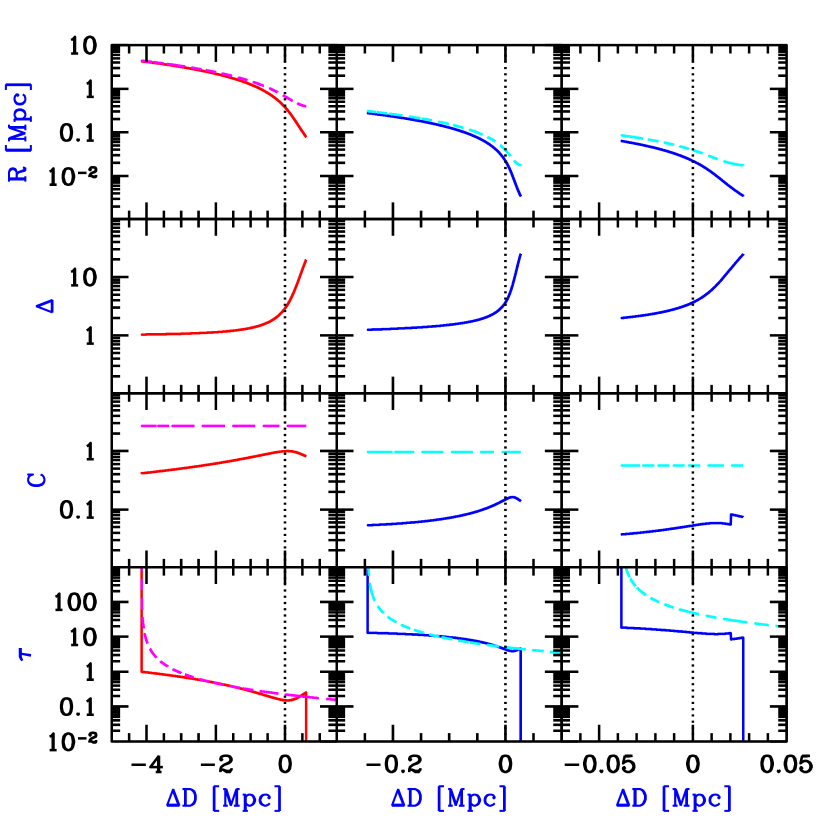
Figure 1.— Properties of the gas in the H II region versus relative apparent position $\Delta D$. Panels correspond to a GRB host with a normal stellar IMF (right panels) or a Pop III IMF (middle panels), and to a quasar (left panels), all at redshift 7 in a region that had not been pre-ionized (note the different $\Delta D$ ranges; see text for the values of the input parameters). From bottom to top, panels show the Ly$\alpha$ optical depth due to resonant absorption ($\tau_{\rm res}$; solid curves) and due to the damping wing ($\tau_{\rm damp}$; dashed curves); the clumping factors $C_{{\rm Ly}\alpha}$ (solid curves) and $C_{x_{\rm H\,I}}$ (dashed curves); the gas overdensity due to infall; and the actual distance of each gas element from the ionizing source (solid curves), as well as the distance that the same gas element would have reached in the presence of pure Hubble expansion with no infall (dashed curves).

The figure shows the strong effect of infall, which produces resonant absorption well into the red wing (i.e., at $\Delta D>0$). In the case of pure Hubble flow, $\tau_{\rm res}$ would drop to zero right at $\Delta D=0$, and the drop would be gradual because of the increasing ionizing intensity at small distances from the source. When infall is included as part of a more realistic model, however, the infall velocity results in absorption of photons at $\Delta z>0$; furthermore, the value of $\tau_{\rm res}$ does not show a gradual drop since the high infall overdensity (and, therefore, high recombination rate) compensates for the high ionizing intensity felt by gas near the source. The sudden drop in $\tau_{\rm res}$ is due to the inclusion of an accretion shock, which fully ionizes the gas and cuts off absorption very close to the source. The inclusion of a clumping distribution, and the dominance of voids in allowing transmitted flux, leads to a strong reduction in $\tau_{\rm res}$ (i.e., $C_{{\rm Ly}\alpha}$ is significantly smaller than $C_{x_{\rm H\,I}}$). In the quasar and Pop III star cases, helium is fully ionized throughout the H II region, but in the normal IMF case, the GRB host galaxy produces only a small He III region; the optical depth jumps at this radius, due to the lower gas temperature in the He II region, and the transition can be seen at $\Delta D=0.02$ Mpc.

The effective clumping factor for transmission ($C_{{\rm Ly}\alpha}$) varies over the range 0.03–1. On the other hand, the clumping factor $C_{x_{\rm H\,I}}$ is always much larger, although its value ($\sim$0.5–3) is still significantly lower than the values $\gtrsim$ 10 that previous studies have used which did not account for the rarity of high clump densities along a given line of sight. Since it is defined in terms of a ratio of neutral fractions [see eq. (8)], $C_{x_{\rm H\,I}}$ is essentially independent of both $\Delta$ and the ionizing intensity, and is simply a function of $\Delta_{\rm max}$. For the cases shown in the figure, the proper radius of the H II region and the value of $\Delta_{\rm max}$ are respectively 0.063 Mpc and 1.8 (right panels), 0.28 Mpc and 3.7 (middle panels) and 4.3 Mpc and 31 (left panels). On the other hand, $C_{{\rm Ly}\alpha}$ is dominated by low values of $\Delta_{C}$, is nearly independent of $\Delta_{\rm max}$, and is essentially a function of the no-clumping ($C=1$) optical depth, which itself is proportional to $\Delta^{2}R^{2}$, where we used the fact that the source ionizing intensity (which affects the neutral hydrogen fraction) is inversely proportional to $R^{2}$. Indeed, when the $C=1$ optical depth is large, the transmission in the voids (where $\tau_{\rm res}\propto\Delta_{C}^{2}$ is low) becomes increasingly dominant in the calculation of the overall mean transmission. Note that our results differ quanitatively from the clumping model of Haiman (2002), who found an effective clumping factor for transmission of $\sim 0.04$ when $\tau_{\rm res}=1$, while we obtain $C_{{\rm Ly}\alpha}\sim 0.4$ in this case.

The figure also shows that $\Delta\sim 20$ at the shock radius, although the infall pattern depends on the halo mass and redshift; at a given redshift, higher-mass halos correspond to rarer density peaks, which tends to strengthen the infall pattern around them, but in standard models there is less power on large scales and this works in the opposite direction [see Barkana (2004)]. Gas with large $\Delta$ is located at a real radius $R$ that is much smaller than the radius the same gas element would have reached in the absence of infall; this is consistent with mass conservation. Observations of $\tau_{\rm res}$ can in principle probe the density profile of cosmological gas infall all the way from the shock radius out to the radius of the H II region, a range that represents $\sim 1.5$ orders of magnitude of $R$. Note that for each gas element, the total velocity relative to $z_{S}$ is $H(z_{S})\,\Delta D$, while the Hubble velocity component is $H(z_{S})\,R$, where the Hubble constant at high redshift is accurately approximated by

$$H(z)=835\,\left(\frac{1+z}{8}\right)^{3/2}\,\left(\frac{\Omega_{m}h^{2}}{0.136}\right)^{1/2}\,{\rm\ km\ s^{-1}\ Mpc^{-1}}\ .$$ (18)

The main conclusion from this figure is that a quasar affects a much larger surrounding region than a typical GRB host, both in terms of infall and ionization. Specifically, the region of significant infall (measured by $\Delta>2$) is larger by a factor of $\sim 10$ in radius, or 1000 in volume. Likewise, the H II region radius is larger by a factor $>10$ even compared to a GRB host with an extreme Pop III population of stars. Furthermore, within the H II region itself, $\tau_{\rm res}$ is of order unity for a quasar, and of order 10 in the GRB case. This means that absorption in this region can be easily probed in quasars, while for GRB hosts the absorption is near total except well into the damping wing; note that at larger $\Delta D$, beyond the limits shown in the figure, $\tau_{\rm damp}$ continues to decrease roughly inversely with $\Delta D-\Delta D_{\rm II}$, where $\Delta D_{\rm II}<0$ is the apparent position of the edge of the H II region. Thus, cosmological infall is pronounced around quasars and its effects are observable over a large region, while it is weak in GRB hosts and essentially unobservable. On the other hand, the damping wing can be observed in GRB hosts over a large region to the red side of resonant absorption, while in quasars $\tau_{\rm damp}\ll 1$ except in the region where $\tau_{\rm res}$ is of comparable importance.

Note that we have not solved for exact radiative transfer in the expanding H II region, but instead have assumed that the region is optically thin when we determined the ionizing intensity at various positions within the region. In order to check this assumption, we calculate the optical depth $\tau_{\rm ion}$ to hydrogen-ionizing photons from the source being absorbed as they travel out to the edge of the H II region. This optical depth depends on the intensity and gas density at all radii through the region. In order to place an upper limit on the optical depth, we evaluate it for photons with an energy just above the ionization threshold of hydrogen. For the three cases shown in the figure, $\tau_{\rm ion}$ thus defined equals 0.019 (normal GRB host), 0.027 (Pop III GRB host) and 0.015 (quasar). The fact that $\tau_{\rm ion}\ll 1$ justifies the neglect of radiative absorption and scattering in our calculations.

4. Detecting Cosmological Infall around Quasars

As illustrated in the previous section, observations of Ly$\alpha$ absorption in quasars can probe the cosmological infall pattern induced by the dark matter halo surrounding each quasar. In this section, we predict the dependence of the absorption pattern on the quasar redshift and flux. If these trends predicted by theory can be checked directly in observations, then this would test the fundamental properties of quasars and of dark matter halos, as well as the correlation between them.

Quasars have broad-band spectra that, due to their high luminosity, can be measured accurately even at high redshift. However, unlike GRB afterglows, the spectra are composed of emission lines broadened by multiple components of moving gas, and the difficulty in predicting the precise shape of, e.g., the Ly$\alpha$ line in any particular quasar presents a significant systematic error in determinations of the absorption profile. A promising approach is to adopt the parametrized form of the emission profile that best fits the line shape of most quasars at low redshift, and then fix the parameters for each quasar based on the part of the Ly$\alpha$ line that does not suffer resonant absorption (Barkana & Loeb, 2003). Quasars also have important advantages. The great intensity of quasars highly ionizes their host galaxies and reduces the amounts of gas and dust, thus simplifying the analysis. Furthermore, if the relatively high metallicity found for high-redshift quasars is typical of quasars at even higher redshifts, then various metal lines may be detected in addition to Ly$\alpha$, allowing an independent measure of the host redshift and of the velocity structure of the gas producing the broad emission lines.

We can easily understand the rough scaling with the observable parameters (i.e., quasar luminosity and redshift) of the properties of the red absorption drop due to infall. The luminosity of a quasar at redshift $z_{S}$ is proportional to $M_{\rm BH}$ times $f_{E}$, the fraction of the Eddington luminosity that is actually emitted by a given quasar. We assume here a general power-law relation $M_{\rm BH}\propto V_{c}^{n}$ between the black hole mass and the halo circular velocity (note that we adopt $n=5$ in the numerical results, as discussed in §2.3). The distance to the accretion shock is proportional to the halo virial radius, and the infall velocity of the pre-shock gas is proportional to the halo circular velocity. Thus, the wavelength offset of the absorption drop (measured redward from the central wavelength of the source Ly$\alpha$ emission) is

$$\Delta\lambda_{\rm drop}\propto(1+z_{S})\,\left(\frac{L}{f_{E}}\right)^{1/n}.$$ (19)

The halo mass is given by $M\propto(1+z_{S})^{-3/2}\,V_{c}^{3}$, or

$$M\propto(1+z_{S})^{-3/2}\,\left(\frac{L}{f_{E}}\right)^{3/n}\ .$$ (20)

The optical depth at the absorption drop is the Gunn-Peterson optical depth at that redshift, times the relative gas density $\Delta$, times the neutral hydrogen fraction. The neutral fraction is proportional to the gas density over the ionizing intensity, where the intensity is proportional to the quasar luminosity over the square of the distance to the accretion radius. Thus, the optical depth scales as

$$\tau_{\rm drop}\propto\Delta^{2}(1+z_{S})^{3/2}\,\frac{L^{(2-n)/n}}{f_{E}^{\,2/n}}\ ,$$ (21)

where $\Delta$ depends on $M$ and $z$ through the infall model. Note that the dependence of optical depth directly on halo mass is

$$\tau_{\rm drop}\propto\Delta^{2}(1+z_{S})^{(5-n)/2}f_{E}^{\,-1}M^{(2-n)/3}\ .$$ (22)

Also note that clumping (§ 2.2) modifies slightly these scalings of the optical depth. Observing the absorption drops in quasars over a wide range of luminosity and redshift will probe the population of quasars and the properties of their halos through the values of $f_{E}$, $\Delta$, and $n$.

Figure 2 shows the fraction of the quasar’s flux that is transmitted through the surrounding, infalling IGM. We assume a quasar at redshift 6 that had turned on after reionization, and we therefore include only resonant absorption. We consider a quasar with a flux typical of the recent SDSS high-redshift quasars, and also compare to quasars with fluxes lower by a factor of 10 or 100, applicable to future surveys. In each case, we translate the flux to black hole mass by assuming that the quasar radiates at the Eddington luminosity. We also compare to the case where the quasar is instead assumed to be radiating at only $10\%$ of Eddington; in this case the black hole must be more massive in order to produce a given observed flux, implying a larger surrounding halo, and an absorption drop more strongly shifted to the red (corresponding to a larger infall velocity). As implied by the scalings presented above, fainter quasars at a given redshift have a smaller incursion of absorption into the red wing of Ly$\alpha$; they also have a larger $\tau_{\rm drop}$ since the slightly smaller $\Delta$ around lower-mass hosts does not compensate for the lower luminosity of the quasars.

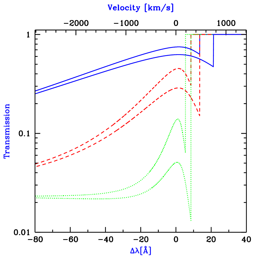
Figure 2.— Transmission fraction of a quasar’s flux through the infalling intergalactic medium, as a function of wavelength (or velocity) relative to the center of the quasar’s emission line. The quasar is assumed to have an observed flux $F_{\lambda}$ of 1 (solid curves), 0.1 (dashed curves), or 0.01 (dotted curves), in units of $10^{-17}$ erg cm^-2 s^-1 Å ^-1. In each pair of curves, the quasar is assumed to be radiating at its Eddington luminosity (top) or at $10\%$ of Eddington (bottom). All curves are at redshift 6 and assume that the quasar had turned on after reionization.

The transmitted flux fraction is also shown in Figure 3, but for various quasar redshifts. For a given observed flux, lower-redshift quasars are situated inside smaller hosts, and the absorption profiles are seen to have a smaller $\Delta\lambda_{\rm drop}$ along with a slightly lower $\tau_{\rm drop}$. For $z_{S}=7$, a quasar emitting inside a still neutral region is distinguished by the appearance of the damping wing. In addition, such a quasar has a significantly smaller red absorption drop because of the higher temperature of gas reionized by the relatively hard quasar spectrum; the recombination rate is lower in such gas, thus reducing the hydrogen neutral fraction and the Ly$\alpha$ optical depth.

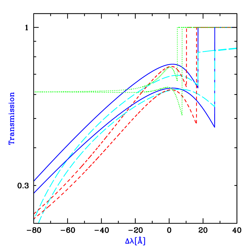
Figure 3.— Transmission fraction of a quasar’s flux through the infalling intergalactic medium, as a function of wavelength relative to the center of the quasar’s emission line. The quasar is assumed to have an observed flux $F_{\lambda}$ of $10^{-17}$ erg cm^-2 s^-1 Å ^-1, and to be in a post-reionization universe at redshift 7 (solid curves), 5 (short-dashed curves), or 3 (dotted curves). Also shown is the same redshift 7 quasar but assuming that it reionized its surroundings for the first time over a time $t_{S}=2\times 10^{7}$ yr (long-dashed curves). In each pair of curves, the quasar is assumed to be radiating at its Eddington luminosity (top) or at $10\%$ of Eddington (bottom).

In both figures, apparent at large distances from the quasar is the contribution of the mean ionizing background, which is included at redshift 6 and below but is most prominent at redshift 3. In addition, the appearance of the red-most absorption feature, and the shape of the rise and then the fall of the transmission toward shorter wavelengths, vary widely depending on the properties of the quasar, its halo, and the surrounding infall region. In principle, the precise shape of the absorption profile can be used to measure the detailed gas density profile in addition to the basic parameters of the quasar and its host halo. However, these transmission profiles cannot be directly observed; for any particular quasar, the transmission profile operates on the intrinsic profile of the quasar emission, and density fluctuations along the line of sight change the transmission relative to the ensemble-averaged profile. While these complications can be modeled, we have focused here on the observable features that are independent of these uncertainties and that are recognizable even in individual spectra, although the precise values may fluctuate compared to the ensemble-averaged ones; specifically, these features are the magnitude of the red absorption drop, and its location in wavelength, which is most useful if the quasar redshift is measured accurately, e.g., from other emission lines. For a statistical sample of quasars, our results should best match the ensemble-averaged spectrum.

5. Probing Reionization with $\gamma$-ray Burst Afterglows

Gamma-Ray Burst (GRB) explosions from the first generation of stars offer a particularly promising opportunity to probe the epoch of reionization. Young (days to weeks old) GRBs are known to outshine their host galaxies in the optical regime at $z\sim 1-3$. In hierarchical galaxy formation in $\Lambda$CDM, the characteristic mass and hence optical luminosity of galaxies and quasars declines with increasing redshift; hence, GRBs should become easier to observe than galaxies or quasars at increasing redshift. If the first stars are preferentially massive (Abel, Bryan, & Norman, 2002; Bromm, Coppi, & Larson, 2002) and GRBs originate during the formation of compact stellar remnants such as neutron stars and black holes, then the fraction of all stars that end up as GRB progenitors may be even higher at early cosmic times.

Similarly to quasars, GRB afterglows possess broad-band spectra which extend into the rest-frame UV and can probe the ionization state and metallicity of the IGM out to the epoch when it was reionized (Lamb & Reichart, 2000). Simple scaling of the long-wavelength spectra and temporal evolution of afterglows with redshift implies that at a fixed time lag after the GRB trigger in the observer’s frame, there is only a mild change in the observed  flux at infrared or radio wavelengths as the GRB redshift increases (Ciardi & Loeb, 2000). Hence, GRBs provide exceptional lighthouses for probing the universe at high redshift. The infrared spectrum of GRB afterglows occurring around the reionization redshift could be taken with future telescopes such as the James Webb Space Telescope (JWST; see http://www.jwst.nasa.gov/), as a follow-up on their early X-ray localization with the Swift  satellite. In this section, we explore how such a spectrum could reveal the damping wing due to neutral IGM, and thus probe reionization.

If GRBs originate from stellar remnants of high-mass stars, then they are expected to occur in host galaxies with a probability proportional to the SFR of each galaxy. In order to specify a typical host, we estimate as follows the SFR of galaxies in halos of various mass $M$ at redshift $z=7$. We assume that the SFR in a given halo is proportional to $M$ divided by a star-formation timescale which is determined by the halo merger history. Specifically, we estimate the age of gas in a given halo using the average rate of mergers which built up the halo. Based on the extended Press-Schechter formalism (Lacey & Cole, 1993), for a halo of mass $M$ at redshift $z$, the fraction of the halo mass which by some higher redshift $z_{2}$ had already accumulated in halos with galaxies is

$$F_{M}(z,z_{2})={\rm erfc}\left(\frac{1.69/D(z_{2})-1.69/D(z)}{\sqrt{2(S(M_{\rm min}(z_{2}))-S(M))}}\right)\ ,$$ (23)

where $D(z)$ is the linear growth factor at redshift $z$, $S(M)$ is the variance on mass scale $M$ (defined using the linearly-extrapolated power spectrum at $z=0$), and $M_{\rm min}(z_{2})$ is the minimum halo mass for hosting a galaxy at $z_{2}$. We assume that prior to the final phase of reionization this minimum mass is determined by the minimum virial temperature of $\sim 10^{4}$ K required for efficient atomic cooling in gas of primordial composition. We estimate the typical age of gas in the halo as the time since redshift $z_{2}$ where $F_{M}(z,z_{2})=0.5$, so that $50\%$ of the gas in the halo has fallen into galaxies only since then. The result at $z=7$ is that $M_{\rm min}(z=7)=1.3\times 10^{8}M_{\odot}$, $50\%$ of the total SFR occurs in halos up to $M=4\times 10^{8}M_{\odot}$, and $90\%$ in halos up to $M=5\times 10^{9}M_{\odot}$.

The GRB afterglow spectrum can be modeled as a set of power-law segments. Regardless of the particular power law which applies to the Ly$\alpha$ region, since the wavelength band relevant for H I absorption is narrow, the intrinsic afterglow emission is essentially constant over this region; e.g., at $z=7$, the flux level should vary by $\lesssim 1\%$ over a range of $\Delta\lambda=100$Å around the redshifted Ly$\alpha$ wavelength. Thus, the GRB afterglow offers a unique opportunity to detect the signature of IGM absorption, if the afterglow spectrum is at all similar to the theoretically expected smooth spectrum. The following numerical expressions and figures are based on the model of Sari, Piran, and Narayan (1998), corrected for a jet geometry using Sari, Piran, and Halpern (1999) [see also Waxman & Gruzinov (1999)].

Based on modeling of observed afterglows, we assume typical afterglow parameters of $E=10^{51}$ erg for the total (not isotropic) energy (Frail et al., 2001), a jet opening angle of $\theta=0.07$ rad, an external shock occurring in a surrounding medium of uniform density $n=1$ cm^-3, electrons accelerated to a power-law distribution of Lorentz factors with index $p=2.4$, and a fraction $\epsilon_{B}=10\%$ of the shock energy going to the magnetic field and $\epsilon_{e}=10\%$ to the accelerated electrons. We assume adiabatic evolution, and neglect synchrotron self-absorption which is only important at much lower frequencies than we consider.

Figure 4 shows quantitatively the detectability of GRB afterglows at redshifts $z=5$–15. The figure indicates that the redshifted Ly$\alpha$ region of GRB afterglows remains sufficiently bright for a high-resolution study with JWST  up to several weeks after the GRB explosion, throughout the redshift range we consider. Each light-curve of afterglow flux shows a couple of breaks over the range of times considered in the figure. We let $\nu_{m}$ and $\nu_{c}$ be the characteristic synchrotron frequencies (redshifted to the observer) of, respectively, the lowest-energy electron in the accelerated power-law distribution, and the lowest-energy electron that radiates efficiently enough to lose most of its energy. At early times the afterglow is in the fast cooling regime ($\nu_{m}>\nu_{c}$), when all the accelerated electrons cool efficiently, and the observed frequency $\nu_{\alpha}$ (corresponding to redshifted Ly$\alpha$) is intermediate between the two characteristic frequencies, leading to a spectral shape $F_{\nu}\propto\nu^{-0.5}$ near Ly$\alpha$. The first break occurs when $\nu_{\alpha}$ rises above $\nu_{m}$ at

$$t_{\rm obs} =6.8\,\left(\frac{E}{10^{51}\,{\rm erg}}\right)^{1/3}\,\left(\frac{\theta}{0.07\,{\rm rad}}\right)^{-2/3}\,\left(\frac{\epsilon_{B}}{0.1}\right)^{1/3}$$ (24)

$$\times\left(\frac{\epsilon_{e}}{0.1}\right)^{4/3}\,\left(\frac{1+z_{S}}{8}\right)\,{\rm hrs}\ .$$

After this break, $\nu_{\alpha}$ is bigger than both $\nu_{m}$ and $\nu_{c}$, and $F_{\nu}\propto\nu^{-p/2}$ near Ly$\alpha$. The second break, which is due to sideways expansion of the jet, affects the light-curve but not the spectral slope near Ly$\alpha$. It occurs at

$$t_{\rm obs} =3.5\,\left(\frac{E}{10^{51}\,{\rm erg}}\right)^{1/3}\,\left(\frac{\theta}{0.07\,{\rm rad}}\right)^{2}$$ (25)

$$\times\left(\frac{n}{1\,{\rm cm}^{-3}}\right)^{-1/3}\,\left(\frac{1+z_{S}}{8}\right)\,{\rm days}\ .$$

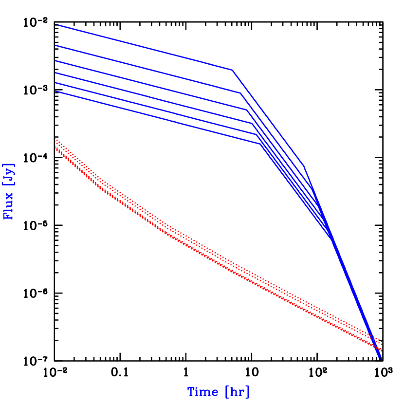
Figure 4.— Detectability of high-redshift GRB afterglows as a function of time since the GRB explosion as measured by the observer. The GRB afterglow flux is shown (solid curves) at the redshifted Ly$\alpha$ wavelength. Also shown (dotted curves) is the detection threshold for JWST  assuming a spectral resolution $R=5000$ with the near infrared spectrometer, a signal to noise ratio of 5 per spectral resolution element, and an exposure time equal to $20\%$ of the time since the GRB explosion. In each set of curves, a sequence of redshifts is used, $z=5$, 7, 9, 11, 13, and 15, respectively, from top to bottom.

As noted earlier, afterglows fade only slowly with redshift, since a given observed time corresponds to an earlier source time for high redshift afterglows, which are thus intrinsically brighter. Indeed, after the second break, the Ly$\alpha$ flux at a given $t_{\rm obs}$ is enhanced by this effect in proportion to $(1+z_{S})$ to the power $p$, a factor that for $p=2.4$ almost overcomes the fading according to the inverse squared luminosity distance. GRB afterglows may be even more easily detectable than indicated in figure 4 if a significant fraction exhibit an early UV-optical flash from a reverse external shock; e.g., the flash in GRB 990123 at $z=1.6$ was detected at a flux level of $\sim 1$ Jy at rest-frame $\lambda\sim 2000$Å about 50 seconds after the burst began (Akerlof et al., 1999).

Relative to other possible sources, GRB afterglows offer the advantage of having smooth, power-law spectra, which helps GRBs avoid the systematic uncertainties associated with the need to model the Ly$\alpha$ emission profiles of galaxies and quasars. In addition, GRBs are expected to occur mainly in relatively low mass halos, which induce only weak infall of the surrounding gas and produce insignificant H II regions, as illustrated in § 3. Metal lines from the host may be seen in absorption in the afterglow spectrum, thus allowing an accurate redshift measurement. Emission from the host galaxy should not significantly contaminate the early afterglow, but it may make the galaxy marginally detectable with JWST  once the afterglow has faded away. For instance, $10\%$ of the SFR at $z=7$ occurs in halos above $M=5\times 10^{9}M_{\odot}$, and a halo of this mass is expected to have a SFR of $\sim 1M_{\odot}$ per year, which translates [for a normal IMF] to a 1500Å continuum flux density of $\sim 15$ nJy, and a flux density in the $\sim 10$Å bandwidth of the Ly$\alpha$ line emission from the galaxy of $\sim 500$ nJy. If the star-forming regions where GRBs are expected to occur contain significant column densities of gas and dust, then they may contaminate the signal from IGM absorption, as discussed in § 2.6.

Figure 5 illustrates GRB afterglow absorption profiles (top panel) and explores the possibility of contamination from dust and neutral gas in the host (bottom panel). If absorption from the host is negligible then GRB afterglows offer a clear and direct measurement of absorption by the damping wing of H I in the IGM. In particular, the sharp cutoff expected if only resonant absorption is included (bottom panel, dot-long dashed curve) is easily distinguishable from the gradual cutoff characteristic of absorption by the damping wing (bottom panel, solid curve). In this case, the IMF can be constrained as well, since a strongly-ionizing IMF produces a gradual cutoff as well as a sharp drop due to resonant absorption (top panel, dashed curves); this occurs since the neutral gas lies further away (in the blue wing), producing a relatively weak damping wing that is interrupted by the ubiquitous red-wing drop due to resonant absorption.

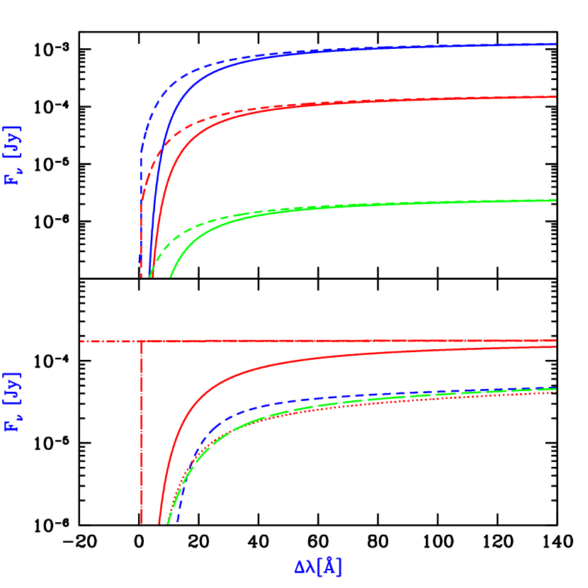
Figure 5.— IGM absorption profiles in GRB afterglows, presented in terms of the flux density $F_{\nu}$ versus relative observed wavelength $\Delta\lambda$. All curves adopt $z=7$ (assumed prior to the final reionization phase) and the typical halo mass $M=4\times 10^{8}M_{\odot}$ expected for GRB host halos. Top panel: Predicted spectrum including IGM H I absorption (both resonant and damping wing), for host galaxies with $t_{S}=10^{7}$ yr, $f_{\rm esc}=10\%$ and a normal IMF (solid curves) or $t_{S}=10^{8}$ yr, $f_{\rm esc}=90\%$ and a Pop III IMF (dashed curves). The observed time after the burst is one hour, one day, and ten days, from top to bottom, respectively. Bottom panel: Predicted spectra one day after a GRB for a host galaxy with $t_{S}=10^{7}$ yr, $f_{\rm esc}=10\%$ and a normal IMF. Shown is the unabsorbed GRB afterglow (dot-short dashed curve, essentially horizontal), the afterglow with resonant IGM absorption only (dot-long dashed curve), and the afterglow with full (resonant and damping wing) IGM absorption (solid curve). Also shown, with 1.7 magnitudes of extinction, are the afterglow with full IGM absorption (dotted curve), and attempts to fit this profile with a damped Ly$\alpha$ absorption system in the host galaxy (dashed curves; see text).

However, as illustrated in the bottom panel of figure 5, contamination by absorption in the host galaxy may hamper studies of reionization and of the IMF based on absorption profiles. The three lower curves include extinction as might be produced by an H I column density of $10^{21}\,{\rm cm}^{-2}$ [see eq. (16)]. Because of its relatively smooth spectrum, extinction does not significantly change the shape of the absorption profile; moreover, it is possible to take advantage of the broad-band afterglow spectrum in order to derive the effect of extinction near redshifted Ly$\alpha$ by measuring the extinction over a much wider range of wavelengths than shown in the figure and interpolating into the critical bandpass. However, extinction does lower the overall flux and thus increases the integration time required to measure an accurate spectrum.

As shown in figure 4, at $t_{\rm obs}=1$ day, a minimum flux of $F_{\nu}\sim 10^{-6}$ Jy is needed for a high-resolution spectrum with JWST.  Assuming a spectrum obtained with this sensitivity, we consider whether absorption by a large H I column density in the host could be confused with the signature of the IGM damping wing before reionization. We consider only the $F_{\nu}>10^{-6}$ Jy portion of the profile with extinction and full absorption due to the IGM (figure 5, bottom panel, dotted curve), and attempt to reproduce this profile by replacing the IGM damping wing with a damped Ly$\alpha$ system in the galactic host. If the host redshift is precisely known, the different shapes of the two gradual cutoffs preclude any possibility of confusion between them. For example, a damped Ly$\alpha$ system with $N_{\rm H\,I}=2\times 10^{20}\,{\rm cm}^{-2}$ (short-dashed curve) is 1.5 orders of magnitude too low at $\Delta\lambda\sim 10$Å and 10–20$\%$ too high at $\Delta\lambda=30$–100Å.

However, if the source redshift is not measured exactly then a much closer match is possible. The damped Ly$\alpha$ system (long-dashed curve) that most closely simulates the effect of the IGM damping wing in this case has $N_{\rm H\,I}=7.7\times 10^{20}\,{\rm cm}^{-2}$ and is shifted blueward by $\Delta\lambda=-15.4$Å, equivalent to $\Delta z$ = 0.013 or a velocity blueshift of 500 km s^-1. This match, although it appears fairly close in the figure, is off at various wavelengths by a difference ranging between $-6\%$ and $+6\%$, and this difference should be easily measurable. However, the relatively close match in this comparison of a pure IGM damping wing with a pure damped Ly$\alpha$ system suggest that in a realistic situation, when both may contribute, this partial degeneracy will limit the constraints that can be derived on the various parameters of interest. Note, though, that since the halo circular velocity is only $\sim 24$ km s^-1, the peculiar velocity of the GRB (which may arise from the circular velocity of the disk) is negligible, and an accurate redshift measurement can help to break the near-degeneracy. Regarding another possible difficulty, Miralda-Escudé (1998) showed that $\sim 10\%$ uncertainties in the cosmological parameters would contribute further to the near-degeneracy between a damped Ly$\alpha$ system and the IGM damping wing, but this factor continually becomes less important as various cosmological probes yield increasingly precise parameter values (e.g., Spergel et al., 2003).

The hydrogen absorption within the host galaxy of the GRB should be reduced by the early ionizing radiation of the GRB afterglow itself (Perna & Loeb, 1998). The recombination time of the surrounding interstellar medium ($\sim 10^{5}n_{0}^{-1}~{}{\rm yr}$) is long compared to the duration of the afterglow emission, where $n_{0}$ is the medium density in units of ${\rm cm^{-3}}$. Hence, each ionizing photon will eliminate a neutral hydrogen atom from the interstellar medium along the line of sight. Given that the number of hydrogen atoms out to a distance $r$ is $\propto n_{0}r^{3}$, the radius ionized by a given afterglow varies as $n_{0}^{-1/3}$. Draine & Hao (2002) showed that an early optical/UV flash should ionize hydrogen and destroy dust and molecular hydrogen out to a distance of $\sim 10^{19}$ cm in surroundings of $n_{0}\sim 10^{3}-10^{4}$ (see also Perna & Loeb, 1998; Waxman & Draine, 2000; Draine, 2000; Fruchter, Krolik, & Rhoads, 2001; Perna & Lazzati, 2002; Perna, Lazzati, & Fiore, 2003). Therefore, the early afterglow emission could significantly reduce the damped Ly$\alpha$ absorption within a host molecular cloud ($n_{0}\sim 10^{4}$, $r\sim 10$ pc) or a line of sight passing at an angle through a host galactic disk ($n_{0}\sim 1$, $r\sim 100$ pc). However, the afterglow’s characteristic sphere of influence is negligible compared to the intergalactic scales of interest for reionizing the IGM.

6. Conclusions

We have calculated the profile of Ly$\alpha$ absorption for GRBs and quasars during and after the epoch of reionization, including the effects of ionization by the source and its host galaxy, clumping, and cosmological infall of the surrounding cosmic gas. We find that GRBs are the optimal probes of the ionization state of the surrounding IGM as they are most likely to reside in dwarf galaxies that do not significantly perturb their cosmic environment. On the other hand, bright quasars reside in the most massive galaxies and probe the strong gravitational effects of these galaxies and their halos on the IGM.

In order to isolate the intergalactic contribution to the Ly$\alpha$ damping wing, it is necessary to measure the source redshift accurately. Here again, GRB afterglows are simpler to interpret. In quasars, although there are often strong emission lines in addition to Ly$\alpha$, bulk motions can shift them substantially from the systemic redshift of the host galaxy. For example, some broad emission lines such as C IV are typically offset by $\sim 1000$ km s^-1, but low-ionization broad lines such as Mg II are only offset by $\sim 200$ km s^-1 (Richards et al., 2002). The Mg II line can be detected at high redshift in the near-infrared and, indeed, it has been observed for the highest redshift quasar known (Willott, McLure, & Jarvis, 2003). Redshifts accurate to better than 100 km s^-1 may be obtainable by detecting narrow lines such as [O III], perhaps marginally possible from the ground or else doable with JWST.  For either a GRB or a quasar, however, perhaps the best method for determining its redshift is to detect molecular emission or absorption lines in the interstellar medium of its host galaxy. The resulting measurement is likely to be accurate to within the disk velocity dispersion, which should be rather low, particularly in the low-mass hosts that are typical of GRBs. These lines can be detected at high redshift, as demonstrated by the CO emission from the host galaxy of the highest-redshift quasar known (Fabian et al., 2003). Note that another possible disadvantage of quasars is that their massive hosts may develop significant peculiar velocities as they are likely to reside in rare high-density environments such as groups of galaxies.

Supernova and quasar outflows could change our predictions if they reached out from the galaxy far enough to affect the gas at the distances where it produces the absorption in our model. Although outflowing gas can be detected spectrally and the outflow velocity deduced, it is generally very difficult to determine the spatial scale of an outflow around a high-redshift galaxy. Adelberger et al. (2003) have detected a statistical signature based on six objects that suggests that Lyman break galaxies at $z\sim 3$–4 produce outflows that drive away surrounding gas out to a radius of $\sim 0.5\ h^{-1}$ comoving Mpc. If this preliminary signal is correct, and if these Lyman break galaxies lie in $M\gtrsim 10^{12}M_{\odot}$ host halos, then these outflows reach a distance comparable to the halo accretion shock and may begin to marginally affect our model predictions. Note that direct absorption by the outflowing gas should generally be distinguishable from the absorption patterns that we predict. Absorption from outflows should occur in the blue wing and thus not interfere with the red absorption feature due to infall. Furthermore, outflowing gas is likely to be highly enriched and can be probed (or ruled out) in each object using metal lines.

High-redshift GRB afterglows are likely to open a new frontier in extragalactic astronomy (“GRB cosmology”), by providing important new clues about their progenitors — the first stars — and about the reionization history of the intervening IGM. Afterglow spectra can also be used to explore the metal enrichment history of the IGM through the detection of intergalactic metal absorption lines (Furlanetto & Loeb, 2003). The comparison between observed spectra of high-redshift afterglows and detailed cosmological simulations of the IGM (involving hydrodynamics and radiative transfer during the epoch of reionization) will provide a better understanding of the process of galaxy formation in the young universe, only $\sim 10^{8}$–$10^{9}$ years after the big bang.

References

- Abel, Bryan, & Norman (2002) Abel, T., Bryan, G. L., & Norman, M. L. 2002, Science, 295, 93
- Abel & Haehnelt (1999) Abel, T., & Haehnelt, M. G. 1999, ApJ, 520, L13
- Adelberger et al. (2003) Adelberger, K. L., Steidel, C. C., Shapley, A. E., & Pettini, M. 2003, ApJ, 584, 45
- Akerlof et al. (1999) Akerlof, C. W., Balsano, R., Barthelmy, S. et al. 1999, Nature, 398, 400
- Bajtlik, Duncan, & Ostriker (1988) Bajtlik, S., Duncan, R. C., & Ostriker, J. P. 1988, ApJ, 327, 570
- Barkana (2002) Barkana, R. 2002, New Astronomy, 7, 85
- Barkana (2004) Barkana, R. 2004, MNRAS, in press (preprint astro-ph/0212458)
- Barkana & Loeb (2001) Barkana, R. & Loeb, A. 2001, Phys. Rep., 349, 125
- Barkana & Loeb (2002) Barkana, R., & Loeb, A. 2002, ApJ, 578, 1
- Barkana & Loeb (2003) Barkana, R. & Loeb, A. 2003, Nature, 421, 341
- Becker et al. (2001) Becker, R. H., Fan, X., White, R. L., et al. 2001, AJ, 122, 2850
- Bernardi et al. (2003) Bernardi, M., et al. 2003, AJ, 125, 32
- Blain & Natarajan (2000) Blain, A. W., & Natarajan, P. 2000, MNRAS, 312, L35
- Bloom et al. (2002) Bloom, J. S., Kulkarni, S. R., & Djorgovski, S. G. 2002, AJ, 123, 1111
- Bohlin, Savage, & Drake (1978) Bohlin, R. C., Savage, B. D., & Drake, J. F. 1978, ApJ, 224, 132
- Bond et al. (1991) Bond, J. R., Cole, S., Efstathiou, G., & Kaiser, N. 1991, ApJ, 379, 440
- Bromm, Coppi, & Larson (2002) Bromm, V., Coppi, P. S., & Larson, R. B. 2002, ApJ, 564, 23
- Bromm & Loeb (2002) Bromm, V., & Loeb, A. 2002, ApJ, 575, 111
- Bromm, Kudritzki, & Loeb (2001) Bromm, Kudritzki, & Loeb, 2001, ApJ, 552, 464
- Carilli, Gnedin, & Owen (2002) Carilli, C. L., Gnedin, N. Y., & Owen, F. 2002, ApJ, 577, 22
- Cen (2003) Cen, R. 2003, ApJ, 591, L5
- Cen & Haiman (2000) Cen, R., & Haiman, Z. 2000, ApJ, 542, L75
- Ciardi & Loeb (2000) Ciardi, B., & Loeb, A. 2000, ApJ, 540, 687
- Di Matteo, Perna, Abel, & Rees (2002) Di Matteo, T., Perna, R., Abel, T., & Rees, M. J. 2002, ApJ, 564, 576
- Draine (2000) Draine, B. T. 2000, ApJ, 532, 273
- Draine & Hao (2002) Draine, B. T. & Hao, L. 2002, ApJ, 569, 780
- Fabian et al. (2003) Fabian, W., et al. 2003, Nature, 424, 406
- Fan et al. (2002) Fan, X., Narayanan, V. K., Strauss, M. A., White, R. L., Becker, R. H., Pentericci, L., & Rix, H. 2002, AJ, 123, 1247
- Ferrarese & Merritt (2000) Ferrarese, L., & Merritt, D. 2000, ApJ, 539, L9
- Fitzpatrick (1999) Fitzpatrick, E. L. 1999, PASP, 111, 63
- Frail et al. (2001) Frail, D. A. et al. 2001, ApJ, 562, L55
- Fruchter, Krolik, & Rhoads (2001) Fruchter, A., Krolik, J. H., & Rhoads, J. E. 2001, ApJ, 563, 597
- Furlanetto & Loeb (2002) Furlanetto, S. R. & Loeb, A. 2002, ApJ, 579, 1
- Furlanetto & Loeb (2003) Furlanetto, S. R. & Loeb, A. 2003, ApJ, 588, 18
- Furlanetto, Sokasian, & Hernquist (2003) Furlanetto, S. R., Sokasian, A. & Hernquist, L. 2003, MNRAS, submitted (preprint astro-ph/0305065)
- Gunn-Peterson (1965) Gunn, J. E., & Peterson, B. A. 1965, ApJ, 142, 1633
- Haiman (2002) Haiman, Z. 2002, ApJ, 576, L1
- Haiman & Cen (2002) Haiman, Z., & Cen, R. 2002, ApJ, 578, 702
- Heger et al. (2003) Heger, A., Fryer, C. L., Woosley, S. E., Langer, N., & Hartmann, D. H. 2003, ApJ, 591, 288
- Iliev, Shapiro, Ferrara, & Martel (2002) Iliev, I. T., Shapiro, P. R., Ferrara, A., & Martel, H. 2002, ApJ, 572, L123
- Keshet et al. (2003) Keshet, U., Waxman, E., Loeb, A., Springel, V., & Hernquist, L. 2003, ApJ, 585, 128
- Kulkarni et al. (2000) Kulkarni, S. R. et al. 2000, Proc. SPIE, 4005, 9
- Lacey & Cole (1993) Lacey, C. G., & Cole, S. M. 1993, MNRAS, 262, 627
- Lamb & Reichart (2000) Lamb, D. Q., & Reichart, D. E. 2000, ApJ, 536, 1
- Leitherer et al. (1999) Leitherer, C., et al. 1999, ApJS, 123, 3
- Loeb (1996) Loeb, A. 1996, ApJ, 459, L5
- Loeb (2003) Loeb, A. 2003, in “Supernovae and Gamma-Ray Bursters”, ed. K. W. Weiler (Berlin: Springer), 445
- Loeb & Barkana (2001) Loeb, A. & Barkana, R. 2001, ARA&A, 39, 19
- Madau & Rees (2000) Madau, P., & Rees, M. J. 2000, ApJ, 542, L69
- Miralda-Escudé (1998) Miralda-Escudé, J. 1998, ApJ, 501, 15