Abstract

We investigate explosive nuclear burning in core collapse supernovae by coupling a tracer particle method to one and two-dimensional Eulerian hydrodynamic calculations. Adopting the most recent experimental and theoretical nuclear data, we compute the nucleosynthetic yields for 15 $M_{\odot}$ stars with solar metallicity, by post-processing the temperature and density history of advected tracer particles. We compare our results to 1D calculations published in the literature.

Chapter 0 Multi-dimensional nucleosynthesis calculations of Type II SNe

1 Introduction

The pre- and post-explosive nucleosynthesis of massive stars has been studied extensively by several groups over the last years (see Woosley & Weaver 1995; Thielemann et al. 1996; Limongi et al. 2000; Rauscher et al. 2002, and the references therein). Although a lot of work has been performed in this field, computed nucleosynthetic yields are still affected by numerous uncertainties. For instance, because of our rather sketchy current understanding of the physical mechanism(s) that lead from core collapse to supernovae (SNe), all studies of explosive nucleosynthesis, that have been performed to date, made use of ad hoc energy deposition schemes to trigger SN explosions in progenitor models. While the results of such calculations indicate that the yields of only a rather small number of nuclei are sensitive to the details of how the supernova shock is launched (see e.g. Woosley&Weaver 1995), it is nevertheless important to attempt to compute nucleosynthetic yields in the framework of more sophisticated models of the explosion. The impact of multidimensional hydrodynamics has not been investigated in detail so far. In addition, among the isotopes whose yields are known to depend sensitively on the explosion mechanism, and thus cannot be predicted accurately at present, are key nuclei, like $\rm{}^{56}Ni$ and $\rm{}^{44}Ti$, that are of crucial importance for the evolution of supernova remnants and for the chemical evolution of galaxies. These nuclei bare also important consequences for numerical supernova models. Their yields can be used as a sensitive probe for the conditions prevailing in SNe and hence can serve to constrain hydrodynamic SN models with their complex interdependence of neutrino-matter interactions and multi-dimensional hydrodynamic effects. This may ultimately aid in improving our understanding of the explosion mechanism itself.

2 Hydrodynamic models

The nucleosynthesis calculations presented in this work are based on one and two-dimensional hydrodynamic models of SNe which follow the revival of the stalling shock, which forms after iron core collapse, and its propagation through the star from 20 ms up to a few seconds after core bounce (when the explosion energy has saturated and all important nuclear reactions have frozen out). The simulations are started from post-collapse models of Rampp & Janka (priv. comm.), who followed core-collapse and bounce in the 15 $M_{\odot}$, $Z=Z_{\odot}$ progenitors of Woosley & Weaver (1995) and Limongi et al. (2000). We employ the HERAKLES code, which solves the hydrodynamic equations in 1, 2 or 3 spatial dimensions with the direct Eulerian version of the Piecewise Parabolic Method (Colella & Woodward 1984), and which incorporates the light-bulb neutrino treatment and the equation of state of Janka & Müller (1996) (for more details see Kifonidis et al. 2003, and the references therein). The main advantages of our approach are that we drive the shock by accounting for neutrino-matter interactions in the layers outside the newly born neutron star, instead of using a piston (see e.g. Woosley & Weaver 1995) or a “thermal bomb”, and the possibility to perform calculations from one up to three spatial dimensions. The main disadvantage is the fact that we do not take into account the dense innermost layers of the neutron star, and that we currently use a simplified scheme for neutrino transport. Thus, we cannot obtain self-consistent neutrino distribution functions, but have to assume the spectral distribution of neutrinos and anti-neutrinos of all flavors that are emitted by the neutron star, and the temporal evolution of their luminosities. We assume the latter to be given by the simple exponential law

$$L_{\nu_{i}}=L^{0}_{\nu_{i}}{\rm e}^{-t/t_{L}},(\nu_{i}\equiv\nu_{\rm e},\bar{\nu}_{\rm e},\nu_{\mu},\bar{\nu}_{\mu},\nu_{\tau},\bar{\nu}_{\tau})$$ (1)

where $t_{L}$ is of the order of $700$ ms, and the $L^{0}_{\nu_{i}}$ are parameters of the calculation. The neutrino spectra are prescribed in the same way as in Janka & Müller (1996).

3 Marker particle method

Choosing a hydrodynamic scheme for computing multi-dimensional hydrodynamic models that include the nucleosynthesis, one faces the dilemma of using either a Lagrangian or an Eulerian method. Since nuclear networks with hundreds of isotopes are prohibitively expensive in terms of CPU time and memory for multi-dimensional calculations, such networks can only be solved in a post-processing step (the energy source term due to nuclear burning can usually be calculated with a small network online with the hydrodynamics, and may even be neglected completely in some cases, depending on the structure of the progenitor). The Lagrangian approach has the advantage that it naturally yields the necessary data for the post-processing calculations, since it directly follows the evolution of specific fluid elements. For the problem of neutrino-driven supernovae, however, Lagrangian methods (like SPH) have a crucial drawback: by their nature they concentrate resolution in mass. Neutrino driven explosions, on the other hand, are triggered by neutrino heating in a high-entropy, low-density region outside the nascent neutron star. Failing to spatially resolve this region, which contains only a small amount of mass, will lead to arguable results regarding the hydrodynamics and thus ultimately to doubtful nucleosynthetic yields. To achieve an adequate spatial resolution, Eulerian schemes (where the grid is fixed in space) or even adaptive schemes (in which the grid automatically adapts to resolve steep gradients in the solution) are to be prefered. However, the problem then arises how one should obtain the necessary data for the post-processing calculations. We do this by adding a “Lagrangian component” to our Eulerian scheme in the form of marker particles that we passively advect with the flow in the course of the Eulerian calculation, recording their $T$ and $\rho$ history by interpolating the corresponding quantities from the underlying Eulerian grid. A similar method has been adopted in a previous study of multi-dimensional nucleosynthesis in core collapse SNe by Nagataki et al. (1997), and more recently in calculations for very massive stars (Maeda et al. 2002), and for Type Ia SNe (Niemeyer et. al. 2002).

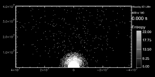
Figure 1: Initial marker particle distribution in the innermost 400 km of the computational domain of a 2D simulation that was started from the Woosley & Weaver (1995) progenitor. The entropy distribution (in $k_{b}$/nucleon) is depicted in the background.

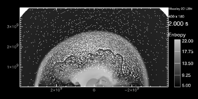
Figure 2: Final marker particle distribution of the 2D simulation from Fig. 1. Note the change of the radial scale, and the pile-up of particles in the dense layer between the (light colored) low-density, neutrino-heated bubble, which is almost void of markers, and the shock farther out. The entropy distribution (in $k_{b}$/nucleon) is depicted in the background.

For our 1D and 2D calculations we have used 1024 and 8000 marker particles, respectively. They are distributed homogeneously in mass throughout the progenitor’s Fe core, Si, O, and C shells assuming the composition of the progenitor at the corresponding mass coordinate as the initial composition of the respective tracer particle. Figure 1 shows the initial distribution of the particles in the innermost region of the computational domain for a 2D simulation that was started from the s15s7b progenitor of Woosley & Weaver (1995). The final distribution of the particles (at a time of 2 s after core bounce) is given in Fig. 2 for the same simulation. In both Figures the entropy distribution is plotted in the background. Figure 2 demonstrates that the particles trace mainly the high-density region of the ejecta (which is located between the shock and the neutrino-heated bubbles), and that still the spatial resolution of the hydrodynamic calculation is not compromised in the low-density, neutrino-heated layers due to the Eulerian nature of our hydrodynamic scheme.

4 Nucleosynthesis: first results and perspectives

Given the temperature and density history of individual marker particles we can calculate their nucleosynthetic evolution and compute the total yields (including the decays of unstable isotopes) as a sum over all particles. The reaction network employed for our nucleosynthesis calculations contains 296 nuclear species, from neutrons, protons, and $\alpha$-particles to $\rm{}^{78}Ge$ (F.-K. Thielemann, priv. comm.). The reaction rates include experimental and theoretical nuclear data as well as weak interaction rates. The ¹²C($\alpha$,$\gamma$)¹⁶O rate is that of Caughlan et al. (1985). To investigate the sensitivity of the yields with respect to the implementation of the nuclear physics, we have also recalculated the nucleosynthesis with the nuclear network code of M. Limongi (priv. comm.), and found good agreement with the results obtained using the Thielemann network code.

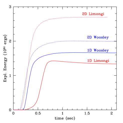
Figure 3: Explosion energies for diffferent models discussed in the text.

In order to estimate the effects of the spatial resolution of the hydrodynamic calculations on the nucleosynthetic yields we have performed resolution studies in one spatial dimension. Varying both the number of markers and Eulerian zones, we adjusted the numerical resolution such that errors resulting from interpolation between these two “grids” are less than a few per cent for a simulation with 2000 zones and 1024 marker particles. Keeping the resolution of the Eulerian grid fixed at 2000 zones and varying the number of markers, we obtain convergence of the yields, if the number of particles exceeds $\sim 1000$. For 10 times less markers, gradients in the hydrodynamic quantities are not sampled sufficiently accurately, affecting the final composition by $\sim$20%. Numerical convergence depends also on the accuracy of the hydrodynamic quantities themselves, i.e. on the resolution of the Eulerian grid. We have not investigated this in detail so far but plan to do this in forthcoming calculations. In addition, the one-dimensional results may not be applicable to the two-dimensional situation. Therefore, a resolution study in two spatial dimensions is also in preparation.

So far we have investigated four explosion models for their nucleosynthetic yields: a one-dimensional and a corresponding two-dimensional model that made use of model s15s7b of Woosley & Weaver (1995) and a second pair of a one and two-dimensional simulation for the 15 $M_{\odot}$ Limongi et al. (2000) progenitor. The properties of these models are given in Table 1, where $L^{0}_{\nu_{e},52}$ is the electron neutrino luminosity (in units of 10⁵² erg/s), $E_{exp,51}$ is the explosion energy (in units of 10⁵¹ erg), and $t_{exp}$ is the explosion time scale (in ms) defined as the time after the start of the simulation when the explosion energy exceeds 10⁴⁹ erg (for a detailed explanation of the neutrino parameters see Janka & Müller 1996 and Kifonidis et al. 2003).

Table 1: Parameters of models, using the Woosley&Weaver (1995, WW95) and Limongi et al. (2000, LSC00) progenitors.

Model	Zones	$N_{markers}$	$L^{0}_{\nu_{e},52}$	$E_{exp,51}$	$t_{exp}$ (ms)
1D WW95	2000	1024	2.940	1.46	230
2D WW95	400$\times$180	8000	2.940	1.99	125
1D LSC00	2000	1024	3.365	1.33	260
2D LSC00	400$\times$180	8000	3.365	2.69	150

Figure 3 shows the evolution of the explosion energy for the four models, using the same neutrino luminosity for the 1D and 2D model of the same progenitor. For both progenitors the 2D model explodes with higher energy than the corresponding 1D one. The Limongi et al. (2000) progenitor needs higher neutrino luminosity to explode, mainly due to the fact that it has a more compact core.

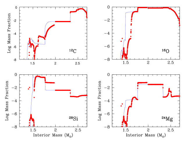
Figure 4: Logarithm of the final mass fractions (filled dots) of ¹²C,¹⁶O,²⁴Mg, and ²⁸Si as a function of mass coordinate for our 1D nucleosynthesis calculation employing the 15 $M_{\odot}$ Woosley & Weaver (1995) progenitor. Each dot represents a marker particle. The presupernova composition is also plotted (thin line).

In Fig. 4 we show the final mass fractions of ¹²C, ¹⁶O, ²⁴Mg, and ²⁸Si for the 1D calculation that made use of the Woosley & Weaver (1995) progenitor. Each dot represents a marker particle that is located at a certain mass coordinate and carries a specific composition. As a reference, we also plot the presupernova composition (Woosley & Weaver 1995). Comparing our 1D yields with the explosive nucleosynthesis results of Woosley & Weaver (1995), we find very good agreement (with small deviations of the order of few per cent) for the light elements. The position of the mass cut at 1.28 $M_{\odot}$ (which is obtained by comparing the velocity of each tracer particle with the local escape velocity) is in good agreement with the Woosley & Weaver (1995) result, too.

In Fig. 5 we compare the yields of the 1D and 2D simulation for the Woosley & Weaver (1995) progenitor. The differences, which are apparently negligible in case of the lighter nuclei and small for the heavier ones, are mainly due to the on average higher temperatures in the 2D simulation, i.e. more free neutrons are available in the innermost layers of the 2D simulation. This results in higher production factors for isotopes which are very sensitive to neutron captures, like e.g. ^46,48Ca, ^49,50Ti, ^50,51V, ⁵⁴Cr, and ⁶⁷Zn.

The reason for the rather small differences in the yields between the 1D and 2D simulation are the high initial neutrino luminosities, that we adopted for our calculations, and their rapid exponential decline. This leads to very rapid (and energetic) explosions (Fig. 3). The short explosion time scale prevents the convective bubbles, which form due to the negative entropy gradient in the neutrino-heated region, to merge to large-scale structures that can lead to global anisotropies, and hence to significant differences compared to the 1D case. Lowering the neutrino luminosities (and the explosion energies), we obtain stronger convection that strongly distorts the shock wave by developing large bubbles of neutrino-heated material (see Janka & Müller 1996; Kifonidis et al. 2000; Kifonidis et al. 2001; and Janka et al. 2001 for examples). Adopting constant core luminosities instead of the exponential law of Eq. (1), we can produce models where the phase of convective overturn lasts for several turn-over times and which exhibit the vigorous boiling behaviour reported by Burrows et al. (1995). Such cases can finally develop global anisotropies, showing a dominance of the $m=0$, $l=1$ mode of convection (see Janka et al. 2003; Scheck et al., in preparation). As a consequence, convection can lead to large deviations from spherical symmetry, and thus to larger differences in the final yields than those visible in Fig. 5. We are currently investigating such models in more detail.

Figure 5: Final mass fractions obtained for the 1D (dotted line) and 2D simulation (solid line) as a function of the atomic number, using the 15 $M_{\odot}$ Woosley & Weaver (1995) progenitor.

5 Electron captures in explosive conditions

A common result of nucleosynthesis studies that have been performed to date is that weak-interactions (in particular electron captures) do not play an important role for explosive nucleosynthesis conditions (i.e. for temperatures and densities obtained from artificially induced 1D explosions of Type II SN progenitors). In contrast, electron captures are known to be very important in presupernova hydrostatic nucleosynthesis (see e.g. the discussion in Woosley & Weaver 1995).

Figure 6: Mass fractions normalized to solar and to Fe abundance obtained for our 1D simulation using the Woosley & Weaver (1995) progenitor. The Woosley & Weaver yields are given by solid lines and filled dots. Our 1D simulation results including weak-interactions are shown by dot-dashed lines and crosses. Our 1D simulation results excluding weak-interactions are given by dotted lines and open squares.

In Fig. 6 we summarize the effect of electron captures on the yields of our 1D simulation that employs the Woosley & Weaver progenitor. The fact that markers with temperatures of $\sim 8\times 10^{9}$ K encounter high densities ($\geq 10^{8}$ g/cm³) leads to a large overproduction of neutron-rich Ni isotopes like ⁵⁸Ni and ⁶²Ni (from 100 up to 1000 times the solar value). According to our simulation (Fig. 7) markers with this composition are located at a mass coordinate $\sim$1.3 $M_{\odot}$ and have a typical Y_e of $\sim$0.48. As their velocity is higher than the local escape velocity, they have to be considered in the calculation of the final yields (unless there occurs late fallback, see below).

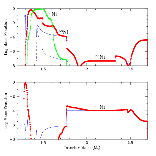
Figure 7: Logarithm of the mass fractions of ⁵⁶Ni and ⁵⁸Ni (upper panel) and ⁶²Ni (lower panel) as a function of mass coordinate for our 1D nucleosynthesis calculation employing the 15 $M_{\odot}$ Woosley & Weaver (1995) progenitor. Each dot (for ⁵⁸Ni and ⁶²Ni) and cross (for ⁵⁶Ni) represents a marker particle. The presupernova composition is also plotted (thin solid and dashed line).

Similar effects regarding the production of neutron-rich Ni isotopes as in the 1D case are found in the 2D model (see also the discussion regarding the differences between the 1D and 2D models in the previous Section). In addition, the 2D model causes a very high production of neutron-rich isotopes like ^46,48Ca, ^49,50Ti, ^50,51V, ⁵⁴Cr, and ⁶⁷Zn. Markers enriched in these isotopes are located in the innermost ejecta and have the lowest Y_e ($\sim$0.45). The fact that we obtain a high production of these isotopes only in the 2D model and not in 1D it is due to the higher temperatures reached in the innermost layers of the 2D simulation. This causes a higher degree of neutronization of these regions.

As we already mentioned it is possible that the overproduction problem might be resolved, at least in part, by late fallback. This, however, will most likely be only a viable solution for models with explosion energies that are significantly smaller than the ones that we have discussed here. Whether or not the overproduction problem can be solved will in addition depend on the efficiency of Rayleigh-Taylor mixing during the late-time evolution. Several episodes of deceleration (accompanied by the formation of reverse shocks and by Rayleigh-Taylor instabilities) are known to occur in the ejecta of Type II SNe when the supernova shock slows down in the He core and in the H envelope of the progenitor (see Kifonidis et al. 2003 for details). If most of the neutron-rich isotopes are located in the high-entropy, low-density neutrino-heated bubbles they will indeed have a higher probability to fall back to the core later on, because they will not be able to participate very efficiently in the Rayleigh-Taylor mixing at the Si/O and O/He interfaces farther out. This mixing leads to the formation of clumps that decouple from the flow and move ballistically through the ejecta (Kifonidis et al. 2003) and thus make the material in the clumps less prone to fallback. More detailled conclusions, however, can only be drawn with a larger number of models that have to follow also the late-time evolution of the ejecta.

6 Conclusions

We have presented a marker particle method to calculate multi-dimensional explosive nuclear burning in core collapse supernovae using a nuclear network of $\sim$300 isotopes. We have discussed one- and two-dimensional hydrodynamic models of SNII that were computed starting from 15 $M_{\odot}$ progenitors with solar metallicity (Woosley & Weaver 1995; Limongi et al. 2000). With the temperature and density hystory of individual tracer particles, we presented and discussed the nucleosynthesis we obtained for these models, comparing 1D and 2D calculations. In particular we pointed out the sensitivity of the results to the neutrino luminosities (i.e. explosion energy) used in the hydrodynamic simulations. Different models with different explosion energies are currently under investigation. Finally we pointed out the need of late-time calculations of the evolution of the ejecta in order to better evaluate the amount of fallback and therefore the yields.

References

- [1] Burrows, A., Hayes, J., & Fryxell, B. A. 1995, ApJ, 450, 830
- [2] Colella, P., & Woodward, P.R. 1984, J.Comput.Phys., 54, 174
- [3] Janka, H.-Th., & Müller, E. 1996, A&A, 306, 167
- [4] Janka, H.-Th., Kifonidis, K., & Rampp, M. 2001, in LNP Vol. 578: Physics of Neutron Star Interiors, ed. D. Blaschke, N. Glendenning, & A. Sedrakian (Berlin: Springer), 333
- [5] Janka, H.-Th., Buras, R., Kifonidis, K., Plewa, T., & Rampp, M. 2003, in From Twilight to Highlight: The Physics of Supernovae, ed. W. Hillebrandt & B. Leibundgut (Berlin: Springer)
- [6] Kifonidis, K., Plewa, T., Janka, H.-Th., & Müller, E. 2000, ApJ, 531, L123
- [7] Kifonidis, K., Plewa, T., & Müller, E. 2001, in AIP Conf. Proc. 561: Tours Symposium on Nuclear Physics IV, ed. M. Arnould, M. Lewitowicz, Y. T. Oganessian, H. Akimune, M. Ohta, H. Utsunomiya, T. Wada, & T. Yamagata (Melville, New York: American Institute of Physics), 21
- [8] Kifonidis, K., Plewa, T., Janka, H.-Th., & Müller, E. 2003, A&A, in press
- [9] Limongi, M., Straniero, O., & Chieffi, S. 2000, ApJS, 129, 625
- [10] Maeda, K., Nakamura, T., Nomoto, K., Mazzali, P., Patat, F., & Hachisu, I. 2002, ApJ, 565, 405
- [11] Nagataki, S., Hashimoto, M.-A., Sato, K., & Yamada, S. 1997, ApJ, 486, 1026
- [12] Niemeyer, J., Reinecke, M., Travaglio, C., & Hillebrandt, W. 2002, Workshop "From Twilight to Highlight: The Physics of Supernovae" 2002, p. 151
- [13] Rauscher, T., Heger, A., Hoffman, R.D., & Woosley, S.E. 2002, ApJ, 576, 323
- [14] Thielemann, F.-K., Nomoto, K., & Hashimoto, M.-A. 1996, 460, 408
- [15] Woosley, S.E., & Weaver, T.A. 1995, ApJS, 101, 181